DLR Contribution to the First High Lift Prediction
Workshop
Simone Crippa
∗, Stefan Melber-Wilkending
†and Ralf Rudnik
‡ DLR, German Aerospace Center, Braunschweig, 38108, GermanyDLR’s contribution to the first AIAA High Lift Prediction Workshop (HiLiftPW-1) covers computations of all three scheduled test cases for the NASA trapezoidal wing in high lift configuration. The DLR finite volume code TAU has been employed as the flow solver. In a standard set-up the one-equation turbulence model of Spalart and Allmaras in the original formulation is used to model effects of turbulence. For selected grids and
flow conditions, the k-ω SST model of Menter and a differential Reynolds stress model
(SSG/LLR-ω) developed by DLR have been considered. DLR contributed with two hybrid
unstructured grid families to the workshop. The grids have been generated with the grid
generation packages Centaur and Solar. A grid family with three Solar grids has been
generated and provided to the workshop featuring grids of 12·106, 37·106, and 111·106
points for test case 1. In addition, a Solar grid of 37·106 points has been provided for
test case 2, and a grid of 40·106 for the configuration including the slat and flap brackets
(test case 3). DLR didn’t succeed in generating a fine-grid with the Centaur package. In order to complete a Centaur grid family with three grid levels an extra-coarse grid has been provided. Thus, the three levels of the Centaur grid family are realized by grids of
13·106, 16·106, and 32·106 points. In general a good agreement between the experimental
evidence and the polar computations on the Solar and Centaur grids is found in terms of forces, moments and wing pressure distributions. The wing tip area with the rearward part of the main wing and the flap represents the most challenging part of the configuration,
especially at angles of attack around maximum lift. The deviations between the TAU
solutions and the experimental data in this area are only weakly influenced by the different grid topologies or turbulence models used. The influence of the grid resolution of both grid families is comparable, taking into account the different absolute resolution levels of both grid families. Including the slat and flap brackets leads to the expected lift decrease. Concerning the convergence properties, a strong dependence on the numerical start-up procedure has been detected in many of the computations at higher angles of attack.
I.
Introduction
The validation of DLR’s CFD methods for transport aircraft in high lift configuration has been an important research topic for more than a decade due to its relevance for the national and European aircraft industry and the high computational challenges inherent to these types of configurations and flow-fields. With the maturing capabilities of CFD codes, DLR has carried out the high lift validation in internal, but predominantly in international projects. Starting out with 2D studies, e.g. on a 3-element airfoil within the framework of GARTEUR,1 the validation moved towards realistic 3D wing/body configurations.2 In order to generate a dedicated validation database for CFD codes covering the Reynolds number range of atmospheric wind tunnel facilities up to the high Reynolds numbers representative for flight conditions on a single configurative basis, the European high lift projects EUROLIFT(I) and EUROLIFT II were set-up with a strong participation of DLR. The EUROLIFT(I) project3 was launched in 1999 and was restricted
∗Research scientist, Institute of Aerodynamics and Flow Technology, C2A2S2E branch, Lilienthalplatz 7, email: [email protected], +49 531 2953610, AIAA Member.
†Research scientist, Institute of Aerodynamics and Flow Technology, Transport Aircraft branch, Lilienthalplatz 7, email:
[email protected], +49 531 2952836, AIAA Member.
‡Branch head, Institute of Aerodynamics and Flow Technology, Transport Aircraft branch, Lilienthalplatz 7, email:
[email protected], +49 531 2952410, AIAA member
49th AIAA Aerospace Sciences Meeting including the New Horizons Forum and Aerospace Exposition
to a commercial aircraft wing/body high lift configuration as far as CFD validation is concerned. In the follow-on project EUROLIFT II,4the configuration complexity was extended to a wing/body/engine/pylon configuration. The projects cover experimental as well as extensive numerical activities for the validation over a broad Reynolds number range,5and improvement of state-of-the-art CFD codes in order to predict the
flow around commercial aircraft high lift configurations.6 Along with the EUROLIFT(I) project, DLR has
started to benchmark its hybrid unstructured capabilities of the TAU code against the well established block-structured CFD approach of the FLOWer code for high lift flow-fields. Due to the geometrical complexity and the grid generation effort, the hybrid unstructured approach has meanwhile been established as a standard tool for the prediction of the aerodynamics of high lift configurations at DLR. The participation in the first AIAA High Lift Prediction Workshop (HiLiftPW-1) marks the latest step in this sequence of validation activities. Although the configuration complexity is limited to a simplified 3-element wing mounted on a body pod and might be regarded as a “step-back” in terms of configuration complexity, it covers most of the relevant flow features of subsonic transport aircraft high lift configurations. Moreover, a comprehensive experimental database has been made available by NASA allowing a thorough validation exercise at reasonable high Reynolds numbers. As past validation studies on full high lift configurations have shown, the modest complexity of the NASA trapezoidal wing configuration allows grid resolution studies with reasonable grid point levels. Thus, for DLR the CFD studies with the NASA trapezoidal wing represent the first consistent grid resolution study on a 3D high lift geometry. A major objective for the studies described in this paper is to benchmark two hybrid unstructured grid generation strategies and grid topologies, at present in use at DLR. Together with the grid resolution requirements defined in the gridding guidelines,7 the trapezoidal wing study has been a valuable test case to identify benefits and shortcomings
of both approaches. Being in line with the tradition of the successful Drag Prediction Workshop series, the High Lift Prediction Workshop offers a unique opportunity to analyze and compare current code features, e.g. recent turbulence model developments, against the international state-of-the-art. The first AIAA CFD High Lift Prediction Workshop was held in June 2010 in Chicago, in association with the 28thAIAA Applied
Aerodynamics Conference. This paper describes the contribution of DLR to the workshop, which covers both compulsory and optional cases defined by the workshop committee.
II.
NASA Trapezoidal Wing
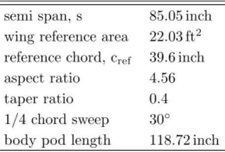
The reference geometry selected for HiLiftPW-1 is the NASA trapezoidal wing model. It is a large chord, semi-span, three element high lift wing configuration with a body pod. The body pod is mounted on a standoff, which is connected to a peniche on the tunnel wall. The half model wing has a semi-span of 85.1 inch and a comparatively low aspect ratio of 4.56. The wing is untwisted and has no dihedral. The taper ration is 0.4. For the first HiLiftPW only the full-span flap configuration is considered, featuring a single-slotted flap mounted on four flap brackets and sealed to the side of body, extending from wing root to wingtip. The flap chord ratio is 0.3, which is held constant across the span. At the leading edge, a constant chord, full-span slat is mounted on six slat brackets and also sealed to the side-of-body. The main dimensions of the model are listed in table 1, the settings of the high lift elements for the reference configuration are listed in table 2. Further details about the model are given by Slotnick et al.8
Table 1. Main dimensions of the trapezoidal wing model.
semi span, s 85.05 inch wing reference area 22.03 ft2
reference chord, cref 39.6 inch
aspect ratio 4.56 taper ratio 0.4 1/4 chord sweep 30◦ body pod length 118.72 inch
The model was tested in NASA Langley’s 14x22 and Ames’ 12 foot wind tunnels. For the present validation study only data of the 14x22 wind tunnel are considered. A description of the validation experiment is given by Johnson et al.9 Figure 1 shows the model installed in the 14x22 wind tunnel.
Table 2. Specification of the trapezoidal wing model in configuration 1.
slat deflection angle 30◦ slat gap, gs/cref 0.015
slat height, hs/cref 0.015
flap deflection angle 25◦ flap gap, gf/cref 0.015
flap overlap, of/cref 0.0026
(a) View from above; photo ID EL-1998-00248. (b) View from below.
Figure 1. NASA trapezoidal wing installed at Langley Research Center 14x22ft wind tunnel; photo courtesy of NASA.
III.
Test Cases
Participation to the workshop requires to deliver results for two cases (case 1 and case 2). The additional test case (case 3) is used to study the effects of the flap and slat supports.10 Two configurations of the
available trapezoidal wing lineup are used for HiLiftPW-1, configuration 1 and configuration 8, which differ in the deflection angle of the flap, see figure 2(a). To simplify the mesh generation, both baseline configurations do not include the flap and slat support brackets. Only the geometry of case 3 features the brackets, see figure 2(b) for a comparison of configuration 1 with and without brackets. A short description of each case along with the boundary conditions is given below.
(a) Different flap deflection angle for config-uration 1 and configconfig-uration 8.
(b) Configuration 1 with brackets (above) and clean, without brackets (below)
III.A. Case 1
Case 1 refers to the grid convergence study with at least three grid levels, to be performed for two angles of attack. The geometry features a deflection angle of the flap of 25◦ and a slat deflection angle of 30◦. The trapezoidal wing model with these settings for flap and slat is denominated configuration 1. The boundary conditions for this case are
• Mach number = 0.2,
• angle of attack = 13◦, 28◦,
• Reynolds number = 4.3·106.
III.B. Case 2
An additional configuration is used for case 2 to assess the effect of flap deflection over a range of angles of attack. Configuration 8 features a smaller flap deflection angle of 20◦. A computational grid is required for this configuration, comparable in size and resolution to the medium grid level of case 1. The boundary conditions are
• Mach number = 0.2,
• angle of attack = 6◦, 13◦, 21◦, 28◦, 32◦, 34◦ and 37◦,
• Reynolds number = 4.3·106.
III.C. Case 3
For the optional case 3, the supporting brackets of flap and slat are additionally modeled on configuration 1. The same conditions as for case 1 and a similar grid density allow for a comparison of the installation effects. The boundary conditions are
• Mach number = 0.2,
• angle of attack = 13◦, 28◦,
• Reynolds number = 4.3·106.
IV.
Computational Grids
The grid generation process remains the most influential factor in the overall accuracy of CFD tools. An appropriate physical model for the problem at hand is important to be able to capture the correct physical behavior. As a discrete problem is solved, the discretization has to be sufficient to harness the capabilities of a given physical model.11
To generate the grids for the Workshop, a similar approach is used, implemented in two different mesh generation packages, Centaur and Solar. The basic procedure is similar in that a surface mesh is first generated on the given surfaces, which is then extruded normal to the viscous wall surfaces into the volume. Subsequently the remaining field volume is filled by an advancing-front method with tetrahedra. Pyramidal elements are used to achieve a conforming interface between the near-field advancing-layer grid and the far-field advancing-front grid.
Centaur from CentaurSoft12 resolves surfaces with triangles, which leads to prismatic elements in the
near-wall regions. To reduce the number of surface elements, anisotropic triangular elements can be used, e.g. on the leading edge of the wing. Because of quality reasons the maximum anisotropic stretching is limited to values of about 2 to 10. During the past decade, extensive experience was gathered at DLR for the grid generation on complex aircraft configurations using Centaur with meshes up to 60 million points.
Solar discretizes the surfaces with a quad-dominant mesh, which allows for some triangles to improve the overall element quality. The amount of triangular surface elements is typically in the order of 0.3% of the total surface elements. Anisotropic quadrilateral elements enable to discretize simple-curvature surfaces, such as wing leading edges, in an optimal way. Due to the mixed-element surface grid, the advancing-layer step is hexahedra-dominant, with some triangle-based prismatic layer stacks. A quadrilateral surface grid
allows for elements with higher aspect ratios than triangles, while maintaining or even reducing discretization error for a given number of grid points. Solar has been developed jointly by ARA, QinetiQ, BAE Systems, and Airbus. Some of the recent algorithmic developments take place at ARA.13 Solar is mainly used in
the semi-automated mode, hereby the geometry of the configuration at hand is subdivided in several zones of either lifting surfaces or bodies. Afterwards a set of volume sources are automatically distributed for each component according to so-called philosophy files in which accumulated knowledge and best-practice guidelines are collected. For the purposes of the workshop contribution, the initial sources are then modified and manually complemented in certain regions of interest.
The two grid generation systems are under evaluation at DLR for several different application cases, with one of the most recent being the transonic NASA Common Research Model used for the fourth Drag Prediction Workshop.14
The prismatic-dominant grids generated with Centaur are available through the HiLiftPW-1 home page and are denominated “Unst-Mixed-Nodecentered-A-v1”. The hexahedra-dominant grids generated with Solar are denominated “Unst-Mixed-Nodecentered-B-v1”.
IV.A. Compliance to Grid Requirements
The workshop committee releases a set of guidelines to guarantee similar grid quality for all workshop contributions.7 In some points the guidelines discern between structured and unstructured grids. This
is necessary, as the generation of a family of truly self-similar unstructured grids is not possible with the standard advancing-layer/advancing-front approaches. Particular attention is paid to achieve a high level of self-similarity between the grid levels with both grid generation methods.
IV.A.1. Prismatic-dominant Grids
Most specifications are fulfilled by the Centaur meshes. The initial normal spacing as given in the gridding guidelines is used directly for the mesh generation. The prismatic layer stretching normal to the wall is a geometrical series in Centaur, therefore the requirement of having a minimum of two layers of constant spacing can not be met. The growth ratio normal to the viscous walls is kept below 1.25. The far-field distance is set to approx. 100·Cref, the discretization of the trailing edges follows also the guidelines.
IV.A.2. Hexahedra-dominant Grids
For the Solar grids, the meshing guidelines are fulfilled as far as the meshing package allows to. Some minor deviations from the gridding guidelines are summarized here.
Based on trial computations, to achievey+ values below unity on all viscous surfaces, the first cell height
is set considerably lower than the maximal allowed value given in the guidelines. The initial number of layers with constant spacing is scaled for each grid level to improve the similarity of the grid family. The target ratio of number of points between two grid levels is achieved with an accuracy of 1.5%. The recommended maximal value for the near-field growth rate of 1.25 is partially met. Due to the automatic, local growth rate modification, the coarse mesh features some regions of the main wing with a growth rate larger than 1.25. The capability to vary the growth rate is not implemented in Solar, so points e)2) and e)3) of the gridding guidelines7 can not be met. The requirement for a minimal resolution across the thick trailing edges of the
lifting surfaces is exceeded.
IV.B. Case 1
At least three solutions on a family of grids of varying size are required to perform Richardson extrapolation. The complete grid family has to lie within the asymptotic grid convergence range, this implies that all relevant aerodynamic phenomena have to be resolved on all three levels. For the three required grids (coarse, medium and fine) the committee guidelines call for a ratio of three in total number of points between two grid levels. IV.B.1. Prismatic-dominant Grids
To achieve the required surface discretization for the different grids, a fully automatic and parametric source generator is used, which controls the element sizes on the surface and in the flow field. As input the source generator uses the rules for the element sizes from the gridding guidelines, as output a so-called source
file for the Centaur mesh generator is written, which describes the local elements sizes of the mesh on the surface and in the field. Special attention is paid to have a smooth transition between the different sources to improve the quality of the flow solution. Typically this automated procedure leads to more than 5000 sources for the slat, main wing, flap and body (with peniche). Using this technique a grid family is built with consistent topology, grid sizes and scaling factors.
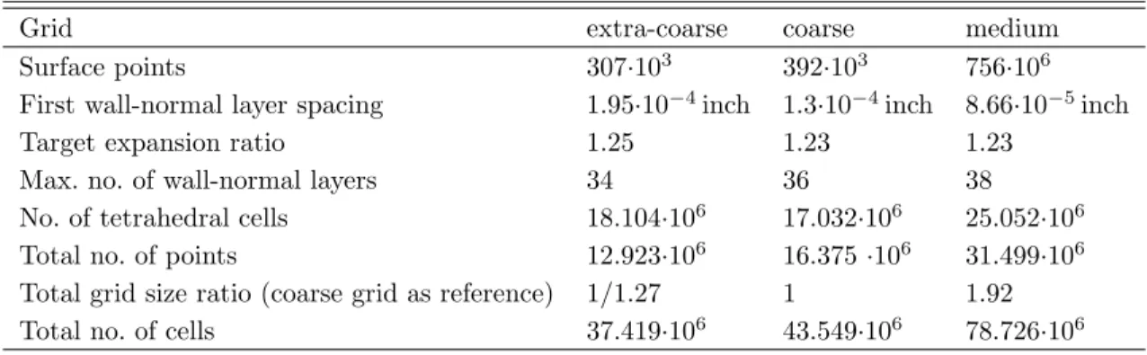
Based on the automatically generated sources, it is possible to build a coarse and medium mesh with Centaur. However, the fine (and extra fine) grid levels can not be built due to problems at the interface between the prisms and the tetrahedra. A fine grid level could only be obtained with significant deviations from the gridding guidelines, which in turn would destroy the grid family concept. Therefore it was decided to generate an extra-coarse grid level, instead of the fine one. The grid sizes and near-field grid generation parameters for the resulting three grids are summarized in table 3.
Table 3. Overall Centaur grids details and near-field parameters for case 1.
Grid extra-coarse coarse medium
Surface points 307·103 392·103 756·106
First wall-normal layer spacing 1.95·10−4inch 1.3·10−4inch 8.66·10−5inch
Target expansion ratio 1.25 1.23 1.23
Max. no. of wall-normal layers 34 36 38
No. of tetrahedral cells 18.104·106 17.032·106 25.052·106
Total no. of points 12.923·106 16.375·106 31.499·106
Total grid size ratio (coarse grid as reference) 1/1.27 1 1.92 Total no. of cells 37.419·106 43.549·106 78.726·106
IV.B.2. Hexahedra-dominant Grids
Since in Solar the target grid spacing is specified in distinct volume sources, a one-dimensional refine-ment/coarsening factor is required. A factor of three for a three-dimensional grid translates to a one-dimensional scaling factor of √33≈1.4422. Only this factor is used to scale the volumetric sources, whereas
the range of influence of the sources is not changed as it is linked to the geometry. A summary of the final grid family points and elements counts is given in table 4.
Table 4. Overall Solar grids details for case 1.
Grid coarse medium fine
Surface points 328·103 682·103 1.419·106
Max. no. of wall-normal layers 35 51 74
No. of points in prism/hexa layers 12.13·106 36.161·106 107.762·106
No. of tetrahedral cells 5.294·106 13.666·106 36.286·106
Total no. of points 12.307·106 36.968·106 110.746·106
Total grid size ratio (medium grid as reference) 1/2.9957 1 3.0038 Total no. of cells 16.785·106 48.5·106 141.308·106
The required input parameters for the near-field grid generation procedure are scaled with the same factor of √3
3. The values for the medium and fine levels are derived from the coarse grid, as the maximal target expansion ratio of 1.25 is used for the coarse grid. The relations between the grid levels in terms of first layer spacing and number of wall-normal layers should follow the scaling factor given above. Please notice that for the number of wall-normal layers, an integer value has to be used due to the nature of the advancing-layer process. Given the requirement for a self-similar total layer thickness, scaled first layer spacing and scaled total number of layers, leaves only the expansion ratio as variable to be determined for the medium and fine grids. The procedure is described in more detail by the author.11 The resulting input parameters for the
Table 5. Near-field Solar grids details.
Grid coarse medium fine
First wall-normal layer spacing 6·10−5inch 4.16017·10−5inch 2.8845·10−5inch
No. of cells with constant spacing 4 6 9
Expansion ratio [target; range] 1.25; 1.0123-1.3722 1.1664; 1.0009-1.2377 1.1122; 1.0002-1.1595
IV.C. Case 2
An additional grid for configuration 8 needs to be generated for case 2, similar in size and point distribution to the medium grid for configuration 1 of case 1. A grid for configuration 8 was only generated with Solar, not with Centaur. Since the only difference is constrained to the flap deflection angle, only the sources of the flap are transformed from configuration 1, the remaining background grid sources are the same for the two grids. The flap sources of configuration 1 are first transformed from deployed to stowed, then deployed with the parameters of configuration 8. Apart from the geometry and the flap sources, the grid generation settings are the same as for the medium grid of case 1. The details for the grid of configuration 8 are summarized in table 6. It is possible to recognize similar point counts and distribution to the medium grid for configuration 1 of case 1.
IV.D. Case 3
The configuration 1 with additional slat and flap support brackets is meshed only with Solar, not with Centaur. For a better comparison to the results for configuration 1 without brackets (case 1), the sources are not re-generated from scratch. Only the sources for the additional brackets are distributed and added to the available case 1 sources. The grid generation settings are the same as for the medium grid of case 1. The details for the grid of configuration 1 with brackets are summarized in table 6.
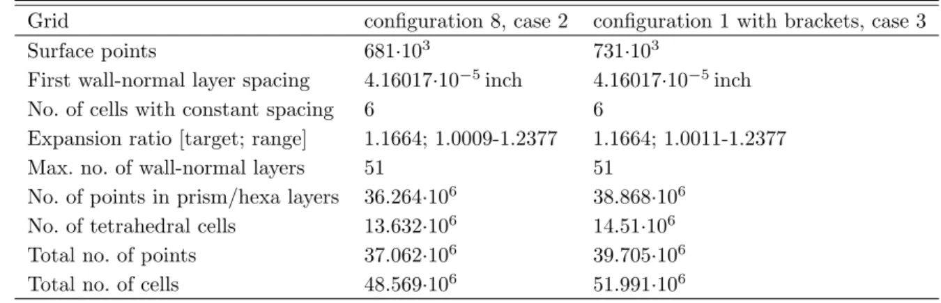
Table 6. Overall Solar grids details and near-field parameters for configuration 8 of case 2 and configuration 1 with brackets of case 3.
Grid configuration 8, case 2 configuration 1 with brackets, case 3 Surface points 681·103 731·103
First wall-normal layer spacing 4.16017·10−5inch 4.16017·10−5inch
No. of cells with constant spacing 6 6
Expansion ratio [target; range] 1.1664; 1.0009-1.2377 1.1664; 1.0011-1.2377 Max. no. of wall-normal layers 51 51
No. of points in prism/hexa layers 36.264·106 38.868·106
No. of tetrahedral cells 13.632·106 14.51·106
Total no. of points 37.062·106 39.705·106
Total no. of cells 48.569·106 51.991·106
IV.E. Other Grids
Selected computations are performed also on the full-hexahedra grids generated by Boeing, Huntington Beach with ANSYS ICEM CFD and made available by the workshop committee as the set “Unst-Hex-FromOnetoOne-A-v1”. For the remainder of this study, these grids are referred to simply as “1to1”. For the grid convergence study, the computations are performed on the extra-coarse, coarse and medium grids, with respectively 6.069, 20.357 and 48.105 million points.
IV.F. Corner Flow Discretization
The advancing-layer method may result in layer intersections in concave corners, if the initial wall-normal extrusion direction and extension are maintained. This is a common problem to all advancing-layer methods, that can be alleviated in several ways.
By default, in the vicinity of concave corners, Centaur decreases the first wall-normal spacing, modifies the wall-normal vector and may even constrain the amount of layers grown in the concave corners. An advanced setting used here is to also allow the growth ratio to be decreased to a minimum value of 1.1.
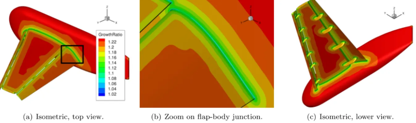
The typical approach used in Solar is to locally reduce the expansion ratio, so that the same amount of wall-normal layers are generated everywhere. The surface distribution of the advancing-layer expansion ratio is visualized exemplarily for the grid of case 3 in figure 3. The target for the expansion ratio for this
(a) Isometric, top view. (b) Zoom on flap-body junction. (c) Isometric, lower view.
Figure 3. Expansion ratio surface distribution for configuration 1 with brackets.
case is set to 1.1664 but the final values range from 1.0009 at the junction of slat trailing edge with the body to 1.2377 on parts of the body.
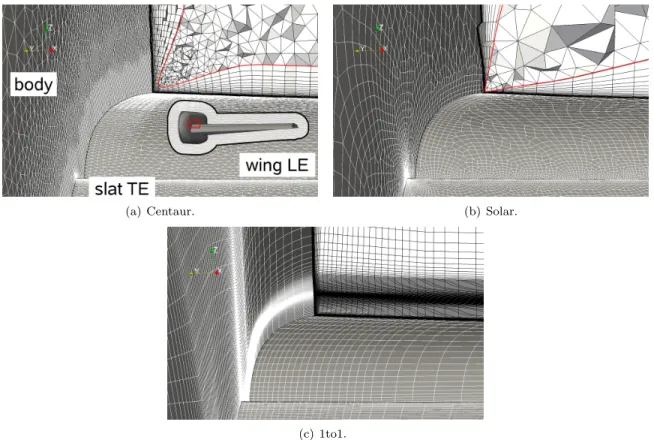
All measures taken by the advancing-layer grid generation algorithms lead to a local contraction of the prismatic/hexahedral layer. A comparison of the resulting corner discretization is given exemplarily at the nominal quarter-chord in figure 4. The approach used in Centaur leads to the layer contraction visible in figure 4(a). The strict wall-normal layer extrusion direction used in Solar can be recognized in figure 4(b). A decreasing expansion ratio towards the corner, leads to the depicted layer contraction. The isotropic tetrahedra elements that are inserted in the corner are not satisfactory, both in terms of element volume transition but also being obviously inappropriate to resolve the junction boundary layer. The tetrahedra in the corner of the Centaur grid are smaller and result in more benign volume transition. This is believed to be due to the base elements being isotropic triangles, which are better suited for the advancing-front tetrahedra generation step. In the Solar grid, the quadrilateral surface elements at the junction are anisotropic, i.e. stretched in the chord-wise direction. Although the stretching ratio is limited to 1:2, the resulting tetrahedra base elements of the final hexahedra layer, lead to larger tetrahedra than for the Centaur grid. It is also possible to recognize that the total extent of the near-field layer at the junction is bigger in the Centaur grid than in the Solar grid. An H-type corner discretization would be more appropriate, as is the case for the full-hexahedra 1to1 grid (fig. 4(c)), which features here a collar grid block. Such a topology allows not only to correctly resolve the corner flow, but also to capture the shear layer development of the upstream high-lift system element.
V.
TAU - Reynolds-averaged Navier-Stokes Solver
The Reynolds-averaged Navier-Stokes (RANS) solver TAU is under development at DLR. The roots of the software system date back to the consolidation project MEGAFLOW, which integrated developments of DLR, aircraft industry, and universities.15–17
The edge-based, finite volume, unstructured TAU solver uses the dual grid technique on hybrid grids. The employed numerical scheme is a spatially second-order accurate central scheme, using Jameson-Schmidt-Turkel artificial dissipation.18 Time integration is achieved either through an explicit Runge-Kutta multistage
scheme in combination with an explicit residual smoothing or a lower-upper symmetric Gauss-Seidel (LU-SGS) scheme. A geometric multi-grid method is available for convergence acceleration, using typically either 3V or 4W cycles.
Several turbulence models are available in TAU, three of which are used in the computations presented hereafter. The Spalart-Allmaras model19 (SA) is the standard model used in TAU. The one-equation eddy
viscosity model is particularly suited for external aeronautical aerodynamics with mainly attached flow regions. The Menter k-ω-SST model20is a two-equation eddy viscosity model, also developed specifically for
(a) Centaur. (b) Solar.
(c) 1to1.
Figure 4. Downstream view on surface grids of body, slat and wing (gray with white edges) and field cut (white with black edges) at nominal quarter chord; coarse grids.
aeronautical applications with a target to improve flow separation predictions. The SSG/LRR-ωdifferential Reynolds-stress model is the highest-fidelity physical model used for this study. Through the baseline ω -equation blending function from Menter, for supplying the length scale, a combination is achieved of the Launder-Reece-Rodi model near the walls and the Speziale-Sarkar-Gatski model further away.21
VI.
Results
The results presented hereafter are compared to experimental data gather in the last decade9, 22 and
provided to the participants by the workshop committee. For configuration 1, the surface pressure coefficient data at the nominal angles of attack of 13◦ and 28◦ is compared to the corrected experimental data from the NASA Langley 14x22ft wind tunnel test number 513, run 105 at 12.99◦ (point 274) and 28.41◦ (point 285), respectively. The forces and moments from the same test are used for configuration 1, whereas for configuration 8, the data from the NASA Langley 14x22ft wind tunnel test number 478, run 63 is used.
VI.A. Case 1
The focus of this case is on the assessment of grid-convergence for three grid families. A detailed presentation of the results is only given for the Solar and Centaur grids. The 1to1 grid family is only used to assess the global convergence of forces and moments.
VI.A.1. Forces and Moments Data
The grid-convergence for the integrated forces and pitch moment coefficient is plotted versus the grid index factor in figure 5 for the angle of attack (α) of 13◦ and in figure 6 forα= 28◦.
The grid index factor is the inverse of the total number of points to the power of 2/3 (N−2/3). The reason for plotting global values as a function of the chosen grid index factor is that a second-order convergence rate would show as a straight line. This is though only valid if the ratio of grid points between two consequent
N-2/3
C
L
0 1E-05 2E-05 3E-05 1.96 1.98 2 2.02 2.04 2.06 Solar Centaur 1to1
(a) Lift coefficient (CL)
N-2/3
C
D
0 1E-05 2E-05 3E-05 0.31
0.32 0.33 0.34 0.35
(b) Drag moment coefficient (CD)
N-2/3
C
M
0 1E-05 2E-05 3E-05 -0.5
-0.49 -0.48 -0.47 -0.46
(c) Pitch moment coefficient (CM) Figure 5. Grid convergence for Centaur, Solar and 1to1 grid families atα= 13◦.
grid levels is the same, i.e. if the ratio of coarse/medium is the same as medium/fine. A deviation from second-order convergence rate is found for all grids, but a similar ratio between two grid levels is only given for the 1to1 and Solar grids. Due to the grid generation difficulties encountered with Centaur, the ratios extra-coarse/coarse and coarse/medium are not comparable (see also table 3), introducing a further unknown in evaluating the results from the grid-convergence plots. Nonetheless it is possible to identify the grid-convergence trends for the three grid families.
At the lower angle of attack of 13◦, major differences are found between the grid families with respect to the convergence trend. In terms of absolute values, the range for all solutions on all grid levels is limited to 2 lift counts and 50 drag counts, see figures 5(a) and 5(b). The grid convergence for pitch moment coefficient (figure 5(c)) shows three different convergence trends for the three grid families.
N-2/3
C
L
0 1E-05 2E-05 3E-05 2.8 2.82 2.84 2.86 2.88 2.9 Solar Centaur 1to1
(a) Lift coefficient (CL)
N-2/3
C
D
0 1E-05 2E-05 3E-05 0.64
0.65 0.66 0.67 0.68
(b) Drag moment coefficient (CD)
N-2/3
C
M
0 1E-05 2E-05 3E-05 -0.44
-0.43 -0.42 -0.41
(c) Pitch moment coefficient (CM) Figure 6. Grid convergence for Centaur, Solar and 1to1 grid families atα= 28◦.
To allow for a relative comparison to the lower angle of attack, the data presented in figure 6 for an angle of attack of 28◦, is plotted with the same range of lift, drag and pitch moment coefficients, respectively 0.1, 0.04 and 0.04. Using the same range enables to perform a relative comparison between the two angles of attack. For all grid families, atα= 28◦ the spread of the results from coarsest to finest grid level is larger than atα= 13◦. The convergence trends of all force and moment coefficients are similar for all three grid families atα= 28◦.
The deviation of the fine-grid results from the coarse-medium trend of the Solar grid family, is more pronounced atα= 13◦than atα= 28◦. The Solar grid family shows also the least difference between coarse and fine grid values of all three grid families atα= 28◦, whereas it is comparable to the 1to1 grid family at
α= 13◦.
VI.A.2. Surface Pressure Data
The grid-convergence of a local quantity such as surface pressure coefficient can help to explain the global grid-convergence behavior. The following pressure coefficient plots are taken exemplarily at mid-chord (η=
50%) and at the wingtip (η = 98%), see figure 7 for the relative location of the surface cuts.
Figure 7. Location of pressure taps on main wing and flap atη= 50% andη= 98%.
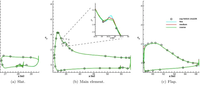
At mid-chord, the surface pressure coefficient can not be easily discerned between the three grid levels, both for the Solar (see figure 8 and 9) and Centaur results (data not shown). A grid-dependent suction peak is found atx≈35mon the main element. At this location, a surface curvature jump is present, where the slat trailing edge lies in stowed position. The different discretization of this geometrical discontinuity between the grid levels, leads to the only visible grid-dependent differences in surface pressure coefficient.
The pressure coefficient in several cut planes is basically grid-independent both atα= 13◦ and atα= 28◦ for the better part of the wing.
27 28 29 -10 -8 -6 -4 -2 0 cp x [m] exp NASA 14x22 fine medium coarse (a) Slat. 35 40 45 50 55 -8 -6 -4 -2 0 cp x [m] exp NASA 14x22ft fine medium coarse 33.5 34 34.5 35 35.5 36 -3.2 -3 -2.8 -2.6 cp x [m] exp NASA 14x fine medium coarse (b) Main element. 60 62 64 66 68 -6 -4 -2 0 cp x [m] exp NASA 14x22ft fine medium coarse (c) Flap. Figure 8. Surface pressure coefficient for computations on Solar grids atα= 13◦,η= 50%.
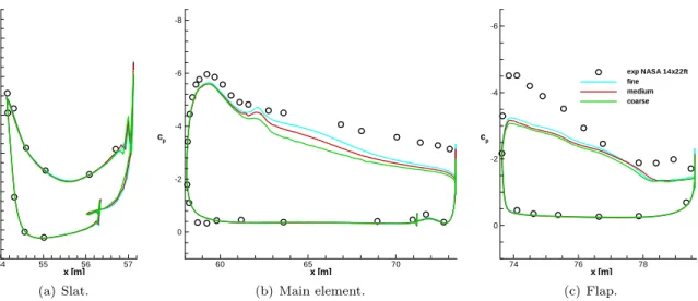
Only at the wingtip, a different convergence trend is found for the two angles of attack. At α= 13◦, the Solar results show that the pressure coefficient data on the fine grid deviates from the coarse-medium trend, see figure 10. No relevant grid-dependence is seen on the slat. On the main element, the fine-grid suction peak at the trailing edge lies between the values of the medium and coarse grids. The leading edge suction peak on the flap shows a similar deviation of the fine-grid result from the coarse-medium trend. The fine-grid peak is considerably lower than the peaks for the coarse and medium grids, which both better fit the experimental data. This is thought to be the reason for the deviation of the fine-grid solution from the coarse-medium trend in lift and pitch moment coefficient values presented in section VI.A.1.
At α= 28◦, the data at the wingtip shows a step-wise trend from coarse, medium to fine grid results, see figure 11. Although grid-independence is not achieved, the resulting forces and moments show a more consistent grid-convergence behavior than atα= 13◦.
27 28 29 -10 -8 -6 -4 -2 0 cp x [m] exp NASA 14x22 fine medium coarse (a) Slat. 35 40 45 50 5 -8 -6 -4 -2 0 cp x [m] exp NASA 14x22ft fine medium coarse (b) Main element. 60 62 64 66 68 -6 -4 -2 0 cp x [m] exp NASA 14x22ft fine medium coarse (c) Flap. Figure 9. Surface pressure coefficient for computations on Solar grids atα= 28◦,η= 50%.
54 55 56 57 -10 -8 -6 -4 -2 0 cp x [m] exp NASA 14x22 fine medium coarse (a) Slat. 60 65 70 -8 -6 -4 -2 0 cp x [m] exp NASA 14x22ft fine medium coarse 70 71 72 73 -5 -4.5 -4 -3.5 cp x [m] (b) Main element. 74 76 78 -6 -4 -2 0 cp x [m] exp NASA 14x22ft fine medium coarse (c) Flap. Figure 10. Surface pressure coefficient for computations on Solar grids atα= 13◦,η= 98%.
54 55 56 57 -10 -8 -6 -4 -2 0 cp x [m] exp NASA 14x22 fine medium coarse (a) Slat. 60 65 70 -8 -6 -4 -2 0 cp x [m] exp NASA 14x22ft fine medium coarse (b) Main element. 74 76 78 -6 -4 -2 0 cp x [m] exp NASA 14x22ft fine medium coarse (c) Flap. Figure 11. Surface pressure coefficient for computations on Solar grids atα= 28◦,η= 98%.
The Centaur results show a similar picture as the Solar results, both at α= 13◦ andα= 28◦. Atα= 13◦, the main element suction peak at the trailing edge shows a grid-dependent, but inconsistent behavior, in that the extra-coarse data lies between the coarse and medium grid data, see figure 12(b). An inconsistent grid-dependent behavior is also found on the flap, see figure 12(c).
54 55 56 57 -10 -8 -6 -4 -2 0 cp x [m] exp NASA 14x22 medium coarse extra-coarse (a) Slat. 60 65 70 -8 -6 -4 -2 0 cp x [m] exp NASA 14x22ft medium coarse extra-coarse 70 71 72 73 -5 -4.5 -4 -3.5 cp x [m] (b) Main element. 74 76 78 -6 -4 -2 0 cp x [m] exp NASA 14x22ft medium coarse extra-coarse (c) Flap. Figure 12. Surface pressure coefficient for computations on Centaur grids atα= 13◦,η= 98%.
Atα= 28◦, see figure 13, the results of the extra-coarse and coarse grids match relatively well, whereas the medium-grid results show a slight improvement on the main elements. The extra-coarse and coarse grids are relatively similar in the wingtip region, leading to similar results here.
54 55 56 57 -10 -8 -6 -4 -2 0 cp x [m] exp NASA 14x22 medium coarse extra-coarse (a) Slat. 60 65 70 -8 -6 -4 -2 0 cp x [m] exp NASA 14x22ft medium coarse extra-coarse (b) Main element. 74 76 78 -6 -4 -2 0 cp x [m] exp NASA 14x22ft medium coarse extra-coarse (c) Flap. Figure 13. Surface pressure coefficient for computations on Centaur grids atα= 28◦,η= 98%.
VI.A.3. Flow Topology
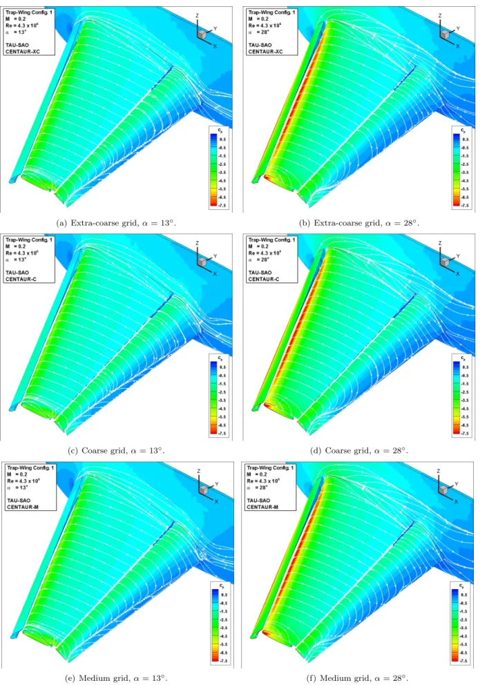
A macroscopic view on the near-wall flow field shows no major differences between the grid levels of the Solar and Centaur grid families. The surface pressure along with skin-friction lines on the three wing elements is presented in figure 14 for the Centaur grid family. From this macroscopic view, it is not possible to discern a difference in flap trailing edge separation between the three grid levels, both atα= 13◦andα= 28◦. A grid-dependent surface flow topology is visible at the flap-body junction, but only at α= 13◦, see figures 14(a), 14(c) and 14(e).
(a) Extra-coarse grid,α= 13◦. (b) Extra-coarse grid,α= 28◦.
(c) Coarse grid,α= 13◦. (d) Coarse grid,α= 28◦.
(e) Medium grid,α= 13◦. (f) Medium grid,α= 28◦.
Atα= 13◦ the results on the Solar grids show a similar surface flow topology as on the Centaur grids, see figure 15. On the coarse grid, the flow on the flap is seemingly fully attached, but an off-body separation
(a) Coarse grid. (b) Medium grid.
(c) Fine grid.
Figure 15. Surface skin friction lines at flap-body junction for computations on Solar grids atα=13◦.
produces a focus-type critical point on the body. On the medium grid, the body focus-type critical point remains, but an additional focus point appears on the flap trailing edge. The separation on the flap increases considerably in size on the fine grid. This has an impact also on the skin-friction pattern of the body, which shows signs of reversed flow coming from below the flap. In terms of flap-body junction flow, grid-independence is thus not achieved neither for the Centaur nor for the Solar grid family atα= 13◦.
Atα= 28◦the flap-body junction is also present, but the topology and separation size show only a minor
grid-dependence, both in the Centaur grid results (see figures 14(b), 14(d) and 14(f)) and in the Solar grid results (data not shown).
The different grid-dependent behavior at the flap-body junction is believed to be one of the reasons why the global grid-convergence trends presented in section VI.A.1 are more consistent atα= 28◦ than at α= 13◦.
VI.B. Case 2
The angle-of-attack sweep is performed for both configurations only using the Solar medium grids, whereas only the Centaur medium grid of case 1 is used for the sweep of case 2. The lift, drag and pitch moment coefficients are shown in figure 16 for configuration 1 and figure 17 for configuration 8.
α C L 5 10 15 20 25 30 35 1.5 2 2.5 3 exp NASA 14x22ft case2; conf1 case3; conf1 w/brackets
(a) Lift coefficient (C-lift)
α C D 5 10 15 20 25 30 35 0.2 0.4 0.6 0.8
(b) Drag coefficient (C-drag)
α C M 5 10 15 20 25 30 35 -0.5 -0.4 -0.3 -0.2
(c) Pitch moment coefficient (C-my) Figure 16. Angle of attack sweep for Solar grids; case2 and case3, configuration 1.
α C L 10 20 30 1.5 2 2.5 3 exp NASA 14x22ft case2; conf8
(a) Lift coefficient (C-lift)
α C D 5 10 15 20 25 30 35 0.2 0.4 0.6 0.8
(b) Drag coefficient (C-drag)
α C M 5 10 15 20 25 30 35 -0.5 -0.4 -0.3 -0.2
(c) Pitch moment coefficient (C-my) Figure 17. Angle of attack sweep for Solar grids; case2, configuration 8.
The higher flap deflection angle of configuration 1 leads to higher lift and drag as well as smaller pitch moment over the entire angle of attack range. The computations match relatively well the slope and absolute values of lift and drag, but are slightly offset for the pitch moment. Due to the smaller flap deflection angle of configuration 8, the same angle of attack range does not end into the fully-separated post-stall region as with configuration 1.
With the Centaur grid, the results on configuration 1 (see figure 18) are similar to the Solar results for angles of attack below 30◦.
α C L 5 10 15 20 25 30 35 1.5 2 2.5 3 exp NASA 14x22ft case2; conf1
(a) Lift coefficient (CL)
α C D 5 10 15 20 25 30 35 0.2 0.4 0.6 0.8 (b) Drag coefficient (CD). α C M 5 10 15 20 25 30 35 -0.5 -0.4 -0.3 -0.2
(c) Pitch moment coefficient (CM) Figure 18. Angle of attack sweep for Centaur grids; case2, configuration 1.
Near to the maximal lift coefficient, the Centaur results lie above the experimental data, whereas the Solar results lie below. The difference between Solar and Centaur results in terms of drag coefficient are not as large as for lift and pitch moment coefficient. The pitch moment coefficient values for Centaur are closer to the experimental data below 20◦. Above 20◦, the Solar results are closer to the experimental data.
VI.C. Case 3
The addition of slat and flap brackets to the discretized configuration 1, should result in better agreement to the experimental data. The wind-tunnel model obviously features the brackets for holding the slat and flap. The brackets have an influence on the flow-field, as they disrupt the span-wise flow from the body to the tip in the slat and main element coves. Furthermore, the disturbed boundary layer on the lower side of the main element should have a detrimental effect on the flap, resulting in lower lift contribution from this element. Only two angles of attack are computed for case 3,α= 13◦andα= 28◦. The forces and moments
are plotted in figure 16 of the previous section for a better comparison to the clean configuration 1. Atα= 13◦, the brackets have only a minor effect on all coefficients, but atα= 28◦the lift coefficient decreases by 8 lift counts. As mentioned above, this is not expected as the addition of the brackets should result in a better match to the experimental data. The only explanation for this is that an aerodynamic phenomenon is not captured on neither grid, independently of the brackets. An under-resolved wingtip vortex system might be the main contributing factor.
The surface pressure coefficient plots at α= 13◦ confirm the relative small effect of the brackets, both atη = 50% (figure 19(a)) andη = 98% (figure 19(b)).
60 62 64 66 68 -6 -4 -2 0 cp x [m] exp NASA 14x22ft case1; conf1 case3; conf1 w/brackets
(a) Flap,η= 50%. 74 76 78 -6 -4 -2 0 cp x [m] exp NASA 14x22ft case1; conf1 case3; conf1 w/brackets
(b) Flap,η= 98%.
Figure 19. Surface pressure coefficient for computations on Solar grids atα= 13◦; brackets installation effects, case 1 without brackets (solid curve), case 3 with brackets (dashed curve).
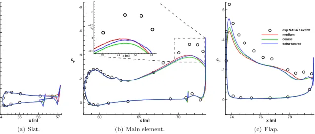
At the angle of attack of 28◦, the mid-span section shows the expected improvement towards the
exper-imental data by adding the brackets, see figure 20(a). The configuration without brackets predicts a larger lift on the flap. At the wingtip, at the same angle of attack, the results with or without brackets are similar, see figure 20(b). A considerable deviation from the experimental pressure coefficient on the flap tip, does not only lead to lower lift, but also to a larger pitch moment coefficient as seen in figure 16(c).
VI.D. Convergence Behavior
Usually the field is initialized with the free-stream values and thus convergence is from “scratch” towards the steady-state solution. For some conditions, this procedure leads to a stable steady-state solution that deviates substantially from the experimental data. The existence of more than one steady flow condition for high-lift airfoils is known from experimental studies,23, 24but also from numerical studies on a fully turbulent
NACA 0012 airfoil.25 Dual solutions are mostly found around maximum lift, but an influence of the initial
60 62 64 66 68 -6 -4 -2 0 cp x [m] exp NASA 14x22ft case1; conf1 case3; conf1 w/brackets
(a) Flap,η= 50%. 74 76 78 -6 -4 -2 0 cp x [m] exp NASA 14x22ft case1; conf1 case3; conf1 w/brackets
(b) Flap,η= 98%.
Figure 20. Surface pressure coefficient for computations on Solar grids atα= 28◦; brackets installation effects, case 1 without brackets (solid curve), case 3 with brackets (dashed curve).
previous solution, i.e. at the lower angle of attack of 13◦, leads to the same result as an initialization from free-stream values. Only a stepwise increase of angle-of-attack leads to the final values as presented above. The numerical convergence for case 1 atα= 28◦ is shown in figure 21 for the Centaur medium grid.
(a) From scratch. (b) Restart from solution atα= 13◦with intermediate
∆αsteps.
Figure 21. Solver convergence for computations on Centaur medium grid atα= 28◦.
Initializing the field with the free-stream values leads to a value of lift coefficient around 2.05, with the normalized density residual at approx. 2·10−6(figure 21(a)). A second approach is to start from the converged
α= 13◦ field solution and increase the angle of attack in several steps of approx. 2◦, see figure 21(b). The final lift coefficient for this case is 2.896, considerably higher and nearer to the experimental data than the lift coefficient for the computation from scratch at 2.05.
A comparison of the final lift coefficient values for this case is shown in figure 22(a). A similar influence on the initial condition is also found for the Solar grids, although only for the case 2, configuration 8 medium grid, see figure 22(b).
α C L 5 10 15 20 25 30 35 1.5 2 2.5 3 exp NASA 14x22ft αincrease scratch
(a) Centaur, medium grid configuration 1.
α C L 10 20 30 1.5 2 2.5 3 exp NASA 14x22ft αincrease scratch
(b) Solar grid, configuration 8.
Figure 22. Comparison of lift coefficient between computations started from scratch or from previous angle of attack with intermediate∆αsteps (αincrease).
VI.E. Turbulence Model Influence
A turbulence model variation was carried out limited to the medium Centaur grid. For this purpose the baseline SA model is compared to the two-equation k-ω SST model of Menter, and DLR’s differential Reynolds stress model (SSG/LLR-ω), designated as RSM. In general, only minor differences are detected for the three different turbulence models, although the level of sophistication is considerably increased. As an example the pressure distributions on the three elements at an angle of attack of 28◦are shown in figure 23 at a span-wise station of η = 50%. For the slat and the wing a good agreement between the wind tunnel
27 28 29 -10 -8 -6 -4 -2 0 cp x [m] exp NASA 14x22 SA SST RSM (a) Slat. 35 40 45 50 55 -8 -6 -4 -2 0 cp x [m] exp NASA 14x22ft SA SST RSM (b) Main element. 60 62 64 66 68 -6 -4 -2 0 cp x [m] exp NASA 14x22ft SA SST RSM (c) Flap
Figure 23. Surface pressure coefficient for computations on Centaur grid atα= 28◦; turbulence model comparison for
η= 50%.
data and the CFD results is obtained. A deviation between measured and computed results is seen on the flap upper side, where all turbulence models over-predict the suction level in the front part of the flap, and under-predict the separation tendency towards the trailing edge. As demonstrated in section VI.C, this deviation is mainly caused by neglecting the slat and flap brackets. As this is a geometrical effect, and not due to physical modeling, the results of the turbulence model variation appear to be consistent.
Larger differences between the turbulence model approaches can be found in the corresponding pressure distributions close to the wingtip at η = 98% in figure 24. The results of the SA model are characterized by a fair agreement to the experimental pressure distributions for the flap and the main wing. The suction level towards the wing trailing edge is under-predicted, and consistently also the suction peak on the flap is significantly too low in the computational results. In contrast to this, the results of the SST and the RSM
54 55 56 57 -10 -8 -6 -4 -2 0 cp x [m] exp NASA 14x22 SA SST RSM (a) Slat. 60 65 70 -8 -6 -4 -2 0 cp x [m] exp NASA 14x22ft SA SST RSM (b) Main element. 74 76 78 -6 -4 -2 0 cp x [m] exp NASA 14x22ft SA SST RSM (c) Flap
Figure 24. Surface pressure coefficient for computations on Centaur grid atα= 28◦; turbulence model comparison for
η= 98%.
models exhibit strong deviations to the experimental pressures on all three elements. On the main wing both SST and RSM indicate widely separated flow from about 30% wing chord towards the trailing edge. Also the suction levels on the flap surface are strongly under-predicted by both models with RSM showing the largest deviations and the highest pressure levels. The analysis of the turbulence model data implies, that the SA model yields a superior agreement to the experimental evidence. Yet, it requires further studies to confirm this conclusion. The general deviations of all three models at the rear part of the main wing and the flap may be linked to shortcomings in the computation of the slat edge vortex and its induced velocities on the rear part of the wingtip, due to e.g. insufficient grid resolution. A local grid refinement study is required to finally assess the simulation quality of the considered modeling approaches.
For the lower angle of attack of 13◦, velocity difference plots in the flow-field between the SA and the SST models (figure 25(a)), and the SA model and RSM (figure 25(b)) reveal the areas of the largest differences between the solutions. All models show significant differences close to the wingtip. Moreover, the SST model
(a) SA−SST. (b) SA−RSM.
Figure 25. Turbulence model comparison through velocity difference for computations on Centaur grid atα= 13◦.
exhibits differences to the SA model with respect to the side of body separation for this angle of attack. The lift curve in figure 26 proves the lower lift coefficients of the SST and the RSM model for both considered angles of attack. The difference between both SST and RSM results to the SA result is of similar magnitude at both angles of attack. The reason for the deviation of the SST and RSM results is present at both angles of attack, independently of the wing loading, which further strengthens the hypothesis of an under-resolved wingtip vortex system.
α C L 5 10 15 20 25 30 35 1.5 2 2.5 3 exp NASA 14x22ft SA SST RSM
Figure 26. Comparison of lift coefficient between computations on Centaur medium grid for different turbulence models (SA, SST, RSM).
VII.
Conclusions
The DLR contribution to the first AIAA High Lift Prediction Workshop is summarized in this paper. Hybrid computational grids for two configurations of the NASA trapezoidal wing are generated with the grid generation packages Centaur and Solar. For specific conditions, a workshop-provided full-hexahedra grid was also employed. Computations were performed with the DLR TAU code for all three defined cases and evaluated mainly with respect to lift, drag and pitch moment coefficients, as well as surface pressure coefficient at selected locations. In addition to the standard TAU turbulence model, the one-equation Spalart-Allmaras model, some computations are performed with the Menter k-ω-SST model and a differential Reynolds stress model.
A grid generation process is used with Solar that was shown in previous studies to produce a nearly self-similar family of grids for a grid-convergence study. After the successful application of this process to the Common Research Model of the fourth Drag Prediction Workshop, this process is used for the first time on a high-lift configuration. In a similar effort for the other employed grid generation package, Centaur, a newly developed, semi-automatic source distribution tool is used here to improve the grid similarity between grid levels.
The grid convergence trends are more satisfactory for the higher angle of attack of α= 28◦ than forα
= 13◦, although the scatter of the resulting values is smaller for the lower angle of attack. The results of the grid-convergence study suggest that none of the grid families lies in the asymptotic grid convergence range. This is either due to minor differences in specific regions, such as the side-of-body separation at the flap-body junction, or to major under-resolved features such as the wingtip vortex system.
The results using Solar- or Centaur-generated grids are quite comparable up to maximum lift with respect to lift and drag coefficient. Larger differences are only found after maximum lift and at post-stall angles of attack. The pitch moment coefficient shows a higher dependency to the employed grid system throughout the angle of attack range.
From the analysis of the surface pressure data, both in terms of absolute values, but also through the pronounced grid-dependency, an insufficient discretization of the wingtip region is suspected. This assumption is further strengthened by analyzing the results of different turbulence models.
Furthermore, it was observed that at certain conditions, two fully stable steady-state numerical results can be achieved. Substantially different results can be obtained, either when initializing the computation with free-stream values (from “scratch”) or with a solution from a previous angle of attack and then increasing stepwise the angle of attack. Dual solutions can be obtained for both configurations well before stall.
References
1Lindblad, I. A. A. and de Cock, K. M. J., “CFD prediction of maximum lift of a 2D high lift configuration,” Paper 99-3180, AIAA, June 1999, Applied Aerodynamics Conference.
2Rudnik, R., Melber, S., Ronzheimer, A., and Brodersen, O., “Three-Dimensional Navier-Stokes Simulations for Transport Aircraft High Lift Configurations,”Journal of Aircraft, Vol. 38, No. 5, September-October 2001, pp. 895–903.
3Thiede, P., “EUROLIFT – Advanced High Lift Aerodynamics for Transport Aircraft,”Air & Space Europe, Vol. 3, No. 3/4, May-August 2001, pp. 105–108.
4Rudnik, R. and Thiede, P., “European Research on High Lift Aircraft Configurations in the EUROLIFT Projects,”
Conference proceedings of the CEAS/KATnet Conference on Key Aerodynamic Technologies, 2005, pp. 16.1–16.8.
5Rudnik, R. and Germain, E., “Reynolds-Number Scaling Effects on the EUROPEAN High Lift Configurations,”Journal
of Aircraft, Vol. 46, No. 4, July-August 2009, pp. 1140–1151.
6Rudnik, R., Eliasson, P., and Perraud, J., “Evaluation of CFD methods for transport aircraft high lift systems,”The
Aeronautical Journal, Vol. 109, No. 1092, February 2005, pp. 53–64.
7High Lift Prediction Workshop committee, “1st AIAA CFD High Lift Prediction Workshop Gridding Guidelines,”http: //hiliftpw.larc.nasa.gov/Workshop1/GriddingGuidelinesHiLiftPW1-11JUN09.pdf, June 2009, Retrieved December 2010.
8Slotnick, J. P., Hannon, J. A., and Chaffin, M., “Overview of the 1st AIAA CFD High Lift Prediction Workshop,” Paper 2011-0862, AIAA, Orlando, FL, January 2011.
9Johnson, P. L., Jones, K. M., and Madson, M. D., “Experimental investigation of a simplified 3D high lift configuration in support of CFD validation,” Paper 2000-4217, AIAA, Denver, CO, August 2000, Applied Aerodynamics Conference and Exhibit.
10High Lift Prediction Workshop committee, “Test cases & data, 1st AIAA CFD High Lift Prediction Workshop,”http: //hiliftpw.larc.nasa.gov/Workshop1/testcases.html, 2009, Retrieved December 2010.
11Crippa, S., “Application of Novel Hybrid Mesh Generation Methodologies for Improved Unstructured CFD Simulations.” Paper 2010-4672, AIAA, June 2010.
12Kallinderis, Y., “Hybrid Grids and Their Applications.”Handbook of Grid Generation, edited by J. F. Thompson, B. K. Soni, and N. P. Weatherill, chap. 25, CRC Press, 1999.
13Leatham, M., Stokes, S., Shaw, J. A., Cooper, J., Appa, J., and Blaylock, T., “Automatic Mesh Generation for Rapid-Response Navier-Stokes Calculations,”FLUIDS 2000 Conference and Exhibit, June 2000, AIAA 2000-2247.
14Brodersen, O., Crippa, S., Eisfeld, B., Keye, S., and Geisbauer, S., “DLR Results from the Fourth AIAA CFD Drag Prediction Workshop,”28th AIAA Applied Aerodynamics Conference, June 2010, AIAA 2010-4223.
15Gerhold, T., Galle, M., Friedrich, O., and Evans, J., “Calculation of Complex Three-Dimensional Configurations Em-ploying the DLR-Tau Code,” Paper 97-0167, AIAA, 1997.
16Kroll, N., Rossow, C.-C., Becker, K., and Thiele, F., “MEGAFLOW - A Numerical Flow Simulation System,”Aerospace
Science Technology, 2000, pp. 223–237.
17Schwamborn, D., Gerhold, T., and Heinrich, R., “The DLR TAU-Code: Recent Applications in Research and Industry,”
In Proceedings of the European Conference on Computational Fluid Dynamics, ECCOMAS CFD 2006, edited by P. Wesseling, E. O˜nate, and J. P´eriaux, The Netherlands, 2006.
18Jameson, A., Schmidt, W., and Turkel, E., “Numerical Solution of the Euler Equations by Finite Volume Methods using Runge-Kutta Time Stepping Schemes,” Paper 81-1259, AIAA, Jan. 1981.
19Spalart, P. R. and Allmaras, S. R., “A One-Equation Turbulence Model for Aerodynamic Flows,” La Recherche
A´erospatiale, Vol. 1, 1994, pp. 5–21.
20Menter, F. R., “Two-Equation Eddy-Viscosity Turbulence Models for Engineering Applications,”AIAA Journal, Vol. 32, 1994, pp. 269–289.
21Eisfeld, B., “Numerical Simulation of Aerodynamic Problems with the SSG/LRR-ωReynolds Stress Turbulence Model Using the Unstructured TAU Code,”New Results in Numerical and Experimental Fluid Mechanics VI, Vol. 96 ofNotes on Numerical Fluid Mechanics and Multidisciplinary Design, Springer-Verlag, 2007, pp. 356–363, 15. DGLR/STAB-Symposium.
22Watson, R. D., Jenkins, L. N., Yao, C.-S., McGinley, C. B., Paschal, K. B., and Neuhart, D. H., “PIV Measurements in the 14 x 22 Low Speed Tunnel: Recommendations for Future Testing,” Techn. Mem. NASA/TM-2003-212434, NASA Langley Research Center, August 2003.
23Biber, K. and Zumwalt, G. W., “Hysteresis Effects on Wind Tunnel Measurements of a Two-Element Airfoil,” AIAA
Journal, Vol. 31, No. 2, 1993, pp. 326–330.
24Landman, D. and Britcher, C. P., “Experimental Investigation of Multielement Airfoil Lift Hysteresis due to Flap Rig-ging,”AIAA Journal of Aircraft, Vol. 38, No. 4, 2001, pp. 703 – 708.
25Mittal, S. and Saxena, P., “Hysteresis in flow past a NACA 0012 airfoil,”Computer Methods in Applied Mechanics and