The Balassa-Samuelson model in general equilibrium with markup variations

The Balassa-Samuelson model in general equilibrium

with markup variations

Université Université de Paris Ouest Nanterre La Défense

(bâtiments K et G)

200, Avenue de la République

92001 NANTERRE CEDEX

Tél et Fax : 33.(0)1.40.97.59.07

Document de Travail

Working Paper

2009-39

Romain Restout

E

c

o

n

o

m

iX

http://economix.u-paris10.fr/

The Balassa-Samuelson model in general

equilibrium with markup variations

Romain RESTOUT

Abstract

This contribution embeds the Balassa-Samuelson hypothesis in a general equilib-rium model that combines monopolistic competition and markup variations to examine the determinants of relative prices of nontradables. The model emphasizes the role of markup variations as an important aspect driving relative price movements. Variations in the markup makes fiscal policy non-neutral and provides a strong magnification mechanism for shocks to productivity. The empirical evidence of these predictions are examined by using a panel cointegration framework. On the whole, the econometric findings support theoretical implications, suggesting that our model is more closely in line with data relative to the supply-side Balassa-Samuelson framework that abstracts from variations in the degree of competition.

Keywords: Balassa-Samuelson effect, Monopolistic competition, Fiscal policy.

J.E.L. Classification: E20, E62, F31, F41.

1_{Romain RESTOUT, University Paris Ouest-Nanterre La D´efense (EconomiX) and Ecole Normale} Sup´erieure LSH (Gate). Address: Universit´e Paris Ouest-Nanterre La D´efense, 200 avenue de la R´epublique, 92001 Nanterre Cedex, France. Phone: +33 (0)1 40 97 59 63. Fax: +33 (0)1 40 97 59 07. E-mail address: [email protected]. I am indebted to Sophie B´ereau, Olivier Cardi, Nelly Exbrayat, Val´erie Mignon and Alain Sand for valuable comments. The usual disclaimers apply.

1

Introduction

More than forty-five years ago, Balassa [1964] and Samuelson [1964] developed an elegant and tractable model for addressing international prices discrepancies in a static environment characterized by perfect competition and frictionless markets. Their key insight is to identify variations in total factor productivity differentials between traded and non traded goods sectors to be the only exogenous driving force for relative prices. That interpretation has an important corollary: being determined independently of optimal intertemporal decisions by households and the government, the equilibrium path of the relative price requires only a description of the supply-side of the economy. Hence, the model embraces the dichotomy between supply and demand sides of the economy and accepts the complete irrelevance of fiscal policy with respect to relative prices. This result arises since the model assumes neoclassical hypotheses: an exogenous interest rate, perfect competition, the law of one price for tradable goods, constant returns to scale, and perfect mobility of factors across sectors. Both its reliance on technological disturbances as the primary source of relative prices fluctuations and its reliance on the strong assumptions above are, however, potential weak-nesses encountered by the Balassa-Samuelson model. That belief is underpinned by a large body of theoretical work which aims to reformulate the intuitive arguments of the Balassa-Samuelson theory within a micro-founded intertemporal framework featuring market failures or nominal rigidities. Early examples are Rogoff [1992] and De Gregorio et al. [1994a] who emphasize that imperfect factors mobility across sectors and wage rigidities may generate effects of fiscal shocks on the relative price. A more recent strand of the international macroeconomic literature allows for an endogenous Balassa-Samuelson effect by assuming firms entry (Ghironi and Melitz [2005]), endogenous tradability (Bergin et al. [2006]) or spatial distribution of firms (M´ejean [2008]). In addition to these inefficiencies, the present model combines monopolistic competition and markup variations, as a means for generating departures from the Balassa-Samuelson hypothesis. This framework allows us to investi-gate, both theoretically and empirically, the general equilibrium link between the relative price and exogenous shocks to productivity and government spending in a framework that encompasses variation in the degree of competition.

On the theoretical side, the contribution of the paper is to embed the static Balassa-Samuelson hypothesis in an explicitly dynamic general equilibrium model where variations in the composition of demand for nontradables give rise to endogenous changes in the markup. Within the non traded goods sector, preferences are such that the price elasticity of demand faced by the typical firm and consequently its markup are related to the relative weight of government spending in demand for nontradables. In this model, the relative price level results therefore from the general equilibrium outcome of the economy. As a result, any shock to agents’ environments which generates an endogenous markup variations gives rise to changes in the relative price. Thus, variation in the degree of competition provides a channel through which the direct impact of macroeconomic shocks is transmitted.

The model carries two theoretical implications for the relative price of non traded goods. The first finding is that positive fiscal shocks lead to persistent relative price appreciations. Within this framework, all the effects of government expenditure changes are channelled

through markup variations, the key new driving force in the model. With composition effects, an increase in domestic government spending enlarges the importance of the price-inelastic component of demand causing a fall in the price elasticity. This provides an in-centive for monopolistic producers to increase markups and prices. In this way, the model matches the evidence stemming from the recent empirical research.1 _{The second implication}

indicates that the variation in the markup provides a powerful magnification mechanism for shocks to productivity. Specifically, the default to account for the markup response to tech-nological shocks leads to understate their true effects. Indeed, we show that monopolistic firms respond to productivity shocks in either tradables or nontradables sector by modify-ing markups. This effect feedbacks in turn to the relative price and exacerbates the direct impact of the shocks. Based on the quantitative properties of the framework, it is estimated that around 28% of the variation in the relative price induced by a technology shock in the non traded goods sector can be attributed to the endogenous markup variation mechanism. The empirical part of the paper uses data for a panel of thirteen OECD economies over 1970-2004 to investigate the model’s theoretical implications. Before presenting the results in more detail, it is worth emphasizing that the model provides one refinement to augment the standard empirical estimates of the Balassa-Samuelson hypothesis. A potential concern with these estimates is that Solow residuals, used commonly to measure total factor productivity gains (TFP for short), contain measurement error owing to the presence of monopoly power.2

This drawback motivates our alternative measure which accounts for that nuisance element. We first test the predictions of the Balassa-Samuelson framework using Solow residuals for purposes of comparability. Although the model correctly predicts the direction of the effects of sectoral TFPs on the relative price, it does not correctly predict the magnitude because of measurement errors. When using our relevant productivity proxy, coefficient estimates on sectoral productivity fall dramatically, suggesting that previous standard Balassa-Samuelson estimates have been misspecified.

The second part of the empirical investigation tests model’s predictions by including proxies for product market competition and fiscal policy as additional explanatory vari-ables. These two factors are found to be significant and robust determinants of relative prices, in accordance with the theoretical results above. In particular, our findings uncover that expansive fiscal policies tend to fuel nontradables inflation, while deregulation policies may provide disinflation gains. Moreover, controlling for product market competition lowers significantly the estimated effects of productivity in nontradables, in a manner consistent with model’s predictions. This result explains why less competitive economies may experi-ence higher inflation since transmission mechanisms of productivity gains in nontradables into relative price reductions are eroded by increases in markups.

The remainder of the paper is structured as follows. Section 2 introduces the benchmark two-sector model. Section 3 discusses transmission mechanisms of fiscal and technological shocks to the relative price of nontradables. In section 4, we conduct a numerical analysis. Section 5 presents our econometric results. The final section 6 concludes.

1_{See Froot and Rogoff [1991], De Gregorio et al. ([1994a], [1994b]) and Balvers and Bergstrand [2002].} 2_{De Gregorio et al. [1994b], Kakkar [2003], Lee and Tang [2007] and MacDonald and Ricci [2007] 1992),} among others, have employed Solow residuals to measure productivity.

2

The framework

Consider a small open economy populated by a representative household, firms and a gov-ernment. There are two sectors in the economy producing an homogeneous traded good T and a differentiated non traded goodN. The traded good serves as the numeraire (pT _{= 1)}

and the law of one price prevails in that sector. The model features two distinct roles for non traded goods: as final consumption and as an input into the production of traded and non traded goods.3

2.1

Households and government

The representative household gains utility from its consumptioncand experiences disutility from supplying labor denoted byL. The felicity function is assumed to take the form

Z ∞ 0 _c1−1/σ 1−1/σ −γ L1+1/σL 1 + 1/σL e−βt_{dt, (1)}

where β ∈(0,1) denotes the consumer’s discount rate, σ > 0 the intertemporal elasticity of substitution, σL > 0 the Frisch elasticity of labor supply, and γ is a positive scaling

parameter of disutility of work. The composite consumption good is a CES aggregate of traded and non traded consumptions,cT _andcN _respectively

c=hϕ1/φ cT(φ−1)/φ

+ (1−ϕ)1/φ cN(φ−1)/φiφ/(φ

−1)

, (2) where ϕ∈(0,1) parameterizes the relative importance of traded and non traded goods in consumption, andφ >0 reflects the intratemporal elasticity of substitution. The preferences over the non traded goods are described by the familiar bundles of differentiated goods

cN = Z 1 0 cN(z)(θ−1)/θ_dz θ/(θ−1) , (3) withθ >1 is the symmetric elasticity of substitution across non traded goods.

The household decision problem is solved by the means of two-stage budgeting. In the first stage, the consumer chooses a time profile for consumption, labor supply and financial assetsa(t) to maximize the utility function (1) subject to her/his budget constraint:

˙

a(t) =r∗

a(t) + Π(t) +w(t)L(t)−πc(t)c(t)−Z(t), (4) wherer∗_{is the exogenous world interest rate, Π the profit income,wthe real wage,π}c _{is the}

consumption-based price index and Z denotes lump-sum taxes.4 _{Lettingλ be the shadow}

value of wealth, the first-order conditions characterizing the household’s optimal plans are uc = λπc, (5a)

uL = −λw, (5b)

˙

λ = λ(β−r∗

), (5c)

3_{Brock and Turnovsky [1994] develop a model in which capital goods are either traded or non traded.} They find that it is the relative sectoral intensity of nontradable capital that matters for model’s dynamics. 4_{In this setup, dots indicate time derivatives, while subindexes denote the variable with respect to which} the derivative is taken.

and the appropriate transversality condition. With a constant rate of time preference and an exogenous interest rate, from equation (5c) we require thatβ=r∗_{in order to ensure the} existence of a meaningful steady-state. This standard assumption implies that the marginal utility of wealth must remain constant over time and is always at its steady state level, that is, λ= ¯λ. Given the optimal level forc, the cost-minimizing intratemporal allocation between traded and non traded goods follows immediately from Shephard’s lemma, and gives the standard demand for each good:

cT = (1−α)πcc and p cN =απcc, (6) whereα∈(0,1) is the share of consumption expenditure spent on non traded goods, andp the relative price of the composite non traded goods (see below).

In the second stage, total non traded consumption is allocated between varieties. Given the relative price of each non traded variety p(z), the demand function for each commod-ity cN_{(z) and the relative price index p are obtained by solving a standard expenditure}

minimization problem subject to (3): cN_{(z) = p(z)} p −θ cN _{and p=} Z 1 0 p(z)1−θ_dz 1/(1−θ) . (7) Finally, the government follows a balanced budget policy by collecting lump-sum taxes Z to finance spending falling on the traded good gT _{and on the non traded goodz g}N_(z):

gT +

Z 1

0

p(z)gN(z)dz=Z. (8)

2.2

Firms

Domestic firms in sector j (j = T, N) rent capital, Kj_{, and hire labor, L}j_{, to produce}

output, Yj_{, employing neoclassical production functions which feature constant returns to}

scale. Both inputs can move freely between sectors and thus attract the same rental rates in both sectors. The market clearing conditions for capital and labor impose that

KT₊Z 1 0 KN_{(z)dz=K and L}T₊Z 1 0 LN_{(z)dz=L. (9)}

The low of motion for aggregate capital accumulation is ˙

K(t) =IN(t)−δK(t), (10) whereIN _{is gross investment andδ∈(0,1) is the rate of depreciation of capital. Investment}

goods are defined over a continuum of differentiated goodsIN_(z):

IN = Z 1 0 IN(z)(θ−1)/θ_dz θ/(θ−1) . (11) The expenditure minimization problem, analogous to the one described above forcN_{, yields}

the demand function for each IN_{(z) given by:}

IN(z) =

_p(z)

p

−θ

IN, (12) and a price index for investment goods similar to (7).

2.2.1 Traded sector

Output in the traded sectorYT _{is obtained according to the following technology:}

YT =F KT, LT

=AT KT1−αT

LTαT

, (13) where AT _{denotes the productivity shift specific to this sector and α}T _{∈(0,1) the output}

share of labor services. By writing the production function in intensive form, i.e. f kT

= F KT_{, L}T

/LT _withkT _=KT_/LT_{, profit maximization in the traded sector satisfies}

ωK =ATfk, and w=AT f −kTfk

, (14) where ωK is the rental rate on capital, w denotes the wage for a worker and fk is the

marginal product of capital. Pure profits in this sector are zero (ΠT _{= 0).}

2.2.2 Non traded sector

The non traded goods sector is characterized by the presence of monopolistically competitive firms which are distributed along the unit interval. Each firmzproduces outputYN_{(z) by}

using capitalKN_{(z) and laborL}N_{(z) and faces the following production function}

YN_{(z) =H K}N_{(z), L}N_(z)

=AN _KN_(z)1−αN

LN_(z)αN

, (15) where AN is the disturbance to total factor productivity in that sector andαN ∈(0,1) the labor’s share in income (both are assumed to be common to all firms). Each firmzchooses paths forKN_{(z) andL}N_{(z) in order to maximize profits subject to demand curves (7) and}

(12), and the non traded goods market clearing condition,YN_{(z) =c}N_{(z) +I}N_{(z) +g}N_(z).

The first-order conditions for this problem yield:

µN(z)ωK=p(z)ANhk, and µN(z)w=p(z)AN h−kN(z)hk, (16)

where kN_{(z) = K}N_(z)/LN_{(z) and µ}N_{(z) is the firm’s optimal markup.}5 _{Conditions (16)}

indicate that the markup drives a wedge between marginal products and rental rates. Profit maximization by price-setting firms implies a markup that depends on the com-position of aggregate demand. The total demand for the goodz is the sum of the demands coming from consumers, firms, and the government. Accordingly, the price elasticity of demand schedule ξ(z) is a weighted-average of individual elasticities. Public expenditure gN_{(z) being exogenous, the price elasticity faced by firmz simplifies to:}

ξ(z) =θ 1− g N_(z) YN_(z) ≡ µ N_(z) µN_(z)−1. (17)

The second equality in equation (17) implicity defines the markup as a function of individual price elasticity, θ, and the composition of the demand faced by firm z (reflected by the share of government spending in non traded output gN_(z)/YN_(z)).6 _{In particular, the}

5_{When choosing labor and capital to maximize profits, the representative firmztakesω}

K,ωLand output

of other firms as given (this is the Cournot-Nash assumption).

6_{The first equality in (17) is obtained by plugging the non traded goods market clearing condition,}

cN_{(z) +I}N_{(z) =Y}N_(z)−gN_{(z), in the standard definition ofξ(z) which isξ(z) =θ(c}N_{(z) +I}N_(z))/YN_(z).

markup is a monotonically decreasing function of the price elasticity. The higher is θ, the better substitutes the varieties are for each other and the closer is the markup to unity. Therefore, our framework nests the perfectly competitive Balassa-Samuelson model as a limiting case. In addition, the markup varies endogenously in response to shifts in the composition of aggregate demand faced by firm z as µN_{(z) is a monotonically increasing}

function ofgN_(z)/YN_{(z). This originates from the fact that when public demand increases,}

the relative importance of the price-inelastic component of demand falls and the monopolistic firm z is inclined to charge a higher markup as a greater part of aggregate demand does not react to a relative price increase. Finally, profits are positive and given by ΠN_{(z) =}

(p(z)/µN(z))(µN(z)−1)YN(z)>0.

The model is completely symmetric and all firms face the same price elasticity and technology (implying that kN_{(z) = k}N_{). Hence, all non competitive producers adopt the}

same markupµN_{(z) =µ}N _{and thus set the same pricep(z) =pfor allz.}

2.3

Macroeconomic equilibrium and dynamics

The model is closed by writing the law of motion for the relative price in the form AN_h k µN −δ+ ˙ p p =r ∗ . (18) This condition is obtained by noting that the two assets in the economy are perfect substi-tutes. Agents are indifferent between foreign bonds (which pay the exogenous world interest rater∗_{) and domestic capital (which yield the rate of returnr}

K) if and only if their rate of

return equalize: r∗ _=r

K + ˙p/p withp(rK+δ) =ωK.7 The general equilibrium satisfies

(5a)-(5b), (9), (18) and the following equations:

µNATfk =pANhk, (19a) µNAT f −kTfk=pAN h−kNhk, (19b) ˙ K=YN −cN −gN−δK, (19c) ˙ b=r∗ b+YT _−cT _−gT_{. (19d)}

Equations (19a) and (19b) equate the marginal physical products of capital and labor in the two sectors. Equation (19c) is the non traded good market clearing condition. Equation (19d) which describes the current account, is obtained by noting that financial wealth a equals the sum of domestic capital stock and traded bonds holdingb, that isa=b+pK.

The complete macroeconomic equilibrium can be performed by computing the model’s dynamics which are comprised by equations (18), (19c) and (19d). This dynamic system is block recursive so that time paths of pand K are computed independently of the foreign asset stockb. As is usual in two-sector models, the qualitative economy’s dynamic behavior depends upon relative sectoral capital intensity, and the two cases kT _{> k}N _{and k}N _{> k}T

need to be analyzed separately. Using standard techniques, it can be shown that the system associated with the pair of equations ˙p(t) and ˙K(t) yields an unique stable saddle-path,

7_{The conditionp(r}

K+δ) =ωK can be formally obtained from a standard optimization program

irrespective of the relative sizes of capital-labor ratios.8 _{Having computed the stable paths}

forK(t) andp(t), the adjustment of the foreign asset stockb(t) immediately follows.

2.4

The steady-state

The steady-state (denoted by tilde) is reached when ˙p= ˙K = ˙b = 0. It is obtained from (5a)-(5b), (6), (9), (17), (19a)-(19b) and the following set of equations:

ANhk(˜kN) = ˜µN(r∗+δ), (20a)

˜

LN_h(˜kN_)−˜cN _−gN_{−δK˜ = 0, (20b)}

r∗˜

b+ ˜LTf(˜kT)−˜cT −gT = 0, (20c) together with the intertemporal budget constraint

(˜b−b0) = Ω ( ˜K−K0), (20d)

whereb0andK0denote initial conditions and Ω<0 describes the trade-off between capital

and net foreign assets. The steady-state forms a system of thirteen equations in thirteen endogenous variables: ˜c, ˜cT_{, ˜c}N_{, ˜L, ˜L}T_{, ˜L}N_{, ˜k}T_{, ˜k}N_{, ˜K, ˜b, ¯λ, ˜µ}N _{and ˜p. Equation (20a)}

entails that the rate of return on domestic capital ties the world interest rate. Equations (20b) and (20c) are the resource constraints for non traded and traded goods respectively. Finally, equation (20d) ensures that the country remains intertemporally solvent.

3

Implications for the relative price

One model’s virtue is to nest the Balassa-Samuelson framework in which θ → ∞ so that ˜

µN _{= 1. By differentiating the perfect competition counterpart of equation (20a), that is}

AN_h

k(˜kN) = (r∗+δ), and by making use of (19a)-(19b), the textbook Balassa-Samuelson

principle is derived in the form: ˆ p= ˆAT− _αT αN ˆ AN, (21) where a hat denote percentage deviations from initial steady-state. Equation (21) highlights that movements in the relative price are solely determined by the differential between TFP in the traded sector and TFP (appropriately adjusted) in the non traded sector.9 _This

property stems from the fact that the Balassa-Samuelson model embraces the neoclassical assumptions that the interest rate is exogenous, the law of one price for tradable goods holds, there are constant returns to scale and perfect mobility of factors across sectors, and perfect competition prevails in goods markets. Assuming these conditions leads to the dichotomy between supply and demand sides of the economy. Capital-labor ratio in sectors T andN, real wage rate and relative price of non traded goods are determined by the supply-side block 8_{Equilibrium dynamics, not reported here to conserve space, can be retrieved in a technical appendix} available from the author upon request.

9_{The reader familiar with the Balassa-Samuelson hypothesis may be concerned about the particular form} taken by equation (21). Indeed, the extent to which the relative price responds to productivity differentials depends on the manner to treat investment in the model. Assuming that only the traded good is used for investment, one may obtain the more familiar Balassa-Samuelson relationship ˆp= (αN_/αT_{) ˆA}T

of the model. Labor, consumption and accumulations of capital and foreign bonds are then determined by the general equilibrium in goods and labor markets. This classical view of the two-sector economy suggests that, demand disturbances, including government spending shocks, are irrelevant since productivity differentials determine entirely the domestic relative price of non traded goods. Some departure from above assumptions is required for destroy this dichotomy and allow for an effect of demand factors on the relative price.

Not surprisingly, important differences with respect to the standard Balassa-Samuelson hypothesis emerge in the present two-sector model. Indeed, once an endogenous markup pricing rule is admitted into the framework, the dichotomy and the irrelevance of fiscal policy quickly disappear. Formally, the system (20) describing the equilibrium of the two-sector monopolistically competitive model cannot be solved recursively as in the competitive framework since production and consumption decisions are linked through the markup pre-vailing in the sheltered sector. Total differentiating equilibrium condition (20a) yields an alternative representation of the rate of change of the relative price:

ˆ p= ˆAT − αT αN ˆ AN+ αT αN ˆ µN. (22) Equation (22) points out a key property of the model: in a general equilibrium framework augmented with endogenous markups, the response of the relative price to technological and fiscal shocks is not analogous to that observed in the Balassa-Samuelson model. Although the two first terms on the right-hand side of (22) correspond to the standard Balassa-Samuelson effect, the last term indicates additional effects on relative prices operating through endoge-nous changes in the markup. Therefore, the model assigns a critical role to variations in markups as an additional driving force behind relative price changes. To understand this feature, it is convenient to decompose the percentage change in the markup as follows:

ˆ

µN =εKKˆ +ε_λ¯ˆ¯λ+εppˆ+εATAˆT +ε_ANAˆN+ε_gNˆgN, (23)

where εk denotes the elasticity of the markup w.r.t. changes in variablek (withεK ≷0,

ε_λ¯ ≷ 0, εAT > 0, ε_AN < 0 and ε_gN > 0). From (23), the imperfect substitutability of

non traded goods implies that productivity shocks have indirect effects on the relative price through the markup. These effects can best be described using the example of a positive productivity shock in the traded sector. By stimulating investment and consumption, this shock decreases the importance of the public demand for non traded goods causing a decline in the price elasticity and a corresponding increase in markups (asεAT >0). Inspection of

(22) indicates that this reinforces the relative price appreciation in response to increases in productivity in the traded sector. However, the direct effect of ˆAT_{, operating through the}

first term on the right-hand side of (22), gives rise to feedback effects on the markup since at the same time, the productivity shock exerts a downward pressure on the markup (asεp<0)

and so moderates the increase in relative prices. Given these potentially offsetting effects, it is not trivial from the theoretical model to determine whether the endogenous response in the markup operates against or in favor of the standard Balassa-Samuelson effect. But it is clear how this framework allows for a more generalized approach to the Balassa-Samuelson hypothesis. In particular, if one assumes that markets are perfectly competitive when they

are not, one can be led to misestimate the productivity bias hypothesis.10

In our model fiscal policy is not neutral. The present framework also provides a new explanation for the pervasive evidence that government expenditures increases are associated with relative price of nontradable appreciations. In this setup, all the effects of government expenditure changes on the relative price are channelled through markup’s variations. This channel is not operative in the Balassa-Samuelson model due to the restrictive property of perfect competition. Intuitively, an increase in government spending creates a negative wealth effect by lowering the households’ permanent income. This wealth effect induces the representative agent to consume less and work more and causes non traded output and investment to increase. Consequently, the markup rises in response to declines in the private part of aggregate demand for non traded goods. It originates from the fact that when public demand increases, the relative importance of the price-elastic component of demand falls.11

4

Numerical results

We now analyze the full response of the relative price of nontradables to permanent shocks to government spending and productivity.

4.1

Calibration

The model is calibrated for a plausible set of utility and production parameters in order to be consistent with data of OECD economies. Following Cashin and McDermott’s [2003] estimates for a sample of industrialized countries, the elasticity of substitution between traded and non traded goods in consumption,φ, and the intertemporal elasticity of substi-tution,σ, are set to 1.5 and 0.7 respectively. The parameterϕis computed so that the non traded goods share in consumptionαmatches the empirical value of 45% (see Stockman and Tesar’s [1995] estimates). Therefore,ϕis fixed to 0.5, implying no bias in consumption. The benchmark calibration assumes σL = 0.3, value close to the mid-point of empirical studies

(see Blundell and MaCurdy [1999]). The scaling parameter of disutility of work, γ, is set equal to 0.1, while the discount factor β is set such that households discount the future at a 4% annual rate. The elasticity of substitution between varieties of non traded goods, θ, is related to the steady-state value of the markup. The methodology developed by Roeger [1995] applied to sectoral data from a sample of thirteen OECD economies provides consis-tent estimates ofµN _{(see Appendix A for details). To understand further the role played in}

the model by the intensity of competition, a sensitivity analysis is performed with respect to the price elasticity of demand for non tradables. Despite being a preference parameter, θ parameterizes also the degree of competition in non traded goods markets as well (θ is negatively related to the markup).12 _{Regarding production, sectoral output shares of labor}

10_{By the same logic, TFP gains in sectorNlead to deviations from the standard Balassa-Samuelson effect.} 11_{Moreover, fiscal shocks falling on non traded goods g}N _{affect the markup through two channels: a}

composition effect represented by the termε_gN >0, and a general equilibrium effect due to the changes in

K,pand ¯λ. By contrast, fiscal shocksgT _{affects the markup only through the second effect.}

12_{In general, it is equivalent to vary competition by altering the numbers of firms in the monopolistic} market or by varying the degree of substitution between goods (see Jonsson [2007]).

take two different values depending on whether the traded sector is more or less capital intensive than the non traded sector. When kT _{> k}N_{, the values ofα}T _{and α}N _{are set to}

0.6 and 0.7 respectively, while the alternative situation,kN _{> k}T_{, corresponds toα}T _{= 0.7}

andαN _{= 0.6. Finally, the depreciation rate of capital is set to 6%.}

4.2

Fiscal shocks

Let us suppose that the small open economy is disturbed by a positive government spending shock falling on the non traded good.13 _{The persistent shock, financed by lump-sum taxes,}

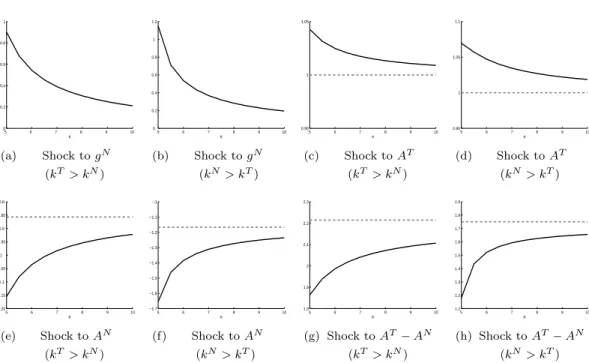
is equal to 1% of output. Figures 1(a)-1(b) report the optimal steady-state response in the relative price to this shock predicted by the model for different values of the parameterθ.14

——————————————————————– <Please insert Figure 1 about here >

——————————————————————–

An important prediction of the model is that the relative price appreciates after a positive shock in domestic government purchases. Figures 1(a)-1(b) substantiate this analytical outcome. Firms selling in non traded markets find it optimal to raise markups because the increase in aggregate demand stemming from the public sector renders the demand for individual goods less price elastic. This generalized rise in domestic markups leads ultimately to an appreciation of the relative price of non traded goods. This prediction of the model is consistent with empirical evidence documenting an increase in relative prices consecutive to an expansion in public consumption (see Froot and Rogoff [1991], De Gregorio et al. ([1994a], [1994b]) and Balvers and Bergstrand [2002]). By contrast, the Balassa-Samuelson setup counterfactually predicts that the relative price is completely unaffected by government spending shocks. Another notable feature in Figures 1(a)-1(b) is that steady-state responses depend on the elasticity of substitutionθ. Not surprisingly, the higher is the value ofθ, the smaller is the markup and the closer are the responses of the relative price to the perfectly competitive model. Indeed, by limiting the transmission of the fiscal shock through the markup, increases in the elasticity of substitution soften the positive response of the relative price to government spending policies.

4.3

Technological shocks

Figures 1(c)-1(f) plot the steady-state response of the relative price of non traded goods to a one percent increase in productivity in sectorT (Figures 1(c) and 1(d)) and in sector N (Figures 1(e) and 1(f)) for different values of the parameterθ. Dotted lines denote the response of the small open economy in which all goods markets are perfectly competitive. It corresponds therefore to the Balassa-Samuelson model or equivalently to equation (21). Solid lines report the response of our imperfectly competitive two-sector framework and capture the total impact of productivity shocks predicted by (22).

13_{For reason of space, we restricted attention to a rise ing}N_{. Numerical results after a fiscal shock ong}T

lead to qualitatively same results and are available from the author upon request. 14_{The responses are shown as percentage deviations from the initial steady state.}

In line with the intuition developed above, the response of the relative price to sector-specific productivity shocks in the Balassa-Samuelson model is insensitive to changes in the price-elasticity of non traded goods. Regardless of the level of the markup, shocks to traded goods productivity by 1% lead to proportional one-for-one relative price appreciations. Pos-itive shocks to TFP in the non traded goods sector result in a fall in the relative price, the extent to which p depreciates depending upon the sectoral capital intensities. For the benchmark calibration ˆp=−0.86% ifkT _{> k}N _{and ˆp=−1.17% ifk}N _{> k}T_{. Now, consider}

instead the steady-state response of the relative price in the present model. As it is apparent in Figures 1(c)-1(f), the qualitative response of the relative price is the same in the model where ˜µN >1 (the solid line) as in the Balassa-Samuelson setup in which ˜µN equals one (the dotted line). However, the quantitative effects depend crucially on markups response. Following a technological shock in the traded sector and for a givenθ, the increase of the rel-ative price is higher under imperfect competition. This result suggests that the inclusion of endogenous market power magnifies the impact of technological shocks in the traded sector on domestic prices via a positive response of markups. By contrast, in response to supply shock in the non traded sector, the model suggests that gains in productivity translate into lower markups and finally into higher relative price reductions. Therefore, a key implica-tion of the model is that part of relative price’s movements triggered by a technological improvement in either the traded or the non traded sector can be attributed to endogenous variations of the markup. Because the latter responses to productivity shifts, in assessing the influence of sector-specific technological shocks on relative prices, it is important to relax the restrictive assumption of perfect competition, and to include goods-markets distortions into the analysis. According to our results, the default to account for the markup induces significant downward-biased estimates of the effects of sector-specific productivity shocks to the relative price of non traded goods. Observe also that the magnitude of the bias (in absolute terms) after productivity gains in the non traded sector is larger than that estimated consecutive to a shock to productivity in the traded sector (28% versus 5% re-spectively for the benchmark).15 _{The reason is that non traded output is more sensitive to}

productivity improvements in sectorN than in sectorT. As a result, the larger variation in YN _{translates into a bigger fluctuation in the composition of demand for non traded goods}

and ultimately into a larger markup change. These model’s properties make two predic-tions about the econometric analysis ran in section 5. First, the endogenous decrease in the markup reinforces the fall in relative price in response to gains in productivity in sector N and hence the coefficient on productivity non tradables would decrease once we net out market power adjustments since the markup captures some of the effects of the productivity improvementsAN_{. Second and by contrast, the productivity of tradables operates relatively}

weakly through the markup channel: its coefficient is expected to be roughly identical when we control for product market competition.

To illustrate further the role of the endogenous markups mechanism in propagating technological shocks, we compute in Figures 1(g)-1(h) the reaction of the relative price to an one percent increase in productivity in sector T relative to sector N (i.e. AˆT ₋

15_{The bias is approximated by (ˆp}BS

−pˆM)/pˆM, where ˆpBS (ˆpM respectively) denotes the relative price percentage deviation from steady-state in the Balassa-Samuelson model (our model respectively).

ˆ

AN _{= 1%). Comparing the magnitude of the response in the model to that observed}

in the standard Balassa-Samuelson framework, we find that the relative price increases by less in the former model. As in the case of sector-specific productivity shocks, the endogenous response of the markup introduces a new and potentially important channel for the transmission of TFP differentials. When the markups adjustment is allowed for, the relative price displays a sensitivity to productivity differentials smaller than in the perfectly competitive framework. Accordingly, the failure to allow for variable markups leads to overstate the Balassa-Samuelson hypothesis in a perfectly competitive framework. This delivers one implication for the following econometric analysis. The coefficient associated with the Balassa-Samuelson term, i.e. the ratio of relative productivity in tradables and nontradables, is expected to be smaller once product market competition is controlled for.

5

Empirical analysis

In this section, we apply the model to study annual data for a panel of thirteen OECD economies over the 1970-2004 period. Having derived testable implications for the relative price of nontradables, our empirical strategy is now to confront the model with the data in the most parsimonious way. We therefore refrain from adding explanatory variables not derived from our model to the regressions. Since most of theoretical priors of the model are based on long-run effects of exogenous real shocks, the cointegration methodology provides a convenient device for testing whether the implications of the model are supported empirically.16 _{Given the relatively short time span (T = 35), it is convenient to apply non}

stationary panel methods to increase the power of tests for unit roots and cointegration.

5.1

Econometric issues

Our theoretical model generalizes the Balassa-Samuelson framework in three ways. First, by accounting for imperfect competition, it predicts that positive fiscal shocks appreciate the relative price of non traded goods in the long-run. Second, technological shocks have ef-fects that are not isomorphic to those obtained from the textbook Balassa-Samuelson setup. This property results from the fact that the markup charged in the non traded sector is also sensitive to gains in productivity. And third, controlling for product market competition, influence of productivity shocks in nontradables and government spending would decrease, while the one associated with productivity gains in the traded sector is expected to be roughly identical. This suggests an empirical strategy that relates relative prices to produc-tivity and fiscal shocks, and where we also search for different impacts of these variables when we control for product market competition. To assess whether these predictions are 16_{This approach allows us to account for non-stationarity in time series of relative prices. For instance,} Canzoneri et al. [1999], Kakkar [2003], Lee and Tang [2007] fail to reject the null hypothesis of a unit root.

supported empirically, regressions of the following form are estimated:

pi,t = θ0i,t+β1bsi,t+εi,t, (24a)

pi,t = θ0i,t+β10bsi,t+β20pmci,t+εi,t, (24b)

pi,t = θ0i,t+γ1bsi,t+γ2govi,t+εi,t, (24c)

pi,t = θ0i,t+γ10bsi,t+γ02govi,t+γ30pmci,t+εi,t, (24d)

whereiandtindex country and time respectively,θ0i,tis a deterministic component (country

fixed effect and/or individual time effect),bsi,tan indicator for the productivity effect,govi,t

is government spending over GDP,pmci,ta proxy for goods market competition (all variables

are converted in natural logarithms) and εi,t is the i.i.d. error term.

Relation (24a) provides the general specification of the Balassa-Samuelson model and relates the relative price to the productivity differentials between the two sectors. We estimate equation (24a) both with and without imposing that the coefficients on productivity in tradables and productivity in non tradables are equal in magnitude and opposite in sign. In the first specification, the relative productivity term enters as a ratio: β1bsi,t =

β1ln(ATi,t/ANi,t). While in the second specification no restrictions on coefficients are imposed:

β1bsi,t=β1TlnATi,t−β1NlnANi,t with a prioriβT1 6=β1N. The theoretical predictions are that

ˆ

β1>0 or ˆβT1 >0 and ˆβ1N >0. Our model provides one refinement to augment the standard

methodology to estimating equation such as (24a). The conventional Balassa-Samuelson approach assumes that productivity shocks, constructed as Solow residuals, are exogenous and uninfluenced by other factors. Indeed, under perfect competition, the Solow residual is identical to the rate of Hicks-neutral technical progress. Due to the presence of market power, it is unlikely, however, that true and measured productivity coincide, meaning that the classical approach to measure productivity gains does not estimate the exact level of technology progress. We therefore eschew conventional TFP measures because, within the present context of imperfect competition, they are not in principle independent of fiscal policy and goods-market competition degree, and on the contrary are crucially affected by them. This drawback of the Solow residual measure motivates our alternative, which we refer to as market power-based Solow residual. This indicator, denoted by mptf pji,t

is constructed by subtracting to the Solow residual (tf pji,t), labor and capital dynamics

(kj_i,t≡ln(K_i,tj /Lj_i,t)) weighted by labor’s share in revenue (αj_i) and markup, as:

mptf pj_i,t =tf pj_i,t−(1−µˆj_i)αj_ikj_i,t, (25) where ˆµji is a proper estimate of the markupµ

j

i andtf p j

i,t is defined as the percent change

in output less the percent change in inputs, where the different inputs are weighted by their factor shares.17 _{Using (25) to estimate technological progress instead of Solow eliminates}

distortions due to the imperfect competition. To make equation (25) operational requires an accurate estimate of markups at the sectoral level. A properly measure of ˆµji is obtained

by applying the consistent Roeger’s [1995] methodology to our sectoral data set.

17_{The derivation of (25) is based on Hall [1988]. His key insight is to show that, under imperfect} com-petition, the Solow residual measures the sum of the pure technology component (aj_i,t) and a labor-capital ratio component (k_i,tj ) in the formtf pj_i,t=aj_i,t+ (1−µj_i)αj_ikj_i,t.

Specification (24b) is a more formal assessment of the theoretical model since it adds to the benchmark regression an important variable of interest in this study, namely, a proxy for product market competition in sector N relative to sector T (pmci,t). This variable

controls for the bias due to the omission of imperfect competition in the Balassa-Samuelson model, that is the effects of technological shocks on the relative price through the markup channel. This alternative regression leads us to evaluate one critical implication of the theoretical analysis. The model predicts that, omitting the product market competition, biases upward the coefficients on the ratio of relative productivities and on productivity on nontradables, confounding the true direct effects of technological shocks on the relative price with the indirect effects through markups variations. By contrast, the model has the stark prediction that productivity gains in the traded sector entail only slight variations in markups. Based on these considerations, we expect that 0 <βˆ0

1 <βˆ1 and 0 <βˆ10N <βˆN1

and we should not expect ˆβ0T

1 to be significantly different from ˆβ1T.18 The equation (24c)

extends further the model by including the fiscal policy variablegovi,t. In light of numerical

results, we hypothesize that ˆγ2>0. Finally, specification (24d) controls for product market

competition in sectorN (relative to sectorT) in regression (24c) and thus, encompasses the strong implications of the theoretical model. Because fiscal shocks influence positively µN

in the model, one should expect markups to be positively correlated with relative prices. Therefore, omitting the product market competition term should bias upward the coefficient ongovi,t. So we expect ˆγ30 >0 and 0<γˆ

0

2<ˆγ2.

5.2

Data

We consider annual data taken from the sectoral KLEMS database. Data covers a maxi-mum period from 1970 through 2004, for a total of thirteen industrialized countries and ten industries.19 _{The country sample consists of Austria, Belgium, Denmark, Spain, Finland,}

France, Germany, Italy, Japan, Netherlands, Sweden, the UK and the US. Following De Gregorio et al. [1994b], Agriculture, Hunting, Forestry and Fishing; Mining and Quarrying; Total Manufacturing; Transport, Storage and Communication are classified as traded goods. Electricity, Gas and Water Supply; Construction; Wholesale and Retail Trade; Hotels and Restaurants; Finance, Insurance, Real Estate and Business Services; and Community Social and Personal Services account for the non traded sector. KLEMS database contains data on value added in current and constant prices, gross output, labor compensation, employ-ment, and capital stock for each sector, permitting the construction of sectoral value-added deflators and the derivation of sectoral TFP and market power-based Solow residual levels. Given that competition cannot be measured directly, proxies of market power in sectorN relative to sectorT (pmci,t) must be used. To this end, we consider two indicators which we

take as reasonable exogenous and have been widely used in the empirical literature.20 _The

two empirical proxies gauge two different concepts of imperfect competition: an indicator measuring profitability (pmc(π)i,t) and a proxy capturing the pricing behavior (pmc(p)i,t).

18_{In addition, another important issue for our estimation purposes is that the variable pmc}

i,t enters

positively in the cointegration vector, i.e. we would expect ˆβ0

2>0.

19_{The data set and construction of variables are described in more details in Appendix A.} 20_{See, among others, Gali [1994], Campa and Goldberg [1995], and Chen et al. [2009].}

Data required for the construction ofpmc(π)i,tandpmc(π)i,tare extracted from the KLEMS

database. Finally, the ratio of government consumption spending to GDP is used to proxy the variablegovi,t (data are obtained from OECD’s National Accounts database).

5.3

Panel unit root tests results

Before turning to the estimation of the models, it may be appropriate to test the stochastic properties of our variables. In order to test for the presence of unit root, we carry out the panel tests proposed by Maddala and Wu [1999] and Im et al. [2003], with results displayed in Table 1. With the exception of productivity in nontradables measured with Solow residuals (tf pN_{), the null hypothesis of a unit root against the alternative of trend stationarity can}

not be rejected at conventional significance levels. By applying the same tests to series in first differences, we strongly reject the null hypothesis of non stationarity in the panel for all series at the 1% significance level, suggesting that all variables are integrated of order one. Taken together, unit root tests applied to the set of variables of interest show that non stationarity is pervasive, making clear that pursue a cointegration analysis is appropriate.

——————————————————————– <Please insert Table 1 about here >

——————————————————————–

To this end, we first implement the Pedroni’s [2004] group parametric-t statistic test to residuals from equations (24a)-(24d) to test for cointegration.21 _{Cointegrating relationships}

are based on the group-mean fully modified OLS (FMOLS) procedure for cointegrated panel proposed by Pedroni ([2000], [2001]). The group-mean FMOLS estimator allows for full endogeneity of the regressors as well as heterogeneity of the dynamics among individuals, and is superconsistent under cointegration. Moreover, the associated t-statistics are distributed as standard normal.

5.4

Traditional estimates

Traditional estimates of the Balassa-Samuelson hypothesis investigate the effects of relative productivities on the relative price of non traded goods using conventional Solow residuals to measure productivity gains. This leads to several specifications, depending on constraints imposed on coefficients on productivity in tradables and non tradables, i.e. whetherAT _and

AN _{enter the regression separately or as a ratio. Table 2 contains the results from estimating}

reduced forms based on (24a).22

——————————————————————– <Please insert Table 2 about here >

——————————————————————–

In all regressions, the Pedroni’s [1999] cointegration test rejects the null hypothesis of no cointegration at the 1% level. In columns (1)-(3), the coefficient on relative productivity 21_{Pedroni [2004] considers seven tests based on the estimated residuals. Four come from pooling data} along the within dimension and three are calculated pooling data along the between dimension. For small time span, Pedroni’s [2004] simulations show that the group parametric-t statistic is the most powerful.

22_{To check the robustness of the results, we consider three alternative ratios: the basic oneA}T_/AN_{, the}

standard Balassa-Samuelson ratio [(AT₎(αN_/αT₎

]/AN_{and the model ratioA}T_/[(AN₎(αT_/αN₎

in tradables and nontradables has the predicted sign and is highly significant. Nonetheless, the Balassa-Samuelson model is not completely successful. Indeed, it predicts not only that p and relative productivities are cointegrated, but also that the slope of the cointegrating vector should be equal to unity. In general, the slope coefficients are fairly precisely estimated and generally close to the unit implied by this model.23 _{However, the regressions in columns}

(1) to (3) are valid only if coefficient estimates on AT _{and A}N _{are similar (in absolute}

terms), this in turn justifies the use of ratios of relative productivity in tradables and non tradables. The results in columns (4) to (6) indicate that the restriction that the coefficients on AT _{and A}N _{are similar in magnitude and opposite in sign is strongly rejected (see the}

second test of coefficient in Table 2). Because the coefficient on productivity in tradables is significantly different from the coefficient on productivity in nontradables (in absolute terms), it is inappropriate to conclude that the Balassa-Samuelson model is successful just because the regressions in columns (1) to (3) suggest a slope close to 1.0. Thus, the data contradict one central prediction of the standard Balassa-Samuelson model that is shocks to TFP differentials are fully transmitted to relative prices.

5.5

Alternatives estimates

Table 3 analyzes the effects of productivity on relative prices for the present model and repeats regressions behind Table 2. Because we are concerned about estimating impacts of productivity differentials on relative prices without measurement errors, regressions (1) to (3) use the market power-based Solow residuals instead of the Solow residuals.

——————————————————————– <Please insert Table 3 about here >

——————————————————————–

For any measure of relative productivity, the cointegration test points to a rejection of the null hypothesis of no cointegration, thus the relative price of non traded goods appears to be cointegrated withmptf pdifferentials. Table 3 also reports the FMOLS estimates of the coefficientβ. These estimates are positive and always statistically significant, implying that differentials in productivity between sectorsT andN appreciate the relative price consistent with model’s prediction. In all specifications, the restriction that the coefficient on the productivity term is equal to unity is strongly rejected at conventional levels. Although the econometric analysis fails to obtain a unit cointegrating vector, it is premature to view this drawback as a basis for rejecting the model. Indeed, the present framework suggests that an increase in the relative productivity differential appreciates the relative price, but, to the extent that markups also respond to sector-specific productivity shocks, it does not predict that the two variables are proportional in the long-run. Moreover, tests of coefficients equality in columns (4) to (6) suggest that perfect symmetry in the effects of tradables and nontradables productivities is rejected at standard confidence levels. Hence, there is strong evidence that the coefficient estimates on productivities in sectors T and N have different magnitudes (as predicted by the model) when using the market power-based Solow 23_{See the first test of coefficient on the bottom half of Table 2 which shows that the evidence in favor of} the restrictionβ= 1.0 is quite strong in columns (1) and (2).

residuals measure. In an attempt to assess the importance of the choice of the productivity measure, the last row of Table 3 reports the p-values of the restriction that the coefficients

estimated from the Balassa-Samuelson model ( ˆβBS_{, see Table 2) and those estimated in the}

model ( ˆβM_{) are equal in magnitude. In all specifications, these coefficients are significantly}

different. Hence, tf p and mptf p measures are not interchangeable. This result reflects the inherent difference between two measures of productivity gains used. In particular,tf p proxy is not exogenous to imperfect competition and investment and labor dynamics, while mptf p is free from the possibly endogenous variations in these variables. One implication of this is that standard estimates of the Balassa-Samuelson effect usingtf p data are likely to be biased due to a measurement error in Solow residuals.24

The results in Tables 2 and 3 suggest also that the outstanding specification is the one in which productivity terms in tradables and non tradables enter separately since coefficients on AT _{and A}N _{cannot be constrained to be equal in magnitude. Hence, our benchmark}

specification, in what follows, includes productivity terms separately and bothAT _andAN

are measured with mptf p (see column (4) in Table 3). This specification is expanded in Table 4 to incorporate the effects of fiscal policy and market product competition on the relative price. This approach allows a strict test of the model’s implications. For comparison purpose, column (1) simply restates the benchmark regression (4) in Table 3. FMOLS results suggest that a 1% increase in productivity in the traded sector raises the relative price by 0.77%, while a 1% shock to nontradables productivity leads to a fall in p by 0.95%.25

Regressions in columns (2) to (6) are the empirical counterparts to theoretical equations (24b), (24c) and (24d). Two aspects of the results support the present model.

——————————————————————– <Please insert Table 4 about here >

——————————————————————–

First, the coefficient on the market product competition proxy has the correct sign and is significant at the one percent level. In other words, low competition degree in non traded sector (relative to sector T) exerts an upward pressure on relative prices of non traded goods. According to the two first tests of coefficients’ equality displayed in the bottom half of Table 4, the competition variable also reduces greatly and significantly the size of the coefficient on productivity in nontradables while the coefficient on AT _{is statistically}

unaffected by the presence of the competition measure as the model would have predicted. This stresses the importance of controlling for imperfect competition when estimating the influence of productivity shocks on relative prices. To the extent that non traded firms have a substantial market power, the response of markups to an increase in AN _{erodes the}

benefits of disinflation effects associated with positive technological shocks in that sector. Less competitive economies tend, therefore, to experience higher nontradables inflation since the transmission mechanisms of positive shocks to productivity in sector N into relative price reductions are weaker. It is also interesting to note that the estimated biases due to 24_{The biases introduced by measurement error can be rather severe, especially with fixed effect estimates.} See Griliches and Hausman [1986] and references therein.

25_{These estimates are not directly comparable with those found in the previous literature, because of the} different productivity measures employed.

the failure to allow for imperfect competition are in a similar order of magnitude to those computed from the theoretical model. The differences in the estimated coefficients on AT

andAN _{in regressions which include the product competition term (columns (2) to (3)) and}

estimates of the basic model without this variable (regression (1)) represent the outcome of the bias. On the basis of these estimates, we find that the bias reaches 4% for for shocks to AT _{and 24% for for shocks to A}N_{. These values are consistent with numerical calculations}

which provide theoretical biases equal to 5% forAT _{and 28% forA}N_.

Second, the coefficient on fiscal policy, in regressions (4) to (6), has the predicted sign and is highly significant. These point estimates suggests that an one percentage point shock to the share of government expenditure increases the relative price of nontradables by 0.32 to 0.60 percent. These results accord with the qualitative predictions of the theoretical analysis. One another important aspect of the model is that goods market competition degree affects also the strength of effects of fiscal policy on the relative price. This prediction is tested and confirmed in columns (5) and (6) which reports the results from regressing the relative prices on sectoral productivities, government spending and market product competition. In both cases, the coefficient on fiscal policy is significantly lower from the one obtained in the regression (4) without competition proxy.

6

Conclusion

This paper calls into question the conventional wisdom that relative price trends observed in industrialized countries are entirely governed by the response of economy’s supply-side to divergence of productivity levels in traded and non traded goods sectors. On the theo-retical side, we provide a reappraisal of the static theory of Balassa [1964] and Samuelson [1964] by embedding their approach in an explicitly dynamic general equilibrium setting featuring monopolistic competition and endogenous markups. In such framework, markups vary in response to shifts in the composition of demand for non traded goods and optimal intertemporal plans of households and government’s decisions have the potential to affect the relative price of nontradables. The model emphasizes therefore the role of markups in the propagation of macroeconomic shocks implying that responses of the relative price to both technological and fiscal disturbances into the framework have little in common with those observed in the classical Balassa-Samuelson economy. First, the presence of endoge-nous markups is shown to make fiscal policy non-neutral. Second, the effects of productivity shocks are not analogous to those derived in the Balassa-Samuelson setting, suggesting that the latter framework tends to misidentify the influence of sector-specific productivity shocks. The empirical part of the paper converts the model into a form that is directly amenable to econometric analysis. In particular, we check whether the imperfect competition hy-pothesis (and its resulting outcomes) affects the relative price of nontradables in a manner consistent with theory. The econometric results illustrate the robustness of the theoretical findings. First, we show that, for an appraisal of the Balassa-Samuelson effect, the choice of the productivity measure can lead to different conclusions regarding the performance of the underlying model. Based on Solow residuals to proxy efficiency gains, the textbook Balassa-Samuelson hypothesis is not completely successful. By contrast, the market power-based

Solow residuals seem to be the more appropriate and preferred measure of productivity gains, being exogenous from influence of endogenous variations in markups. Moreover, our estimations highlight that the failure to control for imperfect competition induces substan-tial biases in the effects of productivity shocks to nontradables on the relative price. And second, we stress the importance of additional real factors influencing relative prices in the long-run. In particular, our empirical findings point out the potential disinflation gains originating from deregulation policies, while, in contrast, expansive fiscal policies tend to fuel nontradables inflation. On the whole, the paper’s theoretical and empirical findings underscore that one must go beyond the textbook Balassa-Samuelson framework to capture overall dynamics of relative prices over time and across countries.

A

Appendix: data construction

In what follows, subscript i refers to country, k industry, t time and j sector (j =T, N). Define value-added measured at current prices (V A) and value-added volume (V AV) for sector j, countryi as V Aj_i,t =P

k∈j V A j k,i,t and V AV j i,t = P k∈j V AV j k,i,t,where V A j k,i,t

(V AV_k,i,tj resp.) is the value-added measured at current prices (value-added volume resp.) for industrykclassified in sectorj. All prices are value-added deflators: P_i,tj =V Aj_i,t/V AV_i,tj. The relative price of non traded goods for countryi is therefore defined byPi,t=Pi,tN/Pi,tT.

Productivity indexes are computed by averaging industry-specific indicators with a weight-ing scheme based on the share of each industrykin the total value added of the sectorj. To-tal factor productivity index for sectorjis therefore given byT F P_i,tj =P

k∈j ω j

k,i,tT F P j k,i,t,

whereT F P_k,i,tj is the TFP for industrykclassified in sectorjand where the weights (ωj_k,i,t) are based on the size of value-added of each industry k, that is ω_k,i,tj =V Aj_k,i,t/V Aj_i,t for k∈j. Total factor productivity index for industry k is computed assuming Cobb-Douglas production functions: T F Pk,i,tj = V AV

j k,i,t/[(L j k,i,t) αj k,i_(Kj k,i,t) 1−αj k,i_{], where L}j k,i,t (K j k,i,t

resp.) is the total employment (capital resp.) andαj_k,i is labor share in total income aver-aged over the period 1970-2004 in industryk.

We compute the market power-based Solow residual, denoted byM P T F Pk,i,tj , by

em-ploying a two-step estimation strategy. The first step consists in estimating a markup over marginal costs in industryk classified in sectorj. For this purpose, we apply the Roeger’s [1995] methodology which requires to estimate the following equation:

zj_k,i,t=δj_k,iwj_k,i,t+uj_k,i,t, (A1) withzjk,i,t= ∆GO j k,i,t−ϕ j k,i,t∆COM P j k,i,t−υ j k,i,t∆M I j k,i,t−(1−ϕ j k,i,t−υ j

k,i,t)∆(ri,tKk,i,tj ),

and w_k,i,tj = ∆GOj_k,i,t−∆(ri,tK_k,i,tj ). ϕj_k,i,t and υ_k,i,tj are the shares of labor and

mate-rials costs in the value of gross output respectively. ∆GOj_k,i,t denotes the nominal out-put growth, ∆M I_k,i,tj the growth in nominal intermediate input costs and ∆(ri,tKk,i,tj )

the nominal capital cost growth for industry k classified in sector j. All these variables are compiled from the KLEMS database except the user cost of capital ri,t. No

sector-specific information is available to construct ri,t, so the rental price of capital is estimated

with ri,t =pIi,t ii,t−πi,tGDP +δ

, where pI

i,t is the deflator for business non residential

rate and the depreciation rate δ is fixed at 5% throughout (pI

i,t, ii,t and πGDPi,t are taken

from OECD databases). To tackle the potential endogeneity of the regressor and the het-eroskedasticity and autocorrelation of the error term, equation (A1) is estimated by using heteroskedastic and autocorrelation consistent standard errors as suggested by Newey and West [1993] (lag truncation = 2). The markup estimate in industry k classified in sector j, namely ˆµj_k,i, is equal to 1/(1−ˆδ_k,ij ). Markup indexes of traded and non traded sectors for country i are assessed as follows ˆµji =

P k∈j ω j k,i µˆ j k,i, where ω j

k,i stands for the

pe-riod average share of industry k in the total value-added of the sector j. A special note should be made for ”Community Social and Personal Services” industries. Output in this industry is produced to a significant extent by non-market producers (government or other non-profit firms). Therefore, estimates of the markup for those industries might not be always meaningful and we do not take into account ”Community Social and Personal Ser-vices” when calculating markups for the non traded goods sector ˆµN

i . In the second step,

we use the estimated markups ˆµj_k,i to construct the market power-based Solow residual as M P T F P_k,i,tj = T F P_k,i,tj (K_k,i,tj /L_k,i,tj )(1−αj_k,i)(ˆµj_k,i−1)_{. Market power-based Solow residual}

for sector j is therefore given byM P T F P_i,tj =P

k∈j ω j

k,i,tM P T F P j k,i,t.

Regarding the demand side-effect, we use the ratio of government consumption spending to GDP:GOVi,t=GSi,t/GDPi,t, whereGSi,tdenotes government consumption expenditure

and GDPi,t is the gross domestic product of country i. We consider two empirical proxies

for product market competition: a proxy measuring profitability and a proxy capturing the pricing behavior. The profitability measure for sector j is given by comp(π)j_i,t = (GO_i,tj −

M_i,tj −COM P_i,tj )/GOj_i,t. The pricing behavior index is calculated as the inverse of the labor income share (excluding the imputed labor income of the self-employed) in sectorj: comp(p)ji,t = (V A j i,t/N j i,t)/(COM P j i,t/L j

i,t), where total employees (N j

i,t) and employment

or equivalently persons engaged (Lj_i,t) used in sector j are given by N_i,tj = P

k∈j N j k,i,t and Lji,t = P k∈j L j k,i,t where N j k,i,t (L j

k,i,t resp.) is total employees (employment resp.)

in industry kclassified in sector j. To be consistent with the general lessons of the model, the product market competition indicator (P M Ci,t) is rescaled according to: P M C(π)i,t=

comp(π)N

i,t/comp(π)Ti,t and P M C(p)i,t = comp(p)Ni,t/comp(p)Ti,t. A rise in P M C(π)i,t (or

P M C(p)i,t) indicates that the market power in sectorN increases relative to that observed

in the traded sector.

By using the translation of notationsxi,t= logXi,t, we then obtain the variables involved

in regressions (24): pi,t,tf pi,t,mptf pi,t, govi,t,pmc(π)i,t andpmc(π)i,t.

References

Balassa B. (1964), “The Purchasing Power Parity Doctrine: a Reappraisal”,Journal of Political Economy, vol. 72, 584-596.

Balvers R.J. and J.H. Bergstrand (2002), “Government Expenditures and Equilibrium Real Exchange Rates”,Journal of International Money and Finance, vol. 21, 667-692.

Bergin P.R., R. Glick and A.M. Taylor (2006), “Productivity, Tradability, and the Long-Run Price Puzzle”,Journal of Monetary Economics, vol. 53(8), 2041-2066.

Bettendorf L.J.H. and B.J. Heijdra (2006), “Population Ageing and Pension Reform in a Small Open Economy with Non-Traded Goods”,Journal of Economic Dynamics and Control, vol. 30, 2389-2424.