Distributed Response Time Analysis of GSPN Models with MapReduce
Oliver J. Haggarty William J. Knottenbelt Jeremy T. BradleyDepartment of Computing, Imperial College of Science, Technology and Medicine, 180 Queen’s Gate, London, SW7 2BZ, United Kingdom
{ojh06, wjk, jb}@doc.ic.ac.uk
Abstract
Generalised Stochastic Petri nets (GSPNs) are widely used in the performance analysis of computer and communica-tions systems. Response time densities and quantiles are of-ten key outputs of such analysis. These can be extracted from a GSPN’s underlying semi-Markov process using a method based on numerical Laplace transform inversion. This method typically requires the solution of thousands of systems of complex linear equations, each of rank n, where n is the num-ber of states in the model. For large models substantial pro-cessing power is needed and the computation must therefore be distributed.
This paper describes the implementation of a Response Time Analysis module for the Platform Independent Petri net Editor (PIPE2) which interfaces with Hadoop, an open source implementation of Google’s MapReduce distributed programming environment, to provide distributed calculation of response time densities in GSPN models. The software is validated with analytically calculated results as well as simu-lated ones for larger models. Excellent scalability is shown.
1
INTRODUCTION
The complexity of computer systems continues to rise rapidly. It is therefore increasingly important to model sys-tems prior to their implementation to ensure they behave correctly. In this context, Generalised Stochastic Petri nets (GSPNs) are a popular graphical modelling formalism which are both intuitive and flexible. GSPNs have an underlying semi-Markov process which can be analysed for many quali-tative and quantiquali-tative factors.
The focus of the present paper is on techniques for extract-ing response time densities and quantiles from GSPN models. Given their increasing use in Service Level Agreements, these are important performance measures for many computer and communication systems, such as web servers, communica-tion networks and stock market trading systems. In particular, we describe the creation of a new Response Time Analysis module for the Platform Independent Petri net Editor (PIPE2) [3]. PIPE21is an open source Petri net editor and analyser de-veloped by several generations of students at Imperial College London as well as several external contributors. The module accepts a set of start and target markings (defined by logical
1Available fromhttp://pipe2.sourceforge.net.
expressions which describe the number of tokens that should be present on selected places) and outputs graphs of the cor-responding response time density and (optionally) the cumu-lative distribution function of the time taken for the system to pass from the start markings into any of the target mark-ings. The analysis makes use of a method based on numerical Laplace transform inversion, whereby we convolve the state sojourn times along all paths from the set of start markings to the target markings [6]. This involves the solution of many systems of complex linear equations, each of rank n, where n is the size of the GSPN’s state space. For large n the calcula-tions require a great deal of processing power. Consequently, we distribute the processing over a cluster of computers by interfacing PIPE2 with Hadoop, an open source implemtation of Google’s MapReduce distributed programming en-vironment. This paradigm offers excellent scalability and ro-bust fault tolerance.
The remainder of this paper is organised as follows. Sec-tion 2 presents relevant background material relating to Gen-eralised Stochastic Petri nets and their response time analysis. Section 3 describes Hadoop, an open source implementation of the MapReduce distributed programming model. Section 4 describes the design and integration of an Hadoop-based Re-sponse Time Analysis module into the PIPE2 Petri net edi-tor. Finally, Section 5 validates the module using small mod-els with known analytical results, as well as larger modmod-els where results had been produced by simulation. The software is shown to work with model sizes with in excess of two mil-lion states, and to scale well with increasing analysis cluster size. Section 6 concludes.
2
BACKGROUND THEORY
Petri nets are a graphical formalism for describing con-currency and synchronisation in distributed systems. In their simplest form, they are also known as Place-Transition nets. These consist of a number of places, which may contain to-kens, connected by transitions. A transition is enabled and can fire if the input places of the transition contain at least the number of tokens specified by a backward incidence ma-trix. In so firing, a number of tokens are removed from the transition’s input places and a number of tokens added to the transition’s output places according to the backward and for-ward incidence matrices respectively.
number of tokens on each place of the model. The
reacha-bility set or state space of a Place-Transition net is the set of
all possible markings that can be reached from a given ini-tial marking. The reachability graph shows the connections between these markings.
Generalised Stochastic Petri nets (see e.g. Figures 4 and 5) extend Place-Transition nets by incorporating timing infor-mation. A timed transition tihas an exponentially distributed
firing rateλi. Immediate transitions have priority over timed transitions and fire in zero time. Markings that enable timed transitions only are known as tangible, while markings that enable any immediate transition are called vanishing. The sojourn time in a tangible marking Mi is exponentially
dis-tributed with parameter µi=∑k∈en(Mi)λkwhere en(Mi)is the
set of transitions enabled by marking Mi. The sojourn time in
vanishing markings is zero. Formally, [2]:
Definition 2.1 A Generalised Stochastic Petri net is an
8-tuple GSPN= (P,T,I−,I+,M0,T1,T2,W). P={p1, ...,p|P|}
is a finite and non-empty set of places T ={t1, ...,t|T|} is a
finite and non-empty set of transitions. P∩T = /0. I−,I+:
P×T →N0are the backward and forward incidence
func-tions, respectively. M0: P→N0is the initial marking. T1⊆T
is the set of timed transitions. T2⊂T is the set of immediate
transitions; T1∩T2=/0and T =T1∪T2. W = w1, ...,w|T|
is an array whose entry wi∈R+is either a rate of a
nega-tive exponential distribution specifying the firing delay, when
transition ti is a timed transition, or a firing weight, when
transition tiis an immediate transition.
We further define pi j to be the probability that Mj is
the next marking entered after marking Miand, for tangible
marking Mi, qi j=µipi j, i.e. qi jis the instantaneous transition
rate into marking Mjfrom marking Mi.
2.1
Response Time Analysis using Numerical
Laplace Transform Inversion
If we first consider a GSPN whose state space does not contain any vanishing states, the definition of the first passage time from a single source marking i to a non-empty set of target markings~j is given by:
Ti~j=inf{u>0 : M(u)∈~j,N(u)>0,M(0) =i}
where M(u)is the marking of the GSPN at time u and N(u)
is the number of transitions which have fired by time u. When studying GSPNs whose state spaces include vanish-ing states we define the passage time as:
Ti~j=inf{u>0 : N(u)≥Mi~j}
where Mi~j=min{m∈Z+: Xm∈~j|X0=i}; here Xmis the
state of the system after the mth transition firing [4].
To find this passage time we must convolve the state so-journ time densities for all paths from i to j∈~j. This is best
done in the Laplace domain as we can take advantage of the convolution property which states that the convolution of two functions is equal to the product of their Laplace transforms. We perform a first-step analysis to find the Laplace transform of the relevant density. This process can be thought of as first finding the probability density of moving from state i to its set of direct successor states~k and then convolving it with
the probability density of moving from~k to the set of
tar-get states~j. Vanishing markings have a sojourn time density
of 0, with probability 1, which results in their Laplace trans-form equalling 1 for all values of s. If
L
i~j(s)is the Laplace
transform of the density function fi~j(t)of the passage time
variable Ti~j, then we can express
L
i~j(s)as:L
i~j(s) = ∑
k∈/~j q ik s+µiL
k~j(s) +∑
k∈~j q ik s+µi if i∈T
∑k/∈~jpikL
k~j(s) +∑k∈~jpik if i∈V
where
T
is the set of tangible markings andV
is the set of vanishing markings.This system of linear equations can also be expressed in matrix–vector form. If, for example, we wish to find the pas-sage time from state i to the set of states~j={M1,M3},where
T
={M1,M3, . . . ,Mn}andV
={M2}, then: s−q11 −q12 0 · · · −q1n 0 1 0 · · · −p2n 0 −q32 s−q33 · · · −q3n 0 . . . 0 . .. ... 0 −qn2 0 · · · −qnn L= q13 p21+p23 q31 . . . qn1+qn3 (1) where L= (L
1~j(s), . . . ,
L
n j(s)). If we wish to calculate thepassage time from multiple source states, denoted by the
vec-tor~i, the Laplace transform of the passage time density is
given by:
L
~ i~j(s) =∑
k∈~i αkL
k~j(s)where αk is the steady-state probability that the GSPN is in state k at the starting instant of the passage.αkis given by:
αk=
πk
/∑n∈~iπn if k∈~i
0 otherwise (2)
where πk is the kth element of the steady-state probability vectorπof the GSPN’s underlying embedded Markov Chain. Now that we have the Laplace transform of the passage time, we must invert it to get the density of interest in the real domain. To do this we can use Euler inversion [1]. This works by evaluating the Laplace transform f∗(s)at various s-values determined by the value(s) of t at which we wish to evaluate
f(t). From these results it approximates the inverse Laplace transform of f∗(s), i.e. f(t). Formally:
f(t)≈e A/2 2t Re f∗ A 2t +e A/2 2t ∞
∑
k=1 (−1)kRe f∗ A+2kπi 2t (3)where A=19.1 is a constant that controls the discretisation error. This equation describes the summation of an alternat-ing series, the convergence of which can be accelerated by employing Euler summation.
3
THE MAPREDUCE ENVIRONMENT
MapReduce was devised by Google researchers Dean and Ghemawat as a programming model, with an associated im-plementation, to facilitate the generation and processing of large data sets on clusters of commodity machines [5]. It was intended to allow reliable and efficient distributed programs to be written by developers with little prior experience of writing distributed applications.
The framework presented to the developer is inspired by primitive functions of the Lisp programming language, whereby computations are split into a Map task and a Reduce task, both of which the developer is responsible for writing. The Map function takes a series of input key/value pairs and produces a set of intermediate key/value pairs. The MapRe-duce framework then collects together all intermediate pairs with the same key and passes the collection to the Reduce function. This then takes one such pair consisting of a single key and a list of values and processes the values in such a way that it will produce zero or one output value(s). This is the output along with the intermediate key as a key/value pair. We can summarise this as:
Map(k1,v1) → list(k2,v2)
Reduce(k2,list(v2)) → (k2,v2)
It should be noted that the typing of the keys and values is important. The input keys and values can be from a different domain to the intermediate keys and values (i.e.k1andk2
can be different types). However, the intermediate keys and values must be of the same type as the output keys and values.
3.1
Hadoop Implementation
There are a number of implementations of Google’s MapReduce programming model, including Google’s own, written in C++ and discussed in [5]. Different implementa-tions can be tailored for the systems they are intended to run on, such as large networks of commodity PCs or powerful, multi-processor, shared-memory machines. In this section we will introduce Hadoop, an open-source Java implementation of the MapReduce model.
Hadoop consists of both the MapReduce framework and the Hadoop Distributed File System (HDFS), reminiscent of the Google File System (GFS). A distributed filesystem uses the local drives of networked computers to store data whilst making it available to all machines connected to the network. Hadoop is designed to be run on large, extensible clusters of
commodity PCs and has been demonstrated to run on clusters of up to 2000 machines.
HDFS consists of three main processes: the Namenode, the Secondary Namenode and a number of Datanodes. The Namenode runs on a single master machine in the cluster and stores details of which machines make up the cluster and where each block is stored on which machines. It also handles replication. The Secondary Namenode is an optional back-up process for the Namenode. Datanode processes run on all other machines in the cluster (slaves). They communi-cate with the Namenode and handle requests to store blocks of data on the machine’s local hard disk. They also update the Namenode as to the location of blocks and their current status.
The MapReduce framework is comprised of a single Job-Tracker and a number of TaskJob-Trackers. The JobJob-Tracker pro-cess runs on a single, master machine (often the same as the Namenode) and can be thought of as the controller of the clus-ter. Users submit their MapReduce jobs to the JobTracker, which then splits the work between various machines in the cluster. A TaskTracker process runs on each machine in the cluster. It communicates with the JobTracker and is assigned Map or Reduce tasks when it is available.
3.2
MapReduce Job Execution Overview
In order to give a clear picture of how Hadoop works we shall now describe the execution of a typical MapReduce job on the Hadoop platform. When the user submits their MapRe-duce program to the JobTracker the first step is to split the input data (often consisting of many files) into M splits of be-tween 16 and 128 MB in size. There are M Map tasks and
R Reduce tasks per job; both values can be specified by the
user. When a TaskTracker receives an instruction to run a Map task from the JobTracker it spawns a TaskTrackerChild pro-cess to carry out the work. It then continues to listen for fur-ther instructions, fur-thereby allowing multiple tasks to be run on multiprocessor or multicore machines. The TaskTracker-Child’s first step is to read a copy of the task’s associated input split from the HDFS. It parses this for key/value pairs before calling the Map function for each pair. After perform-ing some user defined calculations, the Map function writes intermediate key/value pairs to the local disk. There are typi-cally many of these per Map. These pairs are partitioned into
R regions, each region containing key/value pairs for a subset
of the keys. At the end of the Map task the TaskTracker in-forms the JobTracker it has completed its task and gives the location of the intermediate pairs it has created.
A TaskTracker that has been assigned a Reduce task will copy all the intermediate pairs from a single partition region to its local disk. These pairs will be distributed amongst the local disks of all workers that have run a Map task. Once copied, it sorts the pairs on their keys. A call to the Reduce
function is made for each unique key and the list of associ-ated values is passed in. The output of the reduce function is appended to an output file associated with the Reduce task. R output files will be produced per job.
It is often the case that a single Map task will produce many key/value pairs with the same key. Ordinarily, these will all need to be individually copied to the machine running the cor-responding Reduce task. However, to reduce network band-width the MapReduce framework allows a Combiner func-tion to be run on the same machine that ran the Map task, which partially merges intermediate data before it is trans-ferred. Network bandwidth is further reduced by taking ad-vantage of replication within the HDFS, whereby each block of data is stored on a number of local disks for fault tolerance reasons. When a machine requires some data the Namenode gives it the location on the machine storing the data which is closest on the network path. The MapReduce framework further takes advantage of this property by attempting to run Map tasks on machines that are already storing a copy of the corresponding file split on their local disk.
The key mechanism for handling failure of nodes in the MapReduce cluster is re-execution. While the JobTracker is a very important part of the system and is a single point of failure, the chances of that one machine failing are low. Hadoop therefore currently does not have any fault tolerance procedures for it and the entire job must be re-executed. In a large cluster of slaves the chances of a node failing are much higher. To counter this, the JobTracker periodically pings each TaskTracker. If it does not receive a response within a certain time it marks the node as failed and re-schedules all Map tasks carried out by that node since the job started. This is necessary as the intermediate results for those tasks will be stored on that node’s local hard-disk, which is now inaccessi-ble. This allows a job to continue with minimal re-execution.
4
PIPE2 RESPONSE TIME ANALYSIS
The Platform Independent Petri net Editor (PIPE) was cre-ated in 2002 at Imperial College London as a group project for MSc (Computing Science) students. The motivation was to produce an intuitive Petri net editor compliant with the latest XML Petri net standard, the Petri Net Mark-up Lan-guage (PNML). Subsequent projects and contributions from external developers have extended the program to version 2.5, adding support for GSPNs, further analysis features and im-proved GUI performance [3]. An important feature of PIPE2 is the facility for pluggable analysis modules. That is, an ex-ternally compiled analysis class can be dropped into a Mod-ule folder and the ModMod-uleLoader class then uses Java reflec-tion to integrate it into the applicareflec-tion at run-time. All module classes must implement a predefined Module interface:
public void run(PNMLData petrinet) { ... }
public String getName() { ... }
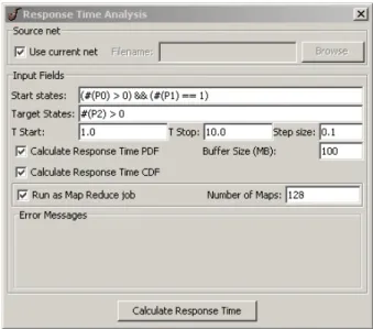
Figure 1. User-facing input window of the PIPE2 Response
Time Analysis module
Existing modules support tasks such as steady-state analy-sis, reachability graph visualisation and invariant analysis. A number of other modules are also currently being developed.
4.1
Overview of Module
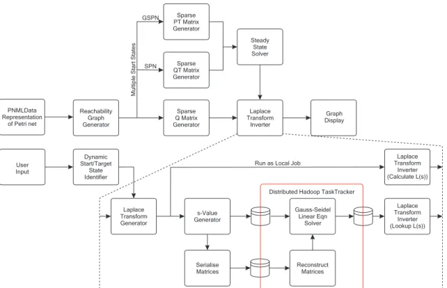
Figure 1 shows the user-facing input window of the PIPE2 Response Time Analysis module, while Figure 2 shows a breakdown of the steps which the module takes in order to calculate response time densities for a GSPN model. The module can be seen to take the representation of the Petri net as a PIPE2 PNMLData object and use this to generate the various matrices required for the calculation of the response time density. The user is allowed to input logical expressions to identify sets of start and target markings. Next, the reach-ability graph (described as the generator matrix Q in the case of an SPN and as an EMC with probability transition matrix P in the case of a GSPN) is generated and the steady-state prob-ability distribution vector is calculated (recall this is required to weight start states appropriately). The Laplace transform inverter can be run either locally or in distributed format us-ing the Hadoop MapReduce platform. Distributus-ing the LT in-verter allows for large models to be analysed in a scalable manner in reasonable time.
The first step in the Laplace transform inverter is to gen-erate the complex linear systems that must be solved to yield the Laplace transform of the convolution of all state sojourn times along all paths from the set of start markings to any of the set of target markings. These are calculated as described in Section 2.1 and are dependent on the target states recog-nised by the start/target state identifier. The number of linear systems to be solved depends on the number of time points specified by the user; these systems are then solved either
lo-Figure 2. Overview of Response Time Analysis module
cally or as a distributed MapReduce job on Hadoop. Finally, the results are displayed as a graph whose underlying data can be saved as CSV file.
4.2
Reachability Graph Generator
The reachability graph genenerator used in the Response Time Analysis module is based on an existing one already implemented in PIPE2 by [7]. Its concept is to perform a breadth-first search of the states of the GSPN’s underlying SMP. It starts with a single state and finds all the states that can be reached from it in a single transition. This process is then repeated for each of those successor states until all states have been explored. In order to detect cycles a record must be kept in memory of each state identified; this presents a sig-nificant problem when dealing with large state spaces. Stor-ing an array representStor-ing the markStor-ing of each state’s places would consume far too much memory. A better approach is to employ a probabilistic, dynamic hashing technique, as de-vised in [8]. Here, only a hash of the state’s marking array is stored in one of many linked lists which are in turn stored in a hash table. By using a second hash function to determine which list to store each state in the risk of collisions is dra-matically reduced. A full representation is also stored on disk as it is necessary when identifying start and target states. The new I/O classes introduced in Java J2SE 5 were used to dra-matically improve performance when writing to disk.
4.3
Dynamic Start/Target State Identifier
A passage time of interest can be specified by defining a set of start states and a set of target states. For example, a user might wish to calculate the passage time from any state where a buffer contains three items, to any state where it con-tains none. In Petri net modelling the buffer would correspond to a place while the items would be tokens. A convenient way for the user to be able to specify sets of start and target states is by giving conditions on the number of tokens on places. Finding the corresponding states is a non-trivial problem as the entire state space must be searched to identify such states. A very fast algorithm is required as state spaces can be huge. We accomplish this by allowing the user to enter a logical ex-pression, whose terms compare the markings of places with constants or the markings of other places. This is then trans-lated into a Java expression which is inserted into a template that is compiled and invoked at run-time to check whether each state matches the user’s conditions.
4.4
Steady-State Solver
The steady-state solver uses the Gauss-Seidel iterative method to find the steady-state distribution vector of a Markov chain represented by a Q (or P) matrix by solving the equationπQ=0 (orπP=π). To obtain standard linear sys-tem form Ax=b requires the transpose of the Q or P matrix,
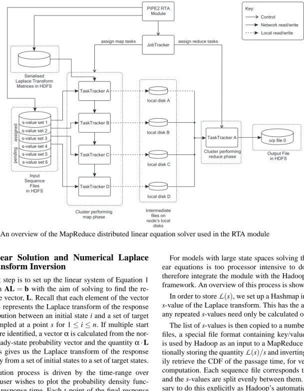
Figure 3. An overview of the MapReduce distributed linear equation solver used in the RTA module
4.5
Linear Solution and Numerical Laplace
Transform Inversion
The next step is to set up the linear system of Equation 1 of the form AL=b with the aim of solving to find the
re-sponse time vector, L. Recall that each element of the vector
Li=
L
i~j(s)represents the Laplace transform of the responsetime distribution between an initial state i and a set of target states~j sampled at a point s for 1≤i≤n. If multiple start
markings are identified, a vectorαis calculated from the nor-malised steady-state probability vector and the quantityα·L
found. This gives us the Laplace transform of the response time density from a set of initial states to a set of target states. The solution process is driven by the time-range over which the user wishes to plot the probability density func-tion of the response time. Each t-point of the final response time distribution requires 65 s-point function calls (in this im-plementation) of the Laplace transform of the response time density. Each s-point sample of the Laplace transform is given by a single solution of Equation 1. The precise set of s-values required are calculated from the Euler Laplace inversion al-gorithm as a function of the desired time range of the final plot. Thus a time range of 100 points may require as many as 6500 distinct solutions of Equation 1, provided by a standard Gauss-Seidel iterative method
For models with large state spaces solving the sets of lin-ear equations is too processor intensive to do locally. We therefore integrate the module with the Hadoop MapReduce framework. An overview of this process is shown in Figure 3. In order to store
L
(s), we set up a Hashmap indexed on thes-value of the Laplace transform. This has the advantage that
any repeated s-values need only be calculated once.
The list of s-values is then copied to a number of sequence files, a special file format containing key/value pairs which is used by Hadoop as an input to a MapReduce job. By addi-tionally storing the quantity
L
(s)/s and inverting, we caneas-ily retrieve the CDF of the passage time, for very little extra computation. Each sequence file corresponds to a Map task and the s-values are split evenly between them. It was neces-sary to do this explicitly as Hadoop’s automatic file splitting functionality is aimed at much larger data files.
The set of A-matrices corresponding to a set of the required
s-values are serialised and the resulting binary file is copied
into the cluster’s HDFS. When a node receives a Map task it will run the Map function a number of times; once for each s-value in its associated sequence file. For the first Map function run on a node, the A-matrices are copied out of the HDFS to local storage and deserialised. Subsequent calls to the Map function (even as part of different Map tasks) then use this
local copy, thereby greatly reducing network traffic.
Whilst the
L
(s)values are being calculated, a single Re-duce task is started. We use the ReRe-duce task simply to collect all theL
(s)values from across the cluster and copy them toa single output sequence file. With the distributed job com-plete, the response time calculator copies the results into a HashMap indexed on s-values for fast access and runs the Euler algorithm.
5
NUMERICAL RESULTS
All results presented in this section were produced by PIPE2 running in conjunction with the latest development version of Hadoop (0.13.1) on a cluster of 15 Sun Fire x4100 machines, each with two dual-core, 64-bit Opteron 275 pro-cessors and 8GB of RAM. The operating system is a 64-bit version of Mandrake Linux and nodes are connected by giga-bit ethernet and an Infiniband interface managed by a Silver-storm 9024 switch with a throughput of 2.5Gbit/s. One of the nodes was designated the master machine and ran the Hadoop Namenode and JobTracker processes, as well as PIPE2.
5.1
Validation
Our validation process began with the Branching Erlang model, taken from [9] and shown in Figure 4, which con-sists of two branches with known response times. In particu-lar, the upper branch has an Erlang(12,2)distribution, while the lower has an Erlang(3,1)distribution. There is an equal probability of either branch being taken, as the weights of the immediate transitions are identical. As Erlang distributions are trivial to calculate analytically we can therefore compare the results form our numerical Laplace transform inversion method with their true values.
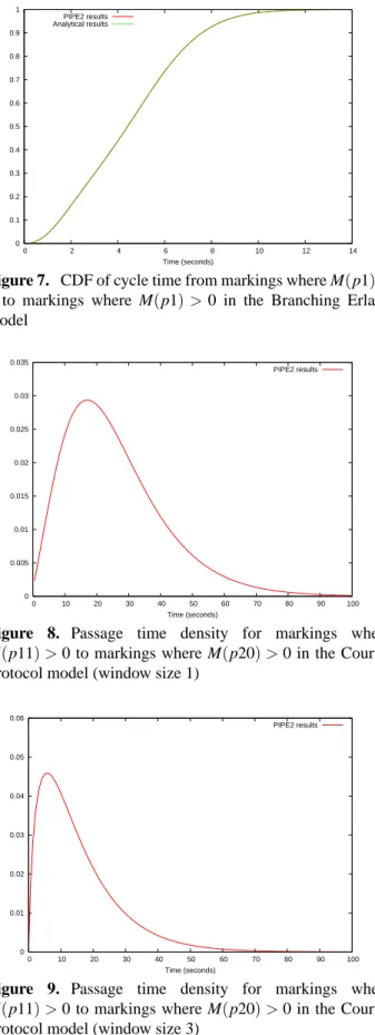
Figures 6 and 7 compare the results produced by PIPE2 and those calculated analytically for the cycle time density and its corresponding CDF function of the Branching Erlang model. Excellent agreement can be seen between the two. These re-sults demonstrate the Response Time Analysis module’s abil-ity to handle cases where the set of source and target states overlap (i.e. to calculate cycle times), as well as bimodal den-sity curves.
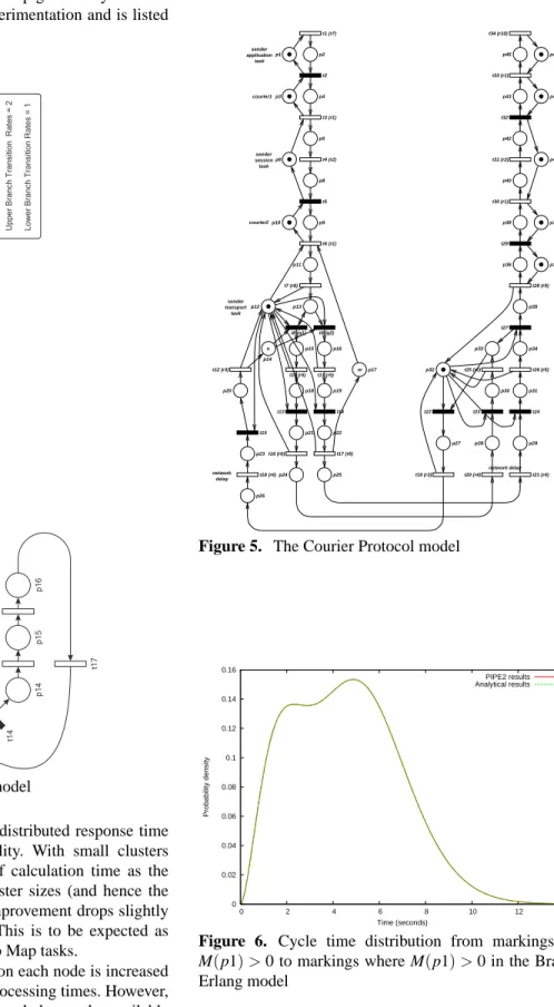
To validate the module for larger models with multiple start and target states we used the Courier Protocol model, first presented in [10] and shown in Figure 5. It models the ISO Application, Session and Transport layers of the Courier sliding-window communication protocol. By increasing the number of tokens on p14, the sliding-window size, we can dramatically increase the state space of the model. We be-gin our validation with this set to one, which results in a state space of 29 010. The module completed this exploration in less than 8 seconds on a single machine. Results for the passage time from the set of markings where M(p11)>0 to those where M(p20)>0 are shown in Figure 8, where
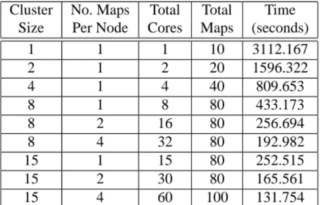
Cluster No. Maps Total Total Time Size Per Node Cores Maps (seconds)
1 1 1 10 3112.167 2 1 2 20 1596.322 4 1 4 40 809.653 8 1 8 80 433.173 8 2 16 80 256.694 8 4 32 80 192.982 15 1 15 80 252.515 15 2 30 80 165.561 15 4 60 100 131.754
Table 1. Laplace transform inversion times for the Courier
Protocol (window size 1) on various cluster sizes
7 320 source markings and 1 860 target markings were iden-tified. They closely match simulation results for this same model that were produced in [6]. It should be noted that our model uses a scaled set of rates that are equal to the original benchmarked rates divided by 5 000. This is necessary as the range in magnitude of the original rates causes problems with the numerical methods used to invert the Laplace transform. The results presented here are the raw results from the PIPE2 module and so must be re-scaled to give the correct timings.
In order to ascertain how the Response Time Analysis module performs with models with larger state spaces we again used the Courier Protocol model, increasing its window size to 3. This results in a state space of 2 162 610 states (in-cluding vanishing states) with 5 469 150 transitions between them. Again, analysing from markings where M(p11)>0 to markings where M(p20)>0, we find there are 439 320 start markings and 273 260 target markings. Results were pro-duced for 50 t-points ranging from 1 to 99 in increments of 2, resulting in a work queue of over 1 800 systems of linear equations, each of rank 2.2 million. State space exploration took 20 minutes, while the Laplace transform inversion took 8 hours 9 minutes on a single node. Generation times for the various other matrices totalled less than 20 seconds.
5.2
Processing Times
Table 1 shows the time taken to perform the Laplace trans-form inversion for the Courier Protocol model (window size 1) for 50 t-points on various cluster sizes. The cluster size column refers to the number of compute nodes assigned to the Hadoop cluster. The second column indicates the number of Map tasks assigned to each node. Hadoop allows multiple Map tasks to be run concurrently on a single node which is of particular benefit with multicore machines as it allows full use to be made of all cores. Where only one Map task was assigned to a node only one core was in use. This was scaled up to 8 and 15 machine clusters until all cores were in use at once. The third column shows the total number of cores being
used simultaneously. The optimum map granularity for each cluster size was found through experimentation and is listed in the fourth column.
Figure 4. The Branching Erlang model
It is clear from Table 1 that the distributed response time calculator offers excellent scalability. With small clusters there is an approximate halving of calculation time as the cluster size is doubled. As the cluster sizes (and hence the number of Map tasks) grow this improvement drops slightly to a factor of approximately 1.8. This is to be expected as there is some overhead in setting up Map tasks.
When the number of cores used on each node is increased we again see a good reduction in processing times. However, we no longer see the calculation time halve as the available cores double. It is likely that this is due to contention for
n courier1 network delay sender application task sender session task sender transport task receiver application task receiver session task receiver transport task m p2 t2 p4 p3 p5 p6 p8 t5 p10 p9 p11 p13 p12 p16 p15 p14 p17 p20 p18 p19 t14 t13 p22 p21 t15 p23 p24 p25 p26 p27 p28 p29 t23 t24 p31 p30 p32 t22 p33 p34 t27 p35 p36 p37 t29 p38 p39 p40 p41 p42 t32 p44 p43 p45 p46 p1 courier3 courier2 courier4 network delay t1 (r7) t3 (r1) t4 (r2) t6 (r1) t7 (r8) t12 (r3) t8 (q1) t9 (q2) t11 (r5) t10 (r5) t18 (r4) t16 (r6) t17 (r6) t34 (r10) t33 (r1) t31 (r2) t30 (r1) t28 (r9) t25 (r5) t26 (r5) t19 (r3) t20 (r4) t21 (r4)
Figure 5. The Courier Protocol model
0 0.02 0.04 0.06 0.08 0.1 0.12 0.14 0.16 0 2 4 6 8 10 12 14 Probability density Time (seconds) PIPE2 results Analytical results
Figure 6. Cycle time distribution from markings where
M(p1)>0 to markings where M(p1)>0 in the Branching
0 0.1 0.2 0.3 0.4 0.5 0.6 0.7 0.8 0.9 1 0 2 4 6 8 10 12 14 Cumulative Probability Time (seconds) PIPE2 results Analytical results
Figure 7. CDF of cycle time from markings where M(p1)>
0 to markings where M(p1)>0 in the Branching Erlang model 0 0.005 0.01 0.015 0.02 0.025 0.03 0.035 0 10 20 30 40 50 60 70 80 90 100 Probability density Time (seconds) PIPE2 results
Figure 8. Passage time density for markings where
M(p11)>0 to markings where M(p20)>0 in the Courier
Protocol model (window size 1)
0 0.01 0.02 0.03 0.04 0.05 0.06 0 10 20 30 40 50 60 70 80 90 100 Probability density Time (seconds) PIPE2 results
Figure 9. Passage time density for markings where
M(p11)>0 to markings where M(p20)>0 in the Courier
Protocol model (window size 3)
shared resources within each node, such as the system bus. Further weight can be added to this argument by comparing the results for jobs run on 8 nodes with jobs run on 15 nodes. A job run on 32 cores spread over 8 nodes takes over 27 sec-onds longer than a job run on only 30 cores, but spread over 15 nodes.
The number of Map tasks for a particular Hadoop job can have a dramatic effect on the time taken to complete the job. While having one Map task per core in the cluster results in the least overhead it can actually result in poor performance. The main reason for this is that Map tasks take different amounts of time to complete, even when each one contains the same number of
L
(s)values to calculate. When running jobs it is not uncommon to see the slowest jobs take over three times as long to complete as the faster ones. It is thought that this is largely due to certainL
(s)values converging fasterthan others. Reducing the granularity, or increasing the num-ber of Map tasks, reduces the length of time each Map task takes, and so reduces the time spent where most of the cluster is idle waiting for the last few Map tasks to complete.
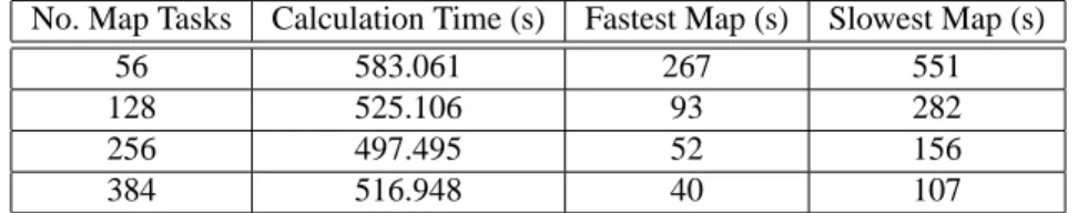
Table 2 shows the time taken to perform the Laplace trans-form inversion for 200 t-points on the Courier Protocol model on a cluster of eight nodes, each running 4 Map Tasks with different numbers of Map Tasks specified. We can see that the optimum granularity for this job is for 256 Map tasks. At this granularity the maximum time to complete a Map task is ap-proximately 150 seconds. This is the maximum time the job will spend waiting for a single Map task to complete when all others have finished. While this time is lower for the 384 Map task job, the benefit is outweighed by the additional overhead of scheduling and configuring an extra 128 Map tasks.
Granularity becomes even more important on heterogenous clusters. The undesirable situation where much of the cluster is idle while the last few Map tasks are executed can be exac-erbated by the scheduler picking slower machines to run these tasks.
6
CONCLUSIONS
We have described the implementation of a Response Time Analysis module for a popular Petri net editor and analyser, PIPE2. This module integrates with Hadoop, an open source Java implementation of the MapReduce distributed program-ming environment to allow the response time analysis of large models using a cluster of commodity computers. While the developers of MapReduce originally intended it to perform relatively simple calculations on massive data sets, we have successfully applied it to a different problem, that of perform-ing complex, computationally intensive calculations on rela-tively smaller data sets. In doing this we have overcome a number of difficulties related to the architecture of Hadoop, whilst retaining the benefits of using a popular open-source project to handle the distribution of processing, such as
ex-No. Map Tasks Calculation Time (s) Fastest Map (s) Slowest Map (s)
56 583.061 267 551
128 525.106 93 282
256 497.495 52 156
384 516.948 40 107
Table 2. Laplace transform inversion times for the Courier Protocol (window size 1) for various granularities
cellent reliability, good fault tolerance and much improved development time.
Models of up to at least 2.2 million states were shown to be easily accommodated using in-core processing. Re-implementing the linear equation solving algorithms as disk-based, rather than in-core, would allow for much larger model sizes.
Results produced by the Response Time Analysis module were validated for smaller models with analytically calcu-lated results and for larger models with simulations. Excellent scalability was shown, with an almost linear improvement in calculation times with increased cluster sizes.
REFERENCES
[1] J. Abate and W. Whitt. The Fourier-series method for inverting transforms of probability distributions.
Queue-ing Systems, 10(1):5–88, 1992.
[2] F. Bause and P.S. Kritzinger. Stochastic Petri Nets: An
Introduction to the Theory. Vieweg Verlag, Wiesbaden,
Germany, 2nd edition, 2002.
[3] P. Bonet, C.M. Llado, R. Puijaner, and W.J. Knottenbelt. PIPE v2.5: A Petri net tool for performance modelling. In Proc. 23rd Latin American Conference on
Informat-ics (CLEI 2007), San Jose, Costa Rica, October 2007.
[4] J.T. Bradley, N.J. Dingle, W.J. Knottenbelt, and H.J. Wilson. Hypergraph-based parallel computation of pas-sage time desnsities in large semi-Markov models. In
Linear Algebra and its Applications: Volume 386, pages
311–334. Elsevier, July 2004.
[5] J. Dean and S. Ghemawat. MapReduce: Simplified data processing on large clusters. In Proceedings of
the OSDI’04: Sixth Symposium on Operating System Design and Implementation, San Francisco, California,
U.S.A., December 2004.
[6] N.J. Dingle, P.G. Harrison, and W.J. Knottenbelt. Re-sponse time densities in Generalised Stochastic Petri net models. In Proceedings of the 3rd ACM Workshop on
Software and Performance (WOSP 2002), pages 46–54,
Rome, Italy, 2002.
[7] T. Kimber, B. Kirby, T. Master, and M. Worthing-ton. Petri nets group project final report. Techni-cal report, Imperial College, London, United Kingdom, March 2007.
[8] W.J. Knottenbelt. Generalised Markovian analysis of timed transition systems. Master’s thesis, University of Cape Town, Cape Town, South Africa, July 1996. [9] W.J. Knottenbelt and P.G. Harrison. Passage time
distri-butions in large Markov chains. In Proceedings of ACM
SIGMETRICS, pages 77–85, Marina Del Rey,
Califor-nia, U.S.A., June 2002.
[10] C.M. Woodside and Y. Li. Performance Petri net analysis of communication protocol software by delay-equivalent aggregation. In Proceeding of the 4th
Inter-national Workshop on Petri nets and Performance Mod-els (PNPM’91), pages 64–73, Melbourne, Australia,