756
|
www.ecolevol.org Ecology and Evolution. 2019;9:756–768.1
|
INTRODUCTION
Occupancy models are an important statistical technique that was developed to make use of detection/nondetection data to infer the probability that a species under investigation occupies a site. When
an occupancy study is undertaken, ns sites are visited a number of times to estimate the occupancy probability (𝝍) and conditional detection probability (p) of a species associated with each site in a region. The method can be viewed as an extension of logistic re‐ gression and allows one to estimate the occupancy probability at Received: 31 August 2018
|
Revised: 14 November 2018|
Accepted: 25 November 2018DOI: 10.1002/ece3.4850
O R I G I N A L R E S E A R C H
Efficient Bayesian analysis of occupancy models with logit link
functions
Allan E. Clark
1,2|
Res Altwegg
1,2This is an open access article under the terms of the Creative Commons Attribution License, which permits use, distribution and reproduction in any medium, provided the original work is properly cited.
© 2019 The Authors. Ecology and Evolution published by John Wiley & Sons Ltd. 1Department of Statistical
Sciences, University of Cape Town, Cape Town, South Africa
2Center for Statistics in Ecology, Environment and Conservation (SEEC), University of Cape Town, Rondebosch, South Africa Correspondence
Allan E. Clark, Department of Statistical Sciences, University of Cape Town, Cape Town, South Africa.
Email: [email protected] Funding information
National Research Foundation of South Africa, Grant/Award Number: 81685 and 99385
Abstract
Occupancy models (Ecology, 2002; 83: 2248) were developed to infer the probability that a species under investigation occupies a site. Bayesian analysis of these models can be undertaken using statistical packages such as WinBUGS, OpenBUGS, JAGS, and more recently Stan, however, since these packages were not developed specifically to fit occupancy models, one often experiences long run times when undertaking an analysis. Bayesian spatial single‐season occupancy models can also be fit using the R package stocc. The approach assumes that the detection and occupancy regression effects are modeled using probit link functions. The use of the logistic link function, however, is algebraically more tractable and allows one to easily interpret the coef‐ ficient effects of an estimated model by using odds ratios, which is not easily done for a probit link function for models that do not include spatial random effects. We de‐ velop a Gibbs sampler to obtain posterior samples from the posterior distribution of the parameters of various occupancy models (nonspatial and spatial) when logit link functions are used to model the regression effects of the detection and occupancy processes. We apply our methods to data extracted from the 2nd Southern African Bird Atlas Project to produce a species distribution map of the Cape weaver (Ploceus capensis) and helmeted guineafowl (Numida meleagris) for South Africa. We found that the Gibbs sampling algorithm developed produces posterior samples that are identical to those obtained when using JAGS and Stan and that in certain cases the posterior chains mix much faster than those obtained when using JAGS, stocc, and
Stan. Our algorithms are implemented in the R package, Rcppocc. The software is freely available and stored on GitHub (https://github.com/AllanClark/Rcppocc). K E Y W O R D S
Bayesian spatial occupancy model, imperfect detection, occupancy model, Rcppocc, restricted spatial regression
sites where none of the species being investigated have been de‐ tected. The model is formulated hierarchically, using Bernoulli ran‐ dom variables to specify the occupancy and detection processes, respectively, which can be modeled using site‐specific and survey‐ specific explanatory variables, respectively (MacKenzie et al., 2002). Johnson, Conn, Hooten, Ray, and Pond (2013) note that occupancy models produce “unbiased inference when occupancy observations at nearby units are conditionally independent given any available covariates” but stress that “spatial autocorrelation may lead to bi‐ ases and overestimated precision” of regression effects. This obser‐ vation has lead to the development of various models to account for spatial autocorrelation in ecological survey data (Aing, Halls, Oken, Dobrow, & Fieberg, 2011; Gardner, Lawler, Ver Hoef, Magoun, & Kellie, 2010; Hoeting, Leecaster, & Bowden, 2000; Hooten, Larsen, & Wikle, 2003) and have extensively been used to guide environ‐ mental monitoring and assessment programs globally.
A number of methods have been used to fit occupancy models to data. These include maximum likelihood (MacKenzie et al., 2002); penalized maximum likelihood (Hutchinson, Valente, Emerson, Betts, & Dietterich, 2015; Moreno & Lele, 2010), Bayesian methods that employ WinBUGS, OpenBUGS, JAGS, or Stan as well as approximate methods such as those developed by Clark, Altwegg, and Ormerod (2016). Recently Dorazio and Rodriguez (2012) and Johnson et al. (2013) developed Gibbs algorithms to obtain posterior samples for the parameters of a nonspatial and spatial single‐season occupancy (SSO) model, respectively. Both approaches assume that detection and occupancy processes are modeled using probit link functions, which enables the use of data augmentation (Tanner & Wong, 1987) to obtain closed form expressions of the conditional posterior distri‐ butions of the parameters of the occupancy model.
Given that the probit and logistic functions are very similar and only differ in respect of the tails of the functions, analysis under‐ taken using either of the functions should produce similar occu‐ pancy and conditional detection probabilities (Dorazio & Rodriguez, 2012). However, the use of the logistic link function is algebraically more tractable and allows one to easily interpret the coefficient ef‐ fects of an estimated model by using odds ratios, which is not easily done for a probit link function. This observation is particularly true for the nonspatial SSO model since no spatial random effects are included in this model; however, when spatial random effects are included in the model, the interpretation of the regression effects can be difficult (Boehm, Reich, & Bandyopadhyay, 2013).
The paper commences with a brief discussion of the link between logistic regression and occupancy models. Thereafter, we discuss the formulation of various popular Bayesian spatial occupancy mod‐ els and develop a Gibbs sampling algorithm for a particular spatial occupancy model when the regression effects of the occupancy and detection processes are modeled using logit link functions. Before concluding, we analyze two detection/nondetection data sets of South African bird species to illustrate the methods developed in the paper. An R package (Rcppocc) has been developed to fit SSO models using Gibbs sampling which can be obtained at: https://github.com/ AllanClark/Rcppocc.
2
|
MATERIAL AND METHODS
2.1
|
Logistic regression and occupancy models
Assume that ns sites are surveyed a number of times and detec‐ tion/nondetection data are collected at all sites. Denote the ob‐ served data as a ragged matrix y=[yij] where yij=1 if the species under investigation has been observed at site i during survey j and yij=0 otherwise. Let the vector z represents the true spe‐ cies occupancy at the sites considered such that zi=1 if the spe‐cies occupies site i and zi=0 if it does not occupy site i. The SSO model can be represented using the following hierarchical model, zi|𝜓i∼Bernoulli(𝜓i), yij|zi,pij∼Bernoulli(zipij) for all sites i=1,…,ns; for all surveys j=1,…,Vi (Royle & Dorazio, 2008). The variable 𝜓i denotes the probability occupancy probability at site i, while pij=Pr(yij=1|zi=1) denotes the conditional probability of de‐
tecting the species during the jth survey of site i given that the species is present at site i. In what follows we assume that the conditional detection and occupancy regression effects (𝜶 and 𝜷) are modeled using logit link functions such that logit(𝜓i)=xTi𝜷 and
logit(pij)=wTij𝜶, where xTi and wTij are row vectors in design matrices,
X (occupancy) and W (detection), respectively (as defined in Clark et al., 2016).
The joint posterior distribution of the parameters of the model is
where 𝜋(𝜶) and 𝜋(𝜷) are the prior distributions of 𝜶 and 𝜷, respec‐
tively. A directed acyclic graph of the above problem is displayed in Figure 1 below.
A Gibbs sampling algorithm for the parameters of this model re‐ quires sampling from [𝜷|z], [𝜶|z,y], and [zi=1|𝜶,𝜷,y] for all sites where
[z,𝜶,𝜷|y]∝𝜋(𝜶)𝜋(𝜷) (n s ∏ i=1 𝜓zi i (1−𝜓i)1−zi ) ∏ i ∏ j {i:zi=1} pyij ij(1−pij)1−yij
F I G U R E 1 A directed acyclic graph illustrating the
dependencies between the parameters and observed data for an SSO model. Shaded nodes represents observed data while all latent parameters are represented using unshaded nodes. Deterministic relationships are represented using double arrows while all stochastic relationships are represented using a single arrow
yi,j pi,j zi α ψi β xi wi,j j= 1, . . . , Vi i= 1, . . . , ns
the species has not been observed. The first two conditional distri‐ butions have the following form,
Notice that Equations 1 and 2 are of the same form as the pos‐ terior distributions of the regression effects of a logistic regression model and therefore we adapt a Gibbs sampling scheme for logis‐ tic regression models to address the problem of obtaining posterior samples for the parameters of an occupancy model.
In a logistic regression context, Polson, Scott, and Windle (2013) show that posterior samples of the regression effects can be ob‐ tained by sampling from the conditional distributions of Pólya‐ Gamma random variables and multivariate Gaussian distributions in turn. Their method is similar to that of Albert and Chib (1993) who developed a Gibbs algorithm to undertake probit regression, the only difference being that the sampling from truncated Gaussian distribu‐ tions is replaced by sampling from Pólya‐Gamma distributions. The sampling methods developed by Polson et al. (2013) are exact since their Pólya‐Gamma sampling method is uniformly ergodic and con‐ verges to the correct posterior distribution (Choi, & Hobert, 2013).
For the SSO model, the conditional posterior distributions of 𝜷|𝝎𝜷,y are derived by introducing Pólya‐Gamma latent variables,
𝝎𝜷, and noting that the contribution of the i^
{th} observation to a Bernoulli likelihood can be re‐expressed as
where 𝜅i=zi−0.5 and p(𝜔i,𝜷|1,0) is the probability density function
of a Pólya‐Gamma distribution with parameters 1 and 0 (Polson et al., 2013). The conditional posterior distribution of 𝜶 is derived by using the same manipulation of the Bernoulli likelihood.
In the Supporting information (Appendix S1), we discuss the ex‐ isting Gibbs algorithms used for undertaking logistic regression and demonstrate the use of the Pólya‐Gamma (PG) method by developing two Gibbs sampling algorithms for the parameters of SSO models. In Table 1, we summarize the Gibbs algorithms for an SSO model when using the PG method but provide the details regarding the algorithm in the Supporting Information (Appendix S2 and Appendix S3). We use the notation “a∼PG(b,c)” to indicate that the random variable a is a Pólya‐Gamma random variable with parameters b and c. Take note that the algorithm is identical to that developed by Dorazio and Rodriguez (2012) except that the sampling from truncated Gaussian distributions is replaced by sampling from Pólya‐Gamma distributions.
2.2
|
Bayesian spatial SSO models
Spatial generalized linear mixed models (SGLMM) are an exten‐ sion of the general linear model (Nelder & Wedderburn, 1972) that
allows the link function of the expected value of the random variable under investigation to be modeled as a function of a spatial random variable/s. The formulation was first developed by Besag, York, and Mollié (1991) and has been extensively used in areas such as agri‐ culture (Besag & Higdon, 1999), biostatistics (Gelfand & Vounatsou, 2003; Waller & Gotway, 2004), ecology (Lichstein, Simons, Shriner, & Franzreb, 2002) and species distribution modelling (Drouilly, Clark, & O'Riain, 2018; Gelfand et al., 2005; Hooten et al., 2003; Latimer, Wu, Gelfand, & Silander, 2006).
The paper by Gelfand et al. (2005) lead to the development of the R package hSDM (Vieilledent et al., 2014) in which the hSDM.siteocc.iCAR function can be used to fit a particular spa‐ tial occupancy model to detection/nondetection data. A region under investigation is subdivided into ns grid cells each which are surveyed a number of occasions. The model is formulated using Bernoulli latent random variables z=(z1,…,zns)
T. Formally, zi|𝜓i∼Bernoulli(𝜓i) with logit(𝜓i)=xTi𝜷+𝜌i, for alli=1,…,n, where 𝝆=(𝜌1,…,𝜌ns)
T is a multivariate Gaussian random vector with mean 0 and correlation matrix defined using the neighborhood structure of the grid cells. The observation process is specified as in the non‐ spatial model. The documentation of the function indicates that pos‐ terior samples of the parameters of the model are obtained using the C programming language and utilizes an adaptive Metropolis al‐ gorithm (Metropolis, Rosenbluth, Rosenbluth, Teller, & Teller, 1953; Robert & Casella, 2013).
Johnson et al. (2013) develop two spatial occupancy models. They assume that probit link functions are used to model both the occu‐ pancy and detection processes and thereby rely on data augmentation to develop a Gibbs sampling algorithm to sample from the posterior distribution of the parameter of the models. For the probit case, the occupancy probability of a particular grid cell (for the standard occu‐ pancy model) is calculated as Φ(xT
i𝜷)=Pr(zi=1). In a Bayesian con‐ text, such a probit model is formulated by defining a latent Gaussian (1) [𝜷�z]∝𝜋(𝜷) ns ∏ i=1 𝜓zi i (1−𝜓i)1−ziand (1) [𝜶�z,y]∝𝜋(𝜶)∏ i ∏ j {i:zi=1} pyij ij(1−pij)1−yij. (2) 𝜓zi i(1−𝜓i)1−zi= exp(xT i𝜷) zi 1+exp(xT i𝜷) =exp (𝜅ixT i𝜷)∫exp ( −𝜔i,𝜷 2(x T i𝜷)2 ) p(𝜔i,𝜷|1,0)d𝜔i,𝜷 ,
TA B L E 1 The Gibbs algorithm for undertaking a SSO model using the “PG” method (See the Supporting Information (Appendix S3) for the details pertaining to the parameter matrices of the conditional posterior distributions.)
random variable, z̃i with mean 0 and variance equal to 1 such that Pr(zi=1)=Pr(̃zs>0). In the first of their models, they allow ̃zs to be spatially correlated such that ̃zi=xT
i𝜷+𝜂i+𝜖i. 𝜼=(𝜂1,…,𝜂ns)
T is de‐ fined as 𝝆 above while 𝜖i∼(0,1), for alli=1,…,ns.
Often the spatial random effects and fixed effects of a model are collinear when spatially varying covariates are included as fixed effects (Hanks, Schliep, Hooten, & Hoeting, 2015; Hodges & Reich, 2010; Hughes & Haran, 2013; Reich, Hodges, & Zadnik, 2006). The suggested solution to this problem was to include spatial random effects in the model specification that are orthogonal to the fixed effects and is known as restricted spatial regression (RSR). The sec‐ ond spatial model developed by Johnson et al. (2013) uses this method and redefines z̃i as z̃i=xT
i𝜷+k
T
i𝜽+𝜖i, where k T
i is a row vector of the design matrix K. The spatial random effects are mod‐ eled as
Q is a n×n ICAR precision matrix (Besag & Kooperberg, 1995) obtained using surveyed and unsurveyed locations, 𝜏 is a spatial pre‐
cision parameter and i1 and i2 are known constants. Kelsall and Wakefield (1999) have suggested setting these parameters to 0.5 and 0.005, respectively, such that the prior mean of 𝜏 is 1,000. The
matrix K consists of the first r (r ≪ n) eigenvectors of 𝛀=nRAR∕1TA1 where R=In−X
( XTX
)−1
XT and A is an association matrix with (ij)th entry Aij=1 if sites i and j are neighbours and zero otherwise.
In our formulation of the spatial occupancy model, we model the occupancy probabilities at all grid cells as
where K and 𝜽 are defined above. We make use of Pólya‐Gamma random variables to obtain the conditional distributions of the pa‐ rameters of the above spatial occupancy model. The conditional distributions are very similar to those obtained for the SSO model although here we require the conditional posterior distribution of additional parameters (𝜽 and 𝜏). A directed acyclic graph of the
spatial SSO model is displayed in Figure 2 below while in Table 2, we summarize the Gibbs algorithms for a spatial SSO model which employs Equation 3 when using the PG method. The details re‐ garding the algorithm can be found in the Supporting information (Appendix S4).
2.3
|
Applications
To demonstrate our methods, we used detection/nondetection data extracted from the 2nd Southern African Bird Atlas Project (SABAP2) database to produce a species distribution map of the Cape weaver (Ploceus capensis) and helmeted guineafowl (Numida meleagris) for South Africa. SABAP2 divides Southern Africa into a continuous grid of 5′ × 5′ and relies on citizen scientists to collect checklists of bird species for each grid cell. Birders are requested
to spend at least 2 hr on each checklist in which they undertake in‐ tense birding and record all species they observe and the order in which they are observed. For this analysis, we aggregated the data to quarter‐degree grid cells. We used data that span South Africa and contained a minimum of three and a maximum of fifty surveys during 2016 (January–December) in the analysis. Covariate information at unsurveyed locations was included in the analyses to obtain occu‐ pancy estimates that span South Africa. All covariates were centered and standardized. 𝜽|𝜏∼ ( 0r, 1 𝜏 ( KTQK )−1) =(0r, 1 𝜏M ) , 𝜏∼(i1,i2) and𝝐∼(0n,In). (3) logit(𝜓i)=xTi𝜷+k T i𝜽,
F I G U R E 2 A directed acyclic graph illustrating the
dependencies between the parameters and observed data for a spatial SSO model. Shaded nodes represents observed data while all latent parameters are represented using unshaded nodes. Deterministic relationships are represented using double arrows while all stochastic relationships are represented using a single arrow yi,j pi,j zi α ψi β θ τ xi wi,j j= 1, . . . , Vi i= 1, . . . , ns
TA B L E 2 The Gibbs algorithm for undertaking a spatial SSO model (See the Supporting Information (Appendix S4) for the details pertaining to the parameter matrices of some of the conditional posterior distributions.)
In our analysis, we fitted a nonspatial and spatial SSO model with one detection covariate and two occupancy covariates. The detection covariate used was the number of species observed by the birder (denoted as nspp), while the occupancy covariates were functions of seven climate variables. It is assumed that the more spe‐ cies the birder observes while birding, the more likely they are to observe the particular species being analyzed such that a positive detection regression effect is expected. The aim of the analysis is not to obtain the best occupancy model for the particular data sets but rather to highlight the use of the developed Gibbs sampling al‐ gorithm for fitting RSR occupancy models to the data using different software programs and different sampling methods. We specifically consider the Gibbs sampling algorithm by Johnson et al. (2013) (pro‐ bit link functions), our Gibbs algorithm (logit link functions), JAGS, and Stan (which uses a no‐U‐turn Hamiltonian Monte Carlo sampler (Hoffman & Gelman, 2014) to sample from the parameters of a pos‐ terior distribution).
The climate variables (Figure S5 in the Supporting Information Appendix S6) all form part of a data set used by Huntley et al. (2006) to model bird distributions in Southern Africa. The variables included two measures of annual temperature that related to thermal sums above 0 and 5 degree centigrade; two measures related to the mean temperature of the coldest and warmest month, respectively; the ratio of potential to realized evapotranspiration as well as two mea‐ sures that relates to the intensity of the dry and wet season, respec‐ tively. The climate variables are highly correlated with two of the variables having variance inflation factors in excess of 3,000 (Tables S2 and S3 in the Supporting Information Appendix S5). Because of this fact, it was decided to extract two principal components from the design matrix that consisted of the centered and standardized climate variables. These principal components explain 90% of the variation in the design matrix (Table S4 in the Supporting Information Appendix S5) and can tentatively be interpreted as a temperature re‐ lated factor and a climate intensity factor, respectively.
We follow Hughes and Haran (2013) and retain 10% of the eigen‐ values (𝜆ii=1,…,n) of 𝛀. In a similar context, Johnson et al. (2013) suggest selecting a RSR model with 𝜆i≥0.5 which suggests includ‐
ing at most 237 eigenvectors into the spatial portion of the model.
Experimentation with different values of r between 150 and 230 demonstrated no significant difference to the results we report here.
The following prior distributions were used for the parameters of the spatial SSO model: 𝜶∼(0,1000I2), 𝜷∼(0,1000I3), and
𝜏∼(0.5,0.005). The prior specification for 𝜏 places more weight on
large values of 𝜏 indicating that very little prior weight is placed on
the spatial random effects of the model. Broms (2013) performed a simulation study and found that the RSR model results are not sensitive to the prior specification of 𝜏 and thus we have not done
any analysis to test the sensitivity of our results to the prior speci‐ fication of 𝜏. All MCMC sampling was undertaken using the R pack‐
ages, stocc, jagsUI (Kellner, 2014) in combination with JAGS 4.2.0 (Plummer, 2003), rstan in combination with Stan 2.17.3 as well as the authors’ code.1 All calculations were performed on a Windows 10 Pro desktop computer which had an Intel(R) Core(TM) i7‐6900 processor with 64 GB of RAM. One chain of 70,000 iterations was run. The first 20,000 samples were discarded as burn‐in samples, while the remaining samples were retained. Experimentation and an examination of the Geweke convergence diagnostic statistics (Geweke, 1992) and trace plots obtained by running three parallel chains using Rcppocc displayed that the MCMC chains converged using these numbers of iterations. The posterior samples were not thinned (Link & Eaton, 2012).
3
|
RESULTS
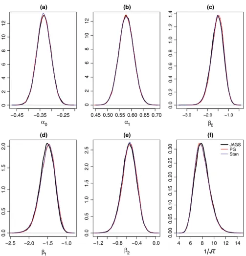
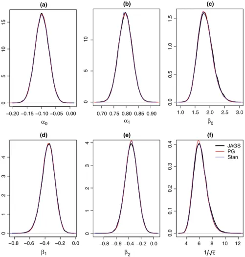
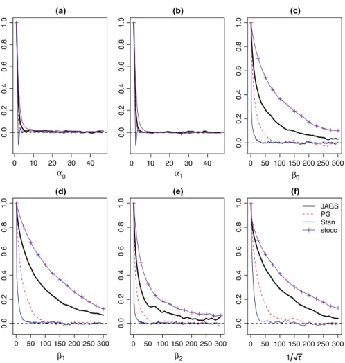
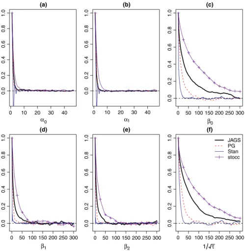
From the analysis of both data sets, we observe that the Gibbs algo‐ rithm developed for the spatial occupancy model produces identical posterior distributions to those obtained when using JAGS and Stan (Figures A1 and A2 in Appendix 1). In both data sets, the posterior samples of the detection regression effects exhibit good mixing where the lagged sample autocorrelations of the posterior samples approach zero within 5 lags. The posterior samples of the occupancy regression effects as well as the precision of the spatial random ef‐ fect (𝜏) exhibit slower mixing when using stocc, JAGS, and Rcppocc
(denoted as “PG” in Figures A3 and A4 in Appendix 2), while Stan produced a posterior chain that mixed well. We observe that stocc
TA B L E 3 Posterior run times for the Bayesian spatial occupancy models as well as the ESR (per minute) for 𝜶, 𝜷, and 𝜏
Species Method Time (min) 𝛼0 𝛼1 𝛽0 𝛽1 𝛽2 𝜏
Cape weaver stocc (RSR) 27.00 552.71 725.59 12.03 7.83 22.37 11.35
stocc (ICAR) 136.76 104.41 142.57 0.25 0.10 0.15 0.14
JAGS 243.55 102.62 131.42 2.69 1.71 5.09 1.97
Stan 187.06 275.75 331.44 53.48 34.42 83.74 19.35
Rcppocc 19.88 1682.15 1804.42 85.32 53.40 141.82 116.19
Helmeted Guinea
fowl stoccstocc (RSR) (ICAR) 27.08165.23 65.92619.72 563.2497.15 11.630.04 0.1643.61 0.0948.34 15.610.05
JAGS 254.49 97.86 125.35 3.08 10.84 12.06 2.66
Stan 150.55 595.77 617.84 49.21 186.23 286.92 24.44
produced posterior samples for 𝜶, 𝜷, and 𝜏 that had the largest levels
of autocorrelation among all of the methods considered (when fit‐ ting the RSR model).
Table 3 tabulates the run times (in minutes) and effective sam‐ pling rate (ESR2 = the effective sample size per unit run time) of α, β, and τ for each of the sampling algorithms used to analyze the two data sets. For completeness sake, we also include the statis‐ tics related to the ICAR model when using stocc. We observe that stocc and Rcppocc had faster run times than JAGS and Stan. Rcppocc had the fastest running times and completed the 70,000 MCMC iterations approximately 12 times faster than JAGS and between 7 and 10 times faster than Stan. Rcppocc has the largest ESR of all of the algorithms considered and produced ESR values which ranged between 1.5 and 6 times larger than those obtained by Stan; 3–11 times larger than those obtained by stocc and 11–60 times larger than those obtained by JAGS. The ICAR models took approximately 8 times longer to run than the RSR model when using stocc and resulted in significantly larger levels of autocorrelation within the 𝜶, 𝜷, and 𝜏 chains.
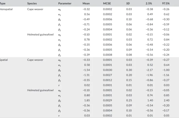
The posterior summaries for some of the parameters of the nonspatial and spatial model are displayed in Table 4. The fixed re‐ gression effects of all of the parameters (for both data sets) were statistically different from zero since none of the 95% highest
density credibility interval of the parameters contained zero. In all cases, the regression effect for nspp was positive (as expected), while the regression effects of the occupancy effects were neg‐ ative. The detection regression effects for both model types (for the respective species) were identical. The regression effects for the occupancy process for the Cape weaver were significantly dif‐ ferent for the two model types, while the same regression effects for the helmeted guineafowl were identical for both model types (except for the intercept). The posterior distribution of the spatial standard deviation parameter (𝜎=1∕√𝜏) indicates that the spatial
process does significantly contribute to the variability of the occu‐ pancy process across South Africa. The 95% posterior highest den‐ sity credibility interval for 𝜎 is [5.56, 10.59] and [4.26, 8.42] for the
Cape weaver and the helmeted guineafowl data sets, respectively. Figure 3a,c displays the estimated occupancy probabilities (Pr (zi=1|.)) across South Africa estimated using Rcppocc for the Cape
weaver and helmeted guineafowl data set, respectively. The figures illus‐ trate that there is a high probability that the Cape weaver occupies coastal regions throughout South Africa and low occupancy probability (close to zero) in the interior areas of South Africa. In contrast, the helmeted guin‐ eafowl has very high occupancy probabilities in most regions of South Africa except for the North West regions of South Africa. Figure 3b,d displays the difference between the estimated occupancy probabilities
TA B L E 4 Posterior summaries of the parameters of the Bayesian nonspatial and spatial occupancy models (posterior mean, Monte Carlo standard error, standard deviation, 2.5% and 97.5% quantiles)
Type Species Parameter Mean MCSE SD 2.5% 97.5%
Nonspatial Cape weaver 𝛼0 −0.32 0.0002 0.03 −0.38 −0.26
𝛼1 0.56 0.0002 0.03 0.49 0.62 𝛽0 −0.49 0.0006 0.10 −0.68 −0.30 𝛽1 −0.71 0.0005 0.06 −0.84 −0.59 𝛽2 −0.24 0.0004 0.06 −0.36 −0.12 Helmeted guineafowl 𝛼0 −0.10 0.0001 0.02 −0.15 −0.06 𝛼1 0.78 0.0002 0.03 0.72 0.84 𝛽0 −0.35 0.0006 0.06 −0.48 −0.22 𝛽1 −0.36 0.0005 0.09 −0.54 −0.20 𝛽2 −0.39 0.0008 0.08 −0.56 −0.24
Spatial Cape weaver 𝛼0 −0.33 0.0001 0.03 −0.39 −0.27
𝛼1 0.58 0.0001 0.03 0.52 0.64 𝛽0 −1.54 0.0030 0.30 −2.17 −1.00 𝛽1 −1.51 0.0027 0.20 −1.96 −1.16 𝛽2 −0.55 0.0012 0.15 −0.86 −0.27 𝜏 0.02 0.0001 0.01 0.01 0.03 Helmeted guineafowl 𝛼0 −0.10 0.0001 0.02 −0.15 −0.05 𝛼1 0.80 0.0001 0.03 0.74 0.85 𝛽0 1.85 0.0029 0.25 1.40 2.40 𝛽1 −0.36 0.0005 0.09 −0.54 −0.20 𝛽2 −0.36 0.0004 0.10 −0.56 −0.17 𝜏 0.03 0.0002 0.01 0.01 0.05
obtained when using Rcppocc and stocc, respectively (“Rcppocc‐stocc”). The figures illustrate that we obtain similar estimates of the mean oc‐ cupancy probabilities when using either estimation method with small discrepancies at the majority of the grid cells across South Africa.
4
|
DISCUSSION AND CONCLUSIONS
Through several studies, Bayesian methods have been developed to undertake occupancy models. They, however, either use probit
link functions to model the detection and occupancy processes of the model; use general Bayesian analysis software such as JAGS, WinBUGS, OpenBUGS, or Stan to undertake their analysis or make use of the Metropolis–Hastings algorithm to sample from the pa‐ rameters of the model. We develop a Gibbs sampling algorithm to obtain posterior samples of the parameters of a restricted spa‐ tial regression (RSR) occupancy model and demonstrate that the method has a larger expected sampling rate (ESR) and faster run times when compared to previous Bayesian methods used in the literature to date.
F I G U R E 3 Estimated occupancy probability for the Cape weaver and helmeted guineafowl estimated using Rcppocc (a and c). The difference between the estimated occupancy probabilities obtained when using Rcppocc and stocc for the Cape weaver and helmeted guineafowl, respectively (b and d). The grid cells where the species have been detected at least once are displayed in (b) and (d)
(a)
(c) (d)
Similar to Broms, Johnson, Altwegg, and Conquest (2014) and Johnson et al. (2013), we show that the ICAR model produced poste‐ rior samples with significantly larger autocorrelations than the RSR model when using stocc. As an example, the autocorrelations of the occupancy regression effects as well as the spatial precision param‐ eter (of both data sets) had autocorrelations in excess of 0.7 at lag 500 indicating that the posterior chain of the model mixed poorly for those parameters of the ICAR model. Additionally, the run times of the ICAR model were approximately 5 times longer than the run times of the RSR model and thus we do not recommend its use when fitting a spatial occupancy model.
Based on the two data sets, we observed that the new algo‐ rithm not only ran faster (approximately 35%) than the Gibbs sam‐ pler implemented in stocc, it also generated expected sample size (ESS) statistics between 2 and 6 times larger than those obtained using stocc. The main reason for the time difference is that stocc has been coded using R, while Rcppocc uses Rcpp and RcppArmadillo to undertake all matrix computations. Stan uses compiled C++ code to implement the no‐U‐turn Hamiltonian Monte Carlo algorithm and generated ESS statistics between 2 and 7 times larger than those obtained using Rcppocc. In many applications, Stan has been shown to be much faster than JAGS although at present Stan has run times that are approximately 7–10 times slower than Rcppocc when fitting spatial occupancy models. The opportunity thus exists to develop suitable Stan (or NIMBLE) code that can fit spatial occupancy models in a shorter period of time.
ACKNOWLEDGMENTS
This research was partially supported by two South African National Research Foundation grants, namely, 99385 (Clark) and 81685 (Altwegg). The financial assistance of the NRF toward this research is hereby acknowledged. Opinions expressed and conclusions arrived at, are those of the author and are not necessarily to be attributed to the NRF. Allan Clark would also like to acknowledge the help of Andrew D. Crosby, a Postdoctoral Fellow at the Boreal Avian Modelling Project, Department of Biological Sciences, University of Alberta. He shared code (with Allan Clark) on how to fit the single‐season occupancy model using Stan via email correspondence. The authors would also like to thank Prof Linda Haines (University of Cape Town) for reading the initial manuscript and providing helpful comments.
CONFLIC T OF INTEREST
The authors have no conflict of interests to declare.
AUTHOR CONTRIBUTION
Below, Allan Ernest Clark is denoted as “AEC”, while Res Altwegg is denoted as “RA”. AEC and RA conceived and designed the paper. AEC analyzed the data. AEC wrote and, AEC and RA reviewed the paper. AEC designed and coded the software used in the analysis. AEC wrote computer code used to perform all analysis.
Notes
1An R package has been developed to fit these models using MCMC.
All code can be obtained from https://github.com/AllanClark/Rcppocc. Appendix S7 in the Supporting Information includes a worked example
explaining how to run RSR models using stocc, Stan, and Rcppocc.
2ESR = the effective sample size per unit run time. The effec‐
tive sample size for the ith parameter in the model is defined as
ESSi=M∕1+2∑kj=1𝜌i(j), where M is the number of retained samples,
and 𝜌i(j) is the jth lagged autocorrelation of parameter i (Holmes &
Held, 2006). We use the coda package (Plummer, Best, Cowles, &
Vines, 2006) to estimate ESSi.
ORCID
Allan E. Clark https://orcid.org/0000-0003-3472-0797
REFERENCES
Aing, C., Halls, S., Oken, K., Dobrow, R., & Fieberg, J. (2011). A bayesian hierarchical occupancy model for track surveys conducted in a series
of linear, spatially correlated, sites. Journal of Applied Ecology, 48(6),
1508–1517. https://doi.org/10.1111/j.1365-2664.2011.02037.x Albert, J. H., & Chib, S. (1993). Bayesian analysis of binary and polychot‐
omous response data. Journal of the American Statistical Association,
88(422), 669–679. https://doi.org/10.1080/01621459.1993.104763 21
Besag, J., & Higdon, D. (1999). Bayesian analysis of agricul‐
tural field experiments. Journal of the Royal Statistical Society:
Series B (Statistical Methodology), 61(4), 691–746. https://doi. org/10.1111/1467-9868.00201
Besag, J., & Kooperberg, C. (1995). On conditional and intrinsic autore‐
gressions. Biometrika, 82(4), 733–746.
Besag, J., York, J., & Mollié, A. (1991). Bayesian image restoration, with
two applications in spatial statistics. Annals of the Institute of Statistical
Mathematics, 43(1), 1–20. https://doi.org/10.1007/BF00116466 Boehm, L., Reich, B. J., & Bandyopadhyay, D. (2013). Bridging condi‐
tional and marginal inference for spatially referenced binary data.
Biometrics, 69(2), 545–554. https://doi.org/10.1111/biom.12027 Broms, K. M. (2013). Using Presence‐Absence Data on Areal Units to
Model the Ranges and Range Shifts of Select South African Bird Species. PhD thesis.
Broms, K. M., Johnson, D. S., Altwegg, R., & Conquest, L. L. (2014). Spatial occupancy models applied to atlas data show Southern Ground
Hornbills strongly depend on protected areas. Ecological Applications,
24(2), 363–374. https://doi.org/10.1890/12-2151.1
Choi, H. M., & Hobert, J. P. (2013). The polya‐gamma gibbs sampler for
bayesian logistic regression is uniformly ergodic. Electronic Journal of
Statistics, 7, 2054–2064.https://doi.org/10.1214/13-EJS837 Clark, A. E., Altwegg, R., & Ormerod, J. T. (2016). A variational Bayes
approach to the analysis of occupancy models. PLoS ONE, 11(2),
e0148966. https://doi.org/10.1371/journal.pone.0148966
Dorazio, R. M., & Rodriguez, D. T. (2012). A Gibbs sampler for Bayesian
analysis of site‐occupancy data. Methods in Ecology and Evolution, 3(6),
1093–1098. https://doi.org/10.1111/j.2041-210X.2012.00237.x Drouilly, M., Clark, A., & O'Riain, M. J. (2018). Multi‐species oc‐
cupancy modelling of mammal and ground bird communities in rangeland in the karoo: A case for dryland systems globally.
Biological Conservation, 224, 16–25. https://doi.org/10.1016/j. biocon.2018.05.013
Gardner, C. L., Lawler, J. P., Ver Hoef, J. M., Magoun, A. J., & Kellie, K. A. (2010). Coarse‐scale distribution surveys and occur‐ rence probability modeling for wolverine in interior Alaska.
Journal of Wildlife Management, 74(8), 1894–1903. https://doi. org/10.2193/2009‐386
Gelfand, A. E., Schmidt, A. M., Wu, S., Silander, J. A., Latimer, A., & Rebelo, A. G. (2005). Modelling species diversity through species
level hierarchical modelling. Journal of the Royal Statistical Society:
Series C (Applied Statistics), 54(1), 1–20.
Gelfand, A. E., & Vounatsou, P. (2003). Proper multivariate conditional
autoregressive models for spatial data analysis. Biostatistics, 4(1),
11–15. https://doi.org/10.1093/biostatistics/4.1.11
Geweke, J. (1992). Evaluating the accuracy of sampling‐based approaches
to the calculations of posterior moments. Bayesian Statistics, 4,
641–649.
Hanks, E. M., Schliep, E. M., Hooten, M. B., & Hoeting, J. A. (2015). Restricted spatial regression in practice: geostatistical mod‐ els, confounding, and robustness under model misspecification.
Environmetrics, 26(4), 243–254. https://doi.org/10.1002/env.2331 Hodges, J. S., & Reich, B. J. (2010). Adding spatially‐correlated errors can
mess up the fixed effect you love. The American Statistician, 64(4),
325–334. https://doi.org/10.1198/tast.2010.10052
Hoeting, J. A., Leecaster, M., & Bowden, D. (2000). An improved model
for spatially correlated binary responses. Journal of Agricultural,
Biological, and Environmental Statistics, 5(1), 102–114. https://doi. org/10.2307/1400634
Hoffman, M. D., & Gelman, A. (2014). The No-U-turn sampler: Adaptively
setting path lengths in Hamiltonian Monte Carlo. Journal of Machine
Learning Research, 15(1), 1593–1623.
Holmes, C. C., & Held, L. (2006). Bayesian auxiliary variable models for
binary and multinomial regression. Bayesian Analysis, 1(1), 145–168.
https://doi.org/10.1214/06-BA105
Hooten, M. B., Larsen, D. R., & Wikle, C. K. (2003). Predicting the spa‐ tial distribution of ground flora on large domains using a hierarchi‐
cal bayesian model. Landscape Ecology, 18(5), 487–502. https://doi.
org/10.1023/A:1026001008598
Hughes, J., & Haran, M. (2013). Dimension reduction and alleviation of
confounding for spatial generalized linear mixed models. Journal of
the Royal Statistical Society: Series B (Statistical Methodology), 75(1), 139–159. https://doi.org/10.1111/j.1467-9868.2012.01041.x Huntley, B., Collingham, Y. C., Green, R. E., Hilton, G. M., Rahbek, C.,
& Willis, S. G. (2006). Potential impacts of climatic change upon
geographical distributions of birds. Ibis, 148(s1), 8–28. https://doi.
org/10.1111/j.1474-919X.2006.00523.x
Hutchinson, R. A., Valente, J. J., Emerson, S. C., Betts, M. G., & Dietterich, T. G. (2015). Penalized likelihood methods improve parameter esti‐
mates in occupancy models. Methods in Ecology and Evolution, 6(8),
949–959. https://doi.org/10.1111/2041-210X.12368
Johnson, D. S., Conn, P. B., Hooten, M. B., Ray, J. C., & Pond, B. A. (2013).
Spatial occupancy models for large data sets. Ecology, 94(4), 801–
808. https://doi.org/10.1890/12-0564.1
Kellner, K. (2014). jagsui: Run JAGS (specifically, libjags) from R: an alter‐
native user interface for rjags. R package version, 1.
Kelsall, J., & Wakefield, J. (1999). Contribution to: “Bayesian models for spatially correlated disease and exposure data”. In N. G. Best, L. A.
Waller, A. Thomas, E. M. Conlon & R. Arnold (Eds.), Bayesian Statistics
6, Proceedings of the Sixth Valencia International Meeting, (Vol.6 pp. 51). Oxford, UK: Oxford University Press.
Latimer, A. M., Wu, S., Gelfand, A. E., & Silander, J. A. (2006). Building
statistical models to analyze species distributions. Ecological
Applications, 16(1), 33–50. https://doi.org/10.1890/04-0609 Lichstein, J. W., Simons, T. R., Shriner, S. A., & Franzreb, K. E.
(2002). Spatial autocorrelation and autoregressive models in
ecology. Ecological Monographs, 72(3), 445–463. https://doi.
org/10.1890/0012-9615(2002)072[0445:SAAAMI]2.0.CO;2
Link, W. A., & Eaton, M. J. (2012). On thinning of chains in MCMC.
Methods in Ecology and Evolution, 3(1), 112–115. https://doi. org/10.1111/j.2041-210X.2011.00131.x
MacKenzie, D. I., Nichols, J. D., Lachman, G. B., Droege, S., Andrew Royle, J., & Langtimm, C. A. (2002). Estimating site occupancy
rates when detection probabilities are less than one. Ecology,
83(8), 2248–2255. https://doi.org/10.1890/0012-9658(2002)083 [2248:ESORWD]2.0.CO;2
Metropolis, N., Rosenbluth, A. W., Rosenbluth, M. N., Teller, A. H., & Teller, E. (1953). Equation of state calculations by fast computing ma‐
chines. The Journal of Chemical Physics, 21(6), 1087–1092. https://doi.
org/10.1063/1.1699114
Moreno, M., & Lele, S. R. (2010). Improved estimation of site occupancy
using penalized likelihood. Ecology, 91(2), 341–346. https://doi.
org/10.1890/09‐1073.1
Nelder, J., & Wedderburn, R. (1972). Generalized linear model. Journal of the Royal Statistical Society, 135(3), 370–384. https://doi. org/10.2307/2344614
Plummer, M. (2003). JAGS: A program for analysis of Bayesian graphical
models using Gibbs sampling. In Proceedings of the 3rd international
workshop on distributed statistical computing, (Vol. 124, pp. 125). Wien, Austria: Technische Universit at Wien.
Plummer, M., Best, N., Cowles, K., & Vines, K. (2006). CODA: Convergence
diagnosis and output analysis for MCMC. R News, 6(1), 7–11.
Polson, N. G., Scott, J. G., & Windle, J. (2013). Bayesian inference for
logistic models using Pólya‐Gamma latent variables. Journal of the
American Statistical Association, 108(504), 1339–1349. https://doi.or g/10.1080/01621459.2013.829001
Reich, B. J., Hodges, J. S., & Zadnik, V. (2006). Effects of resid‐ ual smoothing on the posterior of the fixed effects in disease‐
mapping models. Biometrics, 62(4), 1197–1206. https://doi.
org/10.1111/j.1541-0420.2006.00617.x
Robert, C., & Casella, G. (2013). Monte Carlo statistical methods. New
York: Springer-Verlag.
Royle, J. A., & Dorazio, R. M. (2008). Hierarchical modeling and inference
in ecology: The analysis of data from populations, metapopulations and communities. San Diego, CA: Academic Press.
Tanner, M. A., & Wong, W. H. (1987). The calculation of posterior dis‐
tributions by data augmentation. Journal of the American Statistical
Association, 82(398), 528–540. https://doi.org/10.1080/01621459.1 987.10478458
Vieilledent, G., Merow, C., Guélat, J., Latimer, A., Kéry, M., Gelfand, A., … Silander, J. Jr (2014). hsdm: Hierarchical bayesian species distribution models. R package version 1.4.
Waller, L. A., & Gotway, C. A. (2004). Applied spatial statistics for public health data, Vol. 368. New York: Wiley.
SUPPORTING INFORMATION
Additional supporting information may be found online in the Supporting Information section at the end of the article.
How to cite this article: Clark AE, Altwegg R. Efficient Bayesian analysis of occupancy models with logit link functions. Ecol Evol. 2019;9:756–768. https://doi. org/10.1002/ece3.4850
APPENDIX
Certain posterior distributions
−0.45 −0.35 −0.25 (a) α0 0.45 0.50 0.55 0.60 0.65 0.70 (b) α1 −3.0 −2.0 −1.0 (c) β0 −2.5 −2.0 −1.5 −1.0 (d) β1 −1.2 −0.8 −0.4 (e) β2 0.0 4 6 8 10 12 14 02468 10 12 0246 81 01 2 0.0 0.2 0.4 0.6 0.8 1.0 1.2 1.4 0. 00 .5 1. 01 .5 2. 0 0. 00 .5 1. 01 .5 2. 02 .5 0.00 0.05 0.10 0.15 0.20 0.25 0.30 (f) 1 τ JAGS PG Stan
Figure A1. Posterior distributions of the parameters of the Bayesian spatial occupancy model using JAGS, Stan, and the Pólya‐Gamma formula‐ tion for the Cape weaver data set [(a) = 𝛼0, (b) = 𝛼1, (c) = 𝛽0, (d) = 𝛽1, (e) = 𝛽2, (f) = √1
−0.20 −0.15 −0.10 −0.05 (a) α0 (b) α1 (c) β0 −0.8 −0.6 −0.4 −0.2 (d) β1 −0.8 −0.6 −0.4 −0.2 0.0 (e) β2 05 10 15 0.70 0.75 0.80 0.85 0.90 05 10 1.0 1.5 2.0 2.5 3.0 0.0 0.5 1.0 1.5 0.0 4 0123 0123 4 0.00 4 6 8 10 12 0.0 0.1 0.2 0.3 0. 4 (f) 1 τ JAGS PG Stan
Figure A2. Posterior distributions of the parameters of the Bayesian spatial occupancy model using JAGS, Stan, and the Pólya‐Gamma formula‐ tion for the helmeted guineafowl data set [(a) = 𝛼0, (b) = 𝛼1, (c) = 𝛽0, (d) = 𝛽1, (e) = 𝛽2, (f) = √1
APPENDIX
Certain lagged sample autocorrelation functions
0 10 20 30 40 0.0 0.2 0.4 0.6 0.8 1.0 (a) α0 0 10 20 30 40 0.0 0.2 0.4 0.6 0.8 1.0 (b) α1 0 50 100 150 200 250 300 0.0 0.2 0.4 0.6 0.8 1.0 (c) β0 0 50 100 150 200 250 300 0.0 0.2 0.4 0.6 0.8 1.0 (d) β1 0 50 100 150 200 250 300 0.0 0.2 0.4 0.6 0.8 1.0 (e) β2 0 50 100 150 200 250 300 0.0 0.2 0.4 0.6 0.8 1.0 (f) 1 τ JAGS PG Stan stocc
Figure A3. Estimated lagged sample autocorrelations of the posterior samples of the parameters of the Bayesian spatial occupancy model using JAGS, the Pólya‐Gamma formulation, Stan and stocc for the Cape weaver data set [(a) = 𝛼0, (b) = 𝛼1, (c) = 𝛽0, (d) = 𝛽1, (e) = 𝛽2, (f) = √1
0 10 20 30 40 0.0 0.2 0.4 0.6 0.8 1.0 (a) α0 0 10 20 30 40 0.0 0.2 0.4 0.6 0.8 1.0 (b) α1 0 50 100 150 200 250 300 0.0 0.2 0.4 0.6 0.8 1.0 (c) β0 0 50 100 150 200 250 300 0. 00 .2 0. 40 .6 0. 81 .0 (d) β1 0 50 100 150 200 250 300 0. 00 .2 0. 40 .6 0. 81 .0 (e) β2 0 50 100 150 200 250 300 0. 00 .2 0. 40 .6 0. 81 .0 (f) 1 τ JAGS PG Stan stocc
Figure A4. Estimated lagged sample autocorrelations of the posterior samples of the parameters of the Bayesian spatial occupancy model using JAGS, the Pólya‐Gamma formulation, Stan and stocc for the helmeted guineafowl data set [(a) = 𝛼0, (b) = 𝛼1, (c) = 𝛽0, (d) = 𝛽1, (e) = 𝛽2, (f) = √1