Open Access Theses Theses and Dissertations
8-2016
An anomaly-based intrusion detection system
based on artificial immune system (AIS)
techniques
Harish Valayapalayam Kumaravel
Purdue University
Follow this and additional works at:https://docs.lib.purdue.edu/open_access_theses
Part of theComputer Sciences Commons
This document has been made available through Purdue e-Pubs, a service of the Purdue University Libraries. Please contact [email protected] for additional information.
Recommended Citation
Kumaravel, Harish Valayapalayam, "An anomaly-based intrusion detection system based on artificial immune system (AIS) techniques" (2016).Open Access Theses. 964.
PURDUE UNIVERSITY GRADUATE SCHOOL Thesis/Dissertation Acceptance
This is to certify that the thesis/dissertation prepared By
Entitled
For the degree of
Is approved by the final examining committee:
To the best of my knowledge and as understood by the student in the Thesis/Dissertation Agreement, Publication Delay, and Certification Disclaimer (Graduate School Form 32), this thesis/dissertation adheres to the provisions of Purdue University’s “Policy of Integrity in Research” and the use of copyright material.
Approved by Major Professor(s):
Approved by:
BASED ON ARTIFICIAL IMMUNE SYSTEM (AIS) TECHNIQUES
A Thesis
Submitted to the Faculty of
Purdue University by
Harish Valayapalayam Kumaravel
In Partial Fulfillment of the Requirements for the Degree
of
Master of Science
August 2016 Purdue University West Lafayette, Indiana
Dedicated to my mother, Krishnaveni - none of this would have been close to possible without her. To the Almighty for the blessings.
ACKNOWLEDGMENTS
I would like to thank everyone who has helped me throughout this research. My special thanks to: my advisers - Prof. Phillip Rawles, Prof. Anthony Smith, and Prof. Victor Raskin, my mother, my friends - Lourdes Gino and Ibrahim Waziri Jr., and Marlene Walls for the continuous support and guidance. I am also grateful for the resources available to the students of Purdue University, which are no short of excellence - Boiler Up!
TABLE OF CONTENTS
Page
LIST OF TABLES . . . vi
LIST OF FIGURES . . . vii
ABBREVIATIONS . . . viii GLOSSARY. . . ix ABSTRACT . . . xi CHAPTER 1. INTRODUCTION . . . 1 1.1 Scope . . . 1 1.2 Significance . . . 2 1.3 Research Question . . . 3 1.4 Limitations . . . 3 1.5 Delimitations . . . 3 1.6 Summary . . . 4
CHAPTER 2. REVIEW OF RELEVANT LITERATURE . . . 5
2.1 Classification of Intrusion Detection Systems . . . 5
2.1.1 Classification based on the place of deployment . . . 6
2.1.1.1 Host-based IDS . . . 6
2.1.1.2 Network-based IDS . . . 7
2.1.2 Classification based on the technique for detection . . . 7
2.1.2.1 Misuse detection . . . 8
2.1.2.2 Anomaly-based detection . . . 9
2.2 Parameters of IDS effectiveness . . . 10
2.3 Artificial Immune Systems . . . 11
2.4 Negative Selection . . . 12
2.4.1 Literature and evolution of Negative Selection approaches. . 12
2.4.2 Negative selection based algorithms . . . 15
2.5 Summary . . . 16
CHAPTER 3. FRAMEWORK AND METHODOLOGY . . . 17
3.1 Research Goal . . . 17
3.2 Dataset used . . . 17
3.2.1 Necessity for using standard datasets . . . 19
3.3 Analytical Procedures . . . 19
Page
3.3.2 Working of the negative selection module . . . 22
3.3.2.1 Introduction to negative selection . . . 22
3.3.2.2 Negative selection algorithm . . . 23
3.3.2.3 r-chunk matching algorithm . . . 23
3.3.2.4 n and r values. . . 31
3.3.3 Testing the Intrusion Detection System . . . 32
3.3.3.1 Detection and false alarm rates . . . 32
3.3.3.2 ROC curve analysis . . . 32
3.3.4 Testing Environment . . . 33
3.4 Summary . . . 33
CHAPTER 4. RESULTS AND ANALYSIS . . . 34
4.1 Processing data . . . 34
4.2 Detection and false alarm rates . . . 35
4.3 ROC Curves . . . 35
4.4 Effect of r-value on detection and false positive rates . . . 37
4.5 Comparison of effectiveness with other IDS systems . . . 39
4.6 Effectiveness against zero-day attacks . . . 40
CHAPTER 5. SUMMARY . . . 42
5.1 Future Work . . . 42
LIST OF TABLES
Table Page
LIST OF FIGURES
Figure Page
3.1 Flow of data across different modules . . . 21
3.2 Algorithm 1: Basic negative selection algorithm . . . 24
3.3 An example prefix-tree . . . 26
3.4 An example prefix-DAG . . . 28
3.5 Algorithm 2: Construction of prefix-tree . . . 29
3.6 Algorithm 3: Construction of prefix-DAG . . . 30
4.1 Percentage of crashed test cases Vs. n value . . . 36
4.2 ROC curve including points (0,0) and (1,1) . . . 37
4.3 ROC curve . . . 38
4.4 False positive and detection rates against percentage of r values over n 38 4.5 False positive and detection rates against percentage of r values over n (constant n and threshold values) . . . 39
ABBREVIATIONS
AIS Artificial Immune System DAG Directed Acyclic Graph
HIDS Hybrid Intrusion Detection System HIS Human Immune System
IDS Intrusion Detection System IP Internet Protocol
KDD Knowledge Discovery and Dissemination PCAP Packet CAPture
RAM Random Access Memory
ROC Receiver Operating Characteristic VM Virtual Machine
GLOSSARY
AIS Artificial Immune Systems (AIS) was defined by de Castro and Timmis (2003) as “computational systems inspired by theoretical immunology, observed immune functions, principles and mechanisms in order to solve problems” Anomaly ‘Anomaly’ or ‘non-self’ in the context of a network traffic
points to an instance which is a previously known or unknown attack. An anomalous instance is designed to cause intentional harm
Detection Rates Wong, Ray, Stephens, and Lewis (2012) states detection rates as “number of true positives divided by the number of anomalous transactions tested”
False Negatives Wong et al. (2012) states this to be “rate of transactions that have been incorrectly identified as legitimate”
False Positives Wong et al. (2012) states false positive rate as “the false positives divided by the number of legitimate transactions tested (false positives + true negatives)”
IDS According to Kim et al. (2007), an Intrusion Detection System (IDS) detects unauthorized use, misuse and abuse of computer systems by both system insiders and external intruders”. IPS An Intrusion Prevention System (IPS) has a subtle difference
in comparison with an IDS. As stated by Kenkre, Pai, and Colaco (2015), “IPS is used to actively drop packets of data or disconnect connections that contain unauthorized data”
Normal ‘Normal’ or ‘self’ in the context of a network traffic points to an instance which is not a previously known or unknown attack. Normal instance is not supposed to cause intentional or unintentional harm.
ABSTRACT
Valayapalayam Kumaravel, Harish M.S., Purdue University, August 2016. An Anomaly-Based Intrusion Detection System Based on Artificial Immune System (AIS) Techniques . Major Professor: Phillip T. Rawles.
Two of the major approaches to intrusion detection are anomaly-based detection and signature-based detection. Anomaly-based approaches have the potential for detecting zero-day and other new forms of attacks. Despite this capability, anomaly-based approaches are comparatively less widely used when compared to signature-based detection approaches. Higher computational overhead, higher false positive rates, and lower detection rates are the major reasons for the same. This research has tried to mitigate this problem by using techniques from an area called the Artificial Immune Systems (AIS). AIS is a collusion of immunology, computer science and engineering and tries to apply a number of techniques followed by the human immune system in the field of computing (De Castro & Timmis, 2002). An AIS-based technique called negative selection is used. Existing implementations of negative selection algorithms have a polynomial worst-case run time for
classification, resulting in huge computational overhead and limited practicality. This research implements a theoretical concept and achieves linear classification time. The results from the implementation are compared with that of existing Intrusion Detection Systems.
CHAPTER 1. INTRODUCTION
It has always been a challenge to distinguish normal from abnormal activity in computer processes. Host-based and network-based IDS systems have played a vital role in securing today’s computing systems and networks. These systems primarily use rule-based, anomaly-based or state-based intrusion detection techniques to detect an event (desired and undesired) (Cavusoglu, Mishra, & Raghunathan, 2005). Each of these detection mechanisms has its own merits and demerits. The inspiration for this project was drawn from the human immune system, which has unique ways of detecting foreign agents. While it has some innate defense mechanisms, some are adaptive. This research has looked into developing an Artificial Immune System-based intrusion detection system.
The human immune system is highly effective in protecting the human body from harmful pathogens. Surprisingly, the immune system does not have immunity for all the pathogens beforehand. Instead, it develops a type of self-tolerance, where it learns to differentiate the type of cells that belong to the human body (self) and does not affect such cells (Elberfeld & Textor, 2011). Such a mechanism called negative selection, is highly applicable to the world of information security. A sophisticated version of this algorithm was used in this research and its performance and effectiveness studied.
1.1 Scope
The larger area of intrusion detection tries to differentiate normal and
malicious computer processes. This problem has been investigated for a long time in computer hosts and networks (Denning, 1987; Staniford-Chen, Tung,
systems have evolved over the years (Peng, Leckie, & Ramamohanarao, 2007). One of the main concentrations of research in this field has centered around devising effective detection mechanisms. Though this research concentrates on detection mechanisms in network-based intrusion detection systems, it was still trying to improve the larger problem of detecting intrusions in computing systems.
There are several network-based intrusion detection systems that investigate the network traffic and raise an alarm in the event of a network-based attack. That said, this research’s scope was limited to anomaly-based network intrusion detection systems. Signature based or state-based detection mechanisms were not considered. In particular, the detection mechanisms based on AIS techniques were of particular interest. The NSL-KDD data set, Revathi and Malathi (2013) that was used to test the intrusion detection systems in the literature was also used to test the
effectiveness of the developed system.
1.2 Significance
Given the advantages of Anomaly-based detection mechanisms, this research aimed at making contributions towards producing IDS systems with lesser false positives, lesser computational overhead and higher detection rates. This would mean higher adoption of these techniques in the real world and better defense against zero day attacks. As compared to the literature in the area of Artificial Immune Systems, that largely concentrates on one of the facets of IDS like pattern matching or learning, this research is comprehensive and aims at improving all the aspects of the IDS.
The detection mechanisms are required both in the wireless and wired networks. The detection techniques developed can considered applicable in both these types of networks. When the anomaly-based IDS is trained based on self-and non-self traffic, it will also be useful in offering defenses at the level of wireless devices like access points.
1.3 Research Question
Can lesser false positive and higher detection rates be achieved with lesser computational overhead using an anomaly-based intrusion detection system that uses the Artificial Immune System technique of Negative Selection?
1.4 Limitations The limitations for this study included:
• The research looked only into anomaly-based detection mechanisms for network-based intrusion detection systems
• While there are a number of approaches towards anomaly-based intrusion detection, only those based on the area of Artificial Immune Systems (AIS) were studied
• The effectiveness of the developed built was tested only against the NSL-KDD dataset.
1.5 Delimitations The delimitations for this study included:
• The detection mechanism did not use a state-based analysis for detecting attacks. This meant no defense against multi-stage attacks.
• The host-based and signature based intrusion detection mechanisms were not taken into account
1.6 Summary
This chapter provided the scope, significance, research question, limitations, delimitations, definitions, and other background information for the research project. The next chapter provides a review of the literature relevant to this research.
CHAPTER 2. REVIEW OF RELEVANT LITERATURE
With more and more devices getting connected over the internet, the number of threats have proportionally increased. The number of adversaries and the number of attacks that spawn from these adversaries have increased manifold. The
adversaries are becoming more skilled and successful (N. Hoque, Bhuyan, Baishya, Bhattacharyya, & Kalita, 2014). Research has shown that the defenses are not keeping pace with the attacks (Reddy & Reddy, 2014). The particular interest for this research in the realm of information security is securing enterprise-wide networks using Intrusion Detection Systems (IDS).
In a network, a firewall can be considered analogous to a lock, the intrusion detection systems can be considered analogous to an alarm (Cavusoglu et al., 2005). Firewalls are often layer 3 devises that serve as the outermost perimeter of defense and have a set of packet filter rules that constrain traffic entering a network. A problem with firewalls is that they do not satisfy all the security needs of a network, one of the reasons being that they do not monitor the application layer data (Kaur, Malhotra, & Singh, 2014). This leads to a need for a robust, efficient and resilient security device. IDS are network devises that satisfy this very need by performing various forms of packet inspection at different layers and detect the presence of an attack.
2.1 Classification of Intrusion Detection Systems
Intrusion Detection Systems (IDS), in general, can be categorized based on two criteria - the place of deployment of the IDS and the technique that it used for detection.
2.1.1 Classification based on the place of deployment
IDS can be deployed at different places relative to the client to achieve different results. Even though the same detection techniques may be used, deploying the IDS in different places would mean different things from the viewpoint of security or effectiveness. The two types are:
• Host-based IDS
• Network-based IDS
2.1.1.1. Host-based IDS
In the initial stages, IDS systems were deployed at the host-level. An anti-virus program running on a local machine can be considered an example of a host-level IDS. These types of host-level IDS systems are highly useful when an adversary tries to intrude and steal sensitive and confidential information stored on a particular host. These systems do not offer any form of defense for attacks against the other hosts in the same network. As such, some of the widespread applications of such IDS systems are in mainframe computers, critical servers and common desktops.
One of the shortcomings of host-based IDS is that the IDS is a security bottleneck for the host. If the adversary is able to compromise the IDS, then he or she can take complete control of the host. It is the last line of defense against attacks (Berthier, Sanders, & Khurana, 2010). There is also the possibility of an adversary installing a backdoor or a Trojan in the host after compromising the IDS. Recent research has advised the separation of an IDS from the host (Crosbie,
Shepley, Kuperman, & Frayman, 2006). This is particularly feasible today with hardware accessories becoming more affordable.
De Boer and Pels (2005); Depren, Topallar, Anarim, and Ciliz (2005); Miettinen, Halonen, and Hatonen (2006); Vokorokos and Bal´aˇz (2010); Ying, Yan, and Yang-jia (2010) are some examples of the approaches to host-based IDS.
2.1.1.2. Network-based IDS
Network-based IDS are deployed at the network level and they work by studying the network traffic at different levels of abstraction. The sole aim of such systems is to study network traffic and to detect if there was an attack. If there was an attack, they either raise an alarm, create a log or respond to the attack,
depending on the way in which the systems were configured. The systems are considered to be the most successful and most widely used in the industry (Shin, Kwon, Jo, Park, & Rhy, 2010). Such systems are robust and one has the option of implementing the concept of defense-in-depth in a network where different layers of defenses are provided. The systems in the innermost layers have the maximum level of security.
These systems inspect network traffic in detail to detect if there was an attack, before permitting the traffic past it. Thus, it is essential that such systems operate with minimum latency to ensure seamless network traffic speed. This is becoming particularly challenging with the rapid increase in the volume of network traffic. Network-based IDS often examine application-layer traffic. In cases of Virtual Private Networks (VPN) and TLS/SSL protocol traffic, the application layer traffic is encrypted and the IDS, by default, cannot inspect such traffic.
2.1.2 Classification based on the technique for detection
Because the success of IDS depends on successful detection of attacks, such systems should have an effective detection mechanism that has the least overhead and highest detection rates. Such detection mechanisms are common to the
host-based IDS and network-based IDS. The detection techniques in general can be classified in two categories, namely:
• Misuse Detection
2.1.2.1. Misuse detection
Misuse detection works on the principle that if an attack has been identified, the future occurrence of the same attack will have similar properties. Therefore, once an attack is discovered, the signature of such an attack is stored in the IDS in a blacklist. The blacklist is used to check against the normal traffic and to detect if there was an attack. Newly discovered attacks are continuously being added to the blacklist. Effective implementations of such techniques often have very high
detection rates of over 90% (Axelsson, 2000). Other advantages include ease of configuration and lesser latency. It is very easy for a network administrator to configure such an IDS, as many of the systems come pre-loaded with a blacklist of standard attacks. Widely used systems in the industry such as Snort (Alder et al., 2007), Sourcefire and Cisco CCSP (Carter, 2004) mainly use signature-based detection.
Misuse detection techniques have some significant shortcomings. This detection technique significantly depends on the efficiency of the blacklist. It is essential to update the blacklist with the latest attack signatures. This particularly becomes a challenge with thousands of new attacks being devised every day (Fossi et al., 2011). More signatures in the blacklist would mean that the traffic has to be checked against more and more patterns and there is also more memory
consumption for storage of new signatures (Liao, Lin, Lin, & Tung, 2013)
The prevalence of zero-day attacks creates more problems for such systems. Zero-day attacks exploit the vulnerabilities that have not been patched by the software and equipment vendors. Because the signature of such attacks have no chance of being known, they can easily pass undetected by this type of IDS. Also with attacks such as polymorphic malware that change their own source code or properties frequently, it is hard to devise a correct signature for detection of such threats. Research has criticized the technique for being too much attack-centric and for not taking into consideration as to what is normal traffic. (Liao et al., 2013).
2.1.2.2. Anomaly-based detection
Anomaly-based detection learns from the environment in which it is installed (usually the network) as to what is normal traffic (Di Pietro & Mancini, 2008). The normal traffic is either represented by statistical models that depict the normal traffic levels or with the help of user profiles where a profile is created for every user in the network. Such profiles are built based on normal user activity on the network such as file access, login attempts, administrative activities, etc. The longer the system is in the network, the more effective it will become. This is because over time, the system’s understanding of the environment will improve. Such
anomaly-based systems are of particular interest to this research.
This understanding of the normal behavior can then be leveraged to make intrusion detection better (Garcia-Teodoro, Diaz-Verdejo, Maci´a-Fern´andez, & V´azquez, 2009). Any deviation of traffic or user behavior from the normal traffic is considered an anomaly. Many systems use an anomaly score that will represent the level of anomaly in the network traffic. There are threshold levels configured in the IDS that will dictate how much deviation from the normal is allowed. If the
anomaly-score goes beyond the predefined threshold levels, then it means an
intrusion has occurred (Peddabachigari, Abraham, Grosan, & Thomas, 2007). If the detected intrusion is found to be a false positive, then the security officer flags the intrusion as a false positive. Some IDS have mechanisms of incorporating the false positives in normal traffic’s profile. By this, the next instance of such traffic will not be considered an anomaly.
One of the main problems that such systems face is the high rate of false positives. This occurs with the IDS considering normal traffic anomalous. The security officer or the network administrator who manages the network will
eventually become insensitive to such false alarms and end up ignoring most of them (Lundin & Jonsson, 2000). This tendency would lead the security officer to miss important attacks and intrusions. Even though the false negative rate is actually
low, the tendency of the security officer to neglect detected anomalies eventually leads to a low detection rate.
Researchers like J. Zhang and Zulkernine (2006) claim that such anomaly-based IDS have high false positive rates because of their inability to accurately model normal traffic and activities. In other words, such systems cannot accurately differentiate self from non-self-traffic - self being the traffic that is normal and non-self being the traffic that is anomalous. There is a need for a clear
differentiation of self and non-self along with a need for effective representation of self (Spathoulas & Katsikas, 2010). This research has tried to address this issue.
There is also an inherent assumption associated with several anomaly-based IDS. The assumption is that there is a noticeable dissimilarity between self and non-self-traffic (Garcia-Teodoro et al., 2009). While this is true with many instances, these days, the attacks are increasingly designed to look like normal traffic. This breaks the inherent assumption about non-self-traffic. As a result, it is required to take this assumption out of the equation.
2.2 Parameters of IDS effectiveness
The effectiveness of any IDS system is based on the following parameters. These parameters were used for comparing the end product of this research with the existing systems in literature:
• False Positives: false positives occur when the normal traffic is considered an attack by the IDS.
• False Negatives: false negatives occur when an attack passes through the IDS undetected.
• True Positives: This depicts the ideal event that is expected of an IDS. True positive occurs when an actual attack occurs and an alarm is raised.
Depending on the configuration, the IDS will the respond to the attack or create a log depicting the attack and the associated details.
• True Negatives: True negatives are also expected out of an IDS. The true negative is when there is no attack at all and the IDS raises no alarm.
• Efficiency: It is essential for the IDS to monitor traffic without incurring considerable overhead. Higher computational and spatial overhead may limit the practicality of an IDS in real world networks.
An ideal IDS will thus have 0% false positives and false negatives with 100% true positives and true negatives.
2.3 Artificial Immune Systems
The fundamental problem an IDS is trying to solve is to differentiate normal from abnormal traffic. Nature provides us with an example of such a system - the Human Immune System (HIS). The HIS performs the same task of differentiating self (human) and non-self-cells (bacteria, virus or any other form of infection) in a highly distributed, self-organizing and efficient manner. Despite the amount of memory and pattern recognition features it incorporates, it has the minimum overhead associated. In the event of detecting a non-self-presence, it secretes antibodies that are meant to destroy those non-self-cells. The area of Artificial Immune Systems (AIS) tries to model a detection mechanism based on such features of the HIS. Developed in 1994 by Forrest, Perelson, Allen, and Cherukuri (1994), it bridges the areas of computing, immunology and statistical modeling.
AIS finds its application in a number of areas like data mining, intrusion detection and mathematical modeling. The literature in the area of AIS is categorized into three main categories namely Applied AIS, theoretical AIS and Immune modeling (Dasgupta, Yu, & Nino, 2011). Immune modeling is the area that develops various models that simulate the working of a HIS. The various techniques
described in the following sections are a product of research in this area. Theoretical AIS, on the other hand, involves analyzing the algorithms for performance,
complexity and analyzes ways of making such algorithms better.
The area of Applied AIS involves actually applying the algorithms and models for other applications. The techniques like negative selection and danger theory are some of the techniques that were devised based on the HIS in the area of applied AIS (Dasgupta et al., 2011). The technique of negative selection is of
interest to this research as they have been shown to be highly effective and applicable to the area of the intrusion detection. Numerous instances in the
literature stand as example of this: Gao, Ovaska, and Wang (2006); Garrett (2005); Jinquan et al. (2009); Kim and Bentley (2001).
2.4 Negative Selection
Given that the research implements a negative selection algorithm, the literature in negative selection is studied in detail.
2.4.1 Literature and evolution of Negative Selection approaches
Negative selection is essentially derived from the HIS (Klein, Kyewski, Allen, & Hogquist, 2014). The T cells in the human body are formed in the bone marrow and then transferred to the thymus, where they develop and nurture. T cells work by generally binding to an antigen and destroying it. These cells are one of the most efficient forms of defenses against various antigens. Negative selection is a technique that the HIS employs during the developmental stages of the T cells in the thymus. It is essentially a technique that is used for killing the T cells that might end up binding with the self-cells themselves. The same technique is carried on to AIS.
The generators in the AIS are analogous to the T cells in the HIS. The generators are first generated by the AIS library based on certain heuristics. Such detectors in the initial phase are called immature detectors. Furthermore, feedback
from proceeding stages are also used to generate better detectors in the subsequent phases. Negative selection is used to filter out the detectors that might bind (detect in the context of IDS) to the self-traffic (Aickelin, Dasgupta, & Gu, 2014). The immature detectors are first made to interact with the self-traffic. Those set of detectors that match with at least m-immature number of self-traffic within the time t-immature are negative selected or deleted. Those detectors that were not destroyed in this procedure will be called mature detectors and this process is called negative selection.
These mature detectors are then exposed to the non-self- cells for a time t-mature. During this time, if the mature detectors do not bind to (detect in the context of IDS) m-mature number of non-self-cells, then they will be deleted too. Those mature detectors that survived the above process will henceforth be called memory detectors. This process of generating mature detectors is called positive selection. Some systems also use the process of co-stimulation in order for the mature detectors to be promoted (Wong et al., 2012). Co-stimulation is the process in which a security officer has to manually confirm that the non-self-traffic detected by the mature detector was actually an attack.
The memory detectors are then used for detection of anomalies in the
system. It is to be noted that the memory detectors have a higher lifetime and have a higher impact on the anomaly score, than the other classes of detectors. Another thing to be noted is that whenever an active detector (includes mature and memory detectors) is deleted from the system, it is replaced with a new appropriate detector. A feedback is sent from back to the library, to ensure the same types of detectors are not generated again. Thus, at a given point in time, the number of active detectors will always be constant Aickelin et al. (2014).
From the perspective of computer networks, the detectors are often large, constant length binary strings that are used to bind to a traffic if there is a
similarity. Hamming distance or some other means can be used for computing the similarity. Such strings usually represent some of the network parameters like IP
address, TCP port number of source and destination, etc. The network parameters will be considered and some form of heuristics will be applied for the initial
generation of immature detectors.
Research is being done on effective ways of representing such binary strings. Luo, Wang, Tan, and Wang (2006) has shown that an r [] - type-detector having an array with multiple partial matching lengths gives us better results for pattern matching. It is desirable to have an AIS that has a pattern matching algorithm that matches multiple patterns with the least latency. Luo, Wang, and Wang (2007) introduces one such method that has the capability to detect a multitude of
patterns by the construction of a self-graph. It works by the conversion of the set of self-traffic into a graph called self-graph and by using it for pattern matching and searching.
The processes explained above explain negative selection processes on a very high level and will vary from implementation to implementation. A high level view of this system would indicate the primary difference between anomaly-based and misuse-based detection. As it is pointed out in Di Pietro and Mancini (2008), the detectors in anomaly-based detection is modeled after the self-traffic and making no assumptions about the non-self-traffic. The misuse detection on the other hand is centered on attacks and therefore becomes outdated with the development of new attacks. This fundamental principle in the anomaly-based systems is what helps better detection of zero-day and newer, emerging forms of attacks.
There has been a steady improvement of the negative selection techniques in the literature. Gao et al. (2006) could be considered as one of the fore-runners that proposed a full scale working model for intrusion detection using negative selection. This employs an optimized genetic algorithm for negative selection. Clonal
Optimization that was suggested as a part of the research proposes a modification to the learning phase that will help, particularly with intrusion detection. Shapiro, Lamont, and Peterson (2005) suggested optimizations to the identification phase by the use of hyper-ellipsoids in place of hyper-spheres for detection. Hyper-ellipsoids
based detection can offer the same performance with less latency. This is because hyper-ellipsoids can stretch more than sphere and hence can cover a larger surface area.
Luo, Wang, and Wang (2005) suggests an evolutionary approach for negative selection. Here the detectors will go through a number of generations of genetic mutation, positive and negative selections before they can become a mature or a memory detector. The number of generations will define the effectiveness of the system. The more the number of constructive generations, the greater will be its efficiency. Ma, Tran, and Sharma (2008) suggests a simple feedback mechanism based on Luo et al. (2005). The researchers suggest incorporating a simple feedback mechanism that would send a feedback whenever a detector was deleted. The
feedback will indicate properties about the detector that was destroyed and decrease the chances of the library producing similar detectors in the future.
2.4.2 Negative selection based algorithms
For one to use the negative selection technique in the real world, it is essential to implement the techniques in the form of concrete algorithms. Such algorithms should also be efficient and effective. On a high level, since negative selection is a classification problem (involving classification into self and non-self), a number of learning and classification procedures have been used in the literature (Textor, 2013).
Pattern matching forms an integral role in negative selection. Most
implementations involve r-contiguous or r-chunk pattern matching schemes (Stibor, 2009). According to the r-contiguous matching rule, a message string matches a detector string if they both have the same length and they have at least ’r’ matching characters contiguously (Textor, 2012). This approach mimics the
r-chunk matching uses detectors that match more than one string at once. In other words, it generalizes several strings using one string (Elberfeld & Textor, 2009). This makes it more efficient than r-contiguous matching when it comes to performance. Such detection is more suitable for input data that does not have semantic correlation among the adjacent characters (like network packet data) (Balthrop, Esponda, Forrest, Glickman, et al., 2002). Many implementations of these algorithms are considered less applicable to the real world because they suffer from high computational overhead (Luther, Bye, Alpcan, Muller, & Albayrak, 2007; Stibor, Mohr, Timmis, & Eckert, 2005). This research tries to solve the complexity problem by using the Trie data structure for representing r-chunk detectors identical to Elberfeld and Textor (2011).
2.5 Summary
The first part of this work discussed the literature in the area of intrusion detection systems in detail. A thorough analysis of the work in the area of Artificial Immune Systems (AIS) was discussed in the second part. The literature in negative selection was specifically discussed. Developed only in 1990s, there is still
considerable amount of work that needs to be done before AIS based products are widely approved in the industry. The interdisciplinary nature of this area also makes research more challenging.
The next chapter provides the framework and methodology used in the research project.
CHAPTER 3. FRAMEWORK AND METHODOLOGY
This chapter provides the framework and methodology to be used in the research study.
3.1 Research Goal
To build better defenses against zero-day attacks using an anomaly-based intrusion detection system based on Artificial Immune Systems with minimum overhead and maximum effectiveness possible. The false positive and detection rates are also to be compared with other prominent anomaly-based and signature-based intrusion detection systems like Alder et al. (2007); Estevez-Tapiador,
Garcia-Teodoro, and Diaz-Verdejo (2003); M. S. Hoque, Mukit, Bikas, Naser, et al. (2012); Hu, Yu, Qiu, and Chen (2009); Nakkeeran, Albert, and Ezumalai (2010).
3.2 Dataset used
Publicly available datasets were used in the literature for testing Intrusion Detection Systems. Such datasets served as a benchmark for the various parameters of an IDS like false positives, false negatives and detection rates. This also served the purpose of analyzing such parameters in relation to other existing IDS systems. Though such datasets may not simulate a real life network environment accurately, these are essential to evaluate the detection methods accurately and consistently (Gogoi, Bhuyan, Bhattacharyya, & Kalita, 2012). One such dataset used in studying the IDS that was developed as a part of this research was the NSL-KDD dataset.
NSL-KDD dataset overcomes many of the shortcomings in the KDD-cup dataset kddcup99 data set (1999). A detailed analysis of this dataset is provided in
(Revathi & Malathi, 2013). This dataset is more suitable for testing anomaly-based IDS systems while avoiding huge overhead for generation and storage of information about redundant traffic in the training dataset. Also, the absence of redundant traffic in the training dataset leads to the results being not biased on the frequently occurring records (Stolfo, Fan, Lee, Prodromidis, & Chan, 2000).
The training dataset contains around 21 different types of attacks, falling under 4 classes of attacks: remote-to-local, user-to-root, denial of service and
probing (Revathi & Malathi, 2013). These attacks, along with 16 additional types of attacks are interspersed within normal traffic in the test dataset. A sample record from the training data set is shown below (Habibi, 2015):
0,tcp,http,SF,247,799,0,0,0,0,0,1,0,0,0,0,0,0,0,0,0,0,4,4,0.00,0.00,0.00,0.00,1.00, 0.00,0.00,192,255,1.00,0.00,0.01,0.02,0.00,0.00,0.00,0.00,normal
The above record is an IP-packet encoded as a string and is labeled as normal traffic. Similarly, there are records that are labeled as ‘anomaly’ in the training set. The test set also comprises of such labeled records. The labels in the test set was removed using a Python script before used for testing with the developed IDS.
KDD-cup dataset is a widely known dataset used for testing and evaluation of IDS and was first introduced by Stolfo et al. (2000). The training dataset
contains over 4.9 million connection vectors and the traffic is labeled. There are some known issues with this dataset like presence of redundant and duplicate traffic in the training and test datasets (Tavallaee, Bagheri, Lu, & Ghorbani, 2009). The existence of redundant records tends to incur a huge storage overhead and fails to actually test the effectiveness of detection mechanism. The NSL-KDD dataset overcomes these shortcomings and thus was used instead.
DARPA 2000 dataset, Lippmann, Haines, Fried, Korba, and Das (2000) contains more complex attacks that involve multi-stage attacks. These types of attacks require context-based analysis for detection, as the attacks are spread out across different network traffic packets. Since state-based detection is out of scope for this research, this dataset was not used.
3.2.1 Necessity for using standard datasets
In general, we are faced with a number of challenges when benchmarking and testing an IDS (Ranum, 2001). While testing an IDS system with traffic generated in the lab environment is a possibility, it is not advisable. One of the reasons being that such data may not always simulate real world network and threat
environments. Especially with newer forms of threats being introduced constantly, this becomes more challenging. It is also hard to obtain data from the real world network environments, because most organizations are protected by privacy regulations (Lazarevic, Ert¨oz, Kumar, Ozgur, & Srivastava, 2003).
Most importantly, even if we were to obtain such real world data, the negative selection algorithm needs data labeled as ‘normal’ or ‘anomalous’ for the training phase. Such labeling is extremely hard to perform on real world data (Catania & Garino, 2012). The same case applies for testing. For us to calculate false positives and false negatives, we need labeled test traffic (Thaseen & Kumar, 2013).
For these reasons, using a dataset which is labeled, publicly available, and empirically proven is necessary. Such standard datasets exist and help in effective testing and validation of an IDS. Since these datasets are publicly available, and results of various IDS systems against such datasets are available, this enables comparison of the results of any given IDS.
3.3 Analytical Procedures
The developed IDS is modular in structure. Various functionalities like network capture, decoding and detection are separated into different, independent modules. This makes the IDS extensible where additional modules can be added to the system with minor changes to the existing modules. Such modular architecture has proven successful for a number of effective IDS systems in the literature. Some
of such examples are Alder et al. (2007); Garfinkel, Rosenblum, et al. (2003); Paxson, Campbell, Lee, et al. (2006); Y. Zhang and Lee (2000)
In order to compare effectiveness and detection rates, the developed IDS was tested against a standard dataset in the literature. The results of various
parameters of the IDS like false positives, false negatives, and detection rates were then compared against a number of standard IDS systems in the literature. Given the importance of efficiency for any IDS system, parameters like CPU utilization and memory utilization were also analyzed
This section is organized in the following way: The first subsection discusses the overall working of the developed IDS by explaining the various modules of the system. The following subsection explains the negative selection module along with the relevant algorithms in detail. This is followed by discussion of the testing mechanisms that was used for testing the developed IDS. Results of the testing is discussed in Chapter 4.
3.3.1 Overall architecture of the developed IDS
A Java application was developed as a part of this research. The various modules of this application are
1. Input module
2. Network Decoder module 3. Negative Selection module 4. Classification module
The network traffic passes from the input to the classification module as shown in the Figure 3.1. The input module captures the traffic from any given network interface. The jNetPcap library, Franusic (2014) is used for this purpose. PCAP files are generated and stored in the local directory. Optionally, if the user
does not want the traffic to be captured from the network interface, the user could directly feed in the PCAP files. Usually two type of files are to be fed into the input module namely theself file and the test file. The self file is the training file that will be used by the algorithm for training and generation of detectors. The test file is the packet capture of the normal traffic that is to be monitored. Traffic in this file will be classified as normal or anomalous in the end.
Figure 3.1.: Flow of data across different modules
The network decoder module then converts the data in PCAP files into information usable by the next module. Packet header fields in each of the packets are extracted. A constant length binary string is generated from the value of extracted fields. The strings generated from both theself and test files are converted to ASCII and stored in separate files for use by the algorithm.
The negative selection module uses the self and test strings generated from the previous module to generate detectors which will then be used in classification. The working of negative selection module is explained in detail in the following section. The negative selection module generates a set of detectors based on the self strings. The detector set is represented using prefix directed acyclic graphs.
These detectors are then used in classification module. The classification module is the final module that decides whether the traffic is self or non-self. The detectors are generated in such a way that it depicts traffic that is normal. So if the classification module finds a string in the test file that does not match with any of the detectors, it means that the string points to a traffic that is an anomaly.
An anomaly score is generated depending on the level up to which the self and detector strings match, to facilitate in classification. If the anomaly score
crosses a predefined and configurable anomaly threshold, then the case could be classified an anomaly. The anomaly threshold value can be set low if the network environment operates under high risk levels. This low threshold value will ensure that even the slightest anomaly is flagged. Under normal network environments, it is not advised to keep the anomaly threshold low, as it might need to higher false positives and redundant alarms.
3.3.2 Working of the negative selection module
3.3.2.1. Introduction to negative selection
In the simplest form, a negative selection algorithm takes a self set (also called the training set) as an input. A detector set is then generated as a result of training from the self set. This detector set is generated in such a way that is representative of either the self or non-self traffic (Elberfeld & Textor, 2011). If representative of non-self traffic, it does not match with any of the elements in the self set. This detector set can then be used for classifying any given data as self or non-self. Since the process of classification happens more frequently, it is essential for us to achieve it with the least computational overhead (Elberfeld & Textor, 2011).
During the process of generation of the detectors, constant length binary strings from the self set will be used for training. In the context of computer networks, one string will be generated from every network packet, from fields like source and destination IP addresses, source and destination port numbers, etc. The detector set generated from the self traffic is usually represented using data
structures like tree or trie for easier string lookups. It is to be noted that the representation of the detector set with an appropriate data structure has a large influence on the processing overhead associated with the classification process.
Similar to the data structure representing the detectors, the means of looking up a string in the detector set has to be very efficient and is explained in detail in
the following section. Such matching techniques, called affinity functions have been a subject of research for a long time (Timmis, Hone, Stibor, & Clark, 2008).
Usually, the output of such affinity functions is used to calculate an anomaly score, depending on the extent of match between the detectors and any given string. If the anomaly crosses a given threshold, an alert is generated.
3.3.2.2. Negative selection algorithm
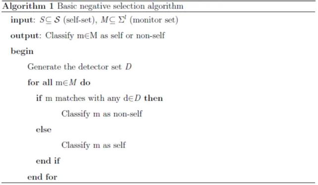
The most generic form of the negative selection can be seen in Algorithm 1 (Figure 3.2). Similar explanation can be found in (Elberfeld & Textor, 2009).
Throughout this section, the following notations will be used: Σl is the universal set of strings, all having a length l. Two partitions of this set, namely S (self) and N
(non-self) are assumed to be known. The inputs that are fed into the algorithm are a sample S⊆ S of self-strings and M⊆Σl, called monitor set which has all strings
that are to be classified. These notations are similar to what is found in Elberfeld and Textor (2011)
S will be used by the algorithm for training and generation of a set of detectors D. An ideal set of D is supposed to have elements that either match with none of the elements inS or it matches with all of the elements in S. The detectors D will then be used for classifying M as self or non-self. An affinity function is used when comparing detector string to a monitor string. Different implementations of such affinity functions exist. Similarly, the generation and representation of the detectors would vary depending on the implementation.
3.3.2.3. r-chunk matching algorithm
A function that would compute the affinity of a detector to any given string is essential in negative selection. Hamming shape-space distance, r-contiguous matching and r-chunk matching are some of the ways of computing this affinity. The r-contiguous and r-chunk matching scheme are the most widely followed
Figure 3.2.: Algorithm 1: Basic negative selection algorithm
approaches associated with negative selection in the literature (Li´skiewicz & Textor, 2010; Stibor, 2009).
r-contiguous matching technique as proposed in Percus, Percus, and Perelson (1993) is a direct adaptation of the technique followed by the T-cells. According this scheme, the detector string matches with any given string, if and only if the detector matches with the given string in at least r continuous positions. The matching characters has to occur at the same indices at the detector and training strings. A generic definition of r-contiguous detectors can be found in Elberfeld and Textor (2009):
Definition 1 (r-contiguous detectors): “An r-contiguous detector is a string d∈ΣL. It matches another string s∈ΣL if there is an i∈{1, . . . , L - r + 1} with
d[i, . . . , i + r - 1] = s[i, . . . , i + r - 1]”
In the case of analyzing network packets, where consecutive characters in a string do not have essentially a semantic correlation between them, r-chunk
matching is a better approach (Balthrop et al., 2002). An r-chunk matching scheme was used when comparing detectors with the test traffic as a part of the
methodology. A generic definition of r-chunk detectors can be found in Elberfeld and Textor (2009):
Definition 2 (r-chunk detectors): “An r-chunk detector (d,i) is a tuple of a string d∈Σr and an integer i∈{1,...,L-r+1}. It matches another string s∈Σl if s[i,...i+r-1] = d”
A number of implementations of r-chunk detector scheme has turned out to have a worst-case space complexity that is exponential of the input self-set size (Elberfeld & Textor, 2009). For example, Stibor, Bayarou, and Eckert (2004), Elberfeld and Textor (2009), and D’haeseleer, Forrest, and Helman (1996) all have exponential running times. This makes the implementation very less practical. As noted earlier, one cannot afford to have high performance and space overheads in IDS systems. The space complexity is mainly because all the implementations tend to generate an exhaustive list of detectors. This becomes more computation
intensive when the self-set is too large. It was argued in Timmis et al. (2008) that this problem is at best an NP-hard one.
It was not until Elberfeld and Textor (2009) that it was proved that this problem could be solved in linear time. Elberfeld and Textor (2009) used patterns to depict a set of strings. That way, the self set and the detector set can be
generated and depicted with lesser time and space overhead. Further optimizations were also proposed in Li´skiewicz and Textor (2010).
Since the r-chunk detectors are represented as strings along with indices, prefix tree is a data structure that is more suited to represent them. This was first introduced in Elberfeld and Textor (2011) and has proven to achieve linear running times for classification. In this research too, the r-chunk detectors are represented as prefix trees and prefix directed acyclic graphs, similar to Elberfeld and Textor
(2011). Both of these concepts are explained in the following section.
1. It has exactly one root node (a node with no inbound edges) and can have one or more leaf nodes (nodes with no outbound edges)
2. All the edges are labeled with characters of the alphabet Σ
3. Each node cannot have more than one edge that is labeled with the same element a∈Σ
4. For a string s, one could say s∈T if there exists a path in T from the root to the leaf node with labels the same as the characters of s.
5. Language L(t) is a set consisting of strings with one or more characters appended to the end of elements of the set T. In other words, each of the strings in L(T) has a prefix string s’∈T (Elberfeld & Textor, 2011). A prefix string s’ of a string s is made of the first n-r characters of s, where r<n, n being the length of the string.
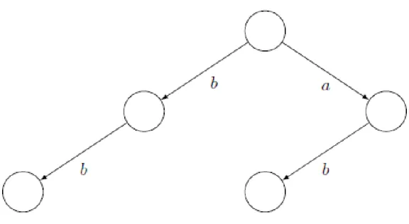
Figure 3.2 is an example of a prefix tree:
Figure 3.3.: An example prefix-tree
For the above example, s=‘bb’∈T because there is a path from the root node to the leaf with these characters as labels. Similarly, s=‘ab’∈T and s=‘aa’∈/T
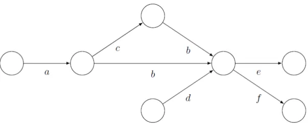
A prefix directed acylic graph (prefix DAG), denoted as D is similar to a prefix tree except that it is a acyclic graph as opposed to a tree. The following are the conditions are to be satisfied for it to be called a prefix DAG:
1. The prefix DAG can have more than one root and leaf nodes 2. All the edges are labeled with characters of the alphabet Σ
3. Each node cannot have more than one edge that is labeled with the same element a∈Σ
4. A string s is said to belong to D, if and only if there is a path from a root to a leaf node labeled the same edges as the string. Note that as opposed to the prefix tree, the prefix DAG can have more than one root and leaf nodes. 5. Language L(d,n) is a set consisting of strings with one more characters
appended to the end of elements of the set D for a given root node n. In other words, each of the strings in L(T) has a prefix string s’∈T (Elberfeld &
Textor, 2011). A prefix string s’ of a string s of length n is made of the first n-r characters of s, where r<n.
Figure 3.3 is an example prefix DAG. For this example, s=‘acbe’, s=‘df’ and s=‘abe’ are some example strings that belong D, because there is a path from a root to a leaf node with those labels on it.
Generation of r-chunk detectors: The following section will discuss the algorithm that would generate the r-chunk detectors. The ultimate aim is for us to achieve O(l) for classification. This is equivalent to the best know performance for negative selection achieved in Elberfeld and Textor (2011). Prefix DAG with failure links will be used representing the detectors. The characteristics and criteria for a prefix DAG is already discussed in the previous section. For a set of monitor strings, each of length l, the algorithm ultimately produces a prefix tree Ti for every index
i∈{1,...,l-r+1} of m. For the self set S, the set of treesTi, will be such that it is a
Figure 3.4.: An example prefix-DAG
Algorithm 2 (Figure 3.5) explains r-chunk detector generation algorithm in detail. First the algorithm begins by creating empty prefix trees, one for each of i∈{1,...,l-r+1}. Once created, the sub-strings (from index position i to the index position i+r-1) of strings in the self set is continuously added onto the
corresponding prefix trees. This is achieved by the lines 8 to 10 in the algorithm. The lines 11 to 13 perform the function of adding new leaf nodes to every non-leaf node with edges labeled with all characters a∈Σ. As per the condition 3 of the prefix trees, no two outbound edges from a node should have the same the labels on them. This is ensured by line 12 of the algorithm. Subsequently, in lines 13 to 15, all the nodes that do not point to the newly generated nodes will be deleted.
The set of all prefix trees generated at the end of algorithm 2 are going to have a Language L(T) that has strings that matches with none of the string in non-self set. For classification of any monitor sting, it could be compared with L(T), which will serve as the detector set. If there is match found for the monitor string with a string in L(T), then it can be classified as self (detector set, L(T) being representative of the self set). Though training takes O(|S |lr|Σ|), the classification can be done in just O(lr) (Elberfeld & Textor, 2011)
But O(lr) has to be further improved for us to match ideal IDS performance. For achieving this, failure links are added to the prefix trees, effectively making
Figure 3.5.: Algorithm 2: Construction of prefix-tree
them graphs (called prefix DAG). This technique was originally proposed in Knuth, Morris, and Pratt (1977) for the purpose of pattern matching in strings. This
technique has evolved and has been applied in a number of researches over the years including Crochemore, Hancart, and Lecroq (2007); Dandass, Burgess, Lawrence, and Bridges (2008); Lin, Lin, Lai, and Lee (2008); Oh, Oh, and Ro (2013); Turing (2006).
The purpose of failure links is to avoid redundant searching of a pattern in a set of trees. When a pattern is not found in a particular tree, it is common to search for the same pattern in the next tree, starting from root node all over again. To avoid this redundant and unnecessary search, failure links are added between the trees, depicting where the search should start in the subsequent tree. This avoids searching from the root node all over again. This model is also proposed as a proof-of-concept in Elberfeld and Textor (2011), which has been implemented here and tested against the real-world network traffic. The algorithm followed in this research is explained in Algorithm 3 (Figure 3.6).
Figure 3.6.: Algorithm 3: Construction of prefix-DAG
As shown in Algorithm 3 (Elberfeld & Textor, 2009), the failure links are generated for the set of prefix trees. For every tree, choose a pair of ‘n’ and ‘a’, where ‘n’ is the node in the tree and ‘a’ is the character that is not labeled on any of the outgoing nodes of ‘n’ (Elberfeld & Textor, 2009). If s is the string that is formed
by the labels of edges from the root of the tree to the node ‘n’, for a string s’ = sa. Say, there is a path from n to n’ that would point to such a string, n’ being the node in the next tree, form an edge connecting n and n’. This is an example of a failure link. Form failure links for each of the nodes in subsequent trees, when the above conditions are satisfied. These failure links will help in expediting the search process (Elberfeld & Textor, 2009).
3.3.2.4. n and r values
n and r values are the most important parameters in r-chunk matching algorithm. n value is the length of the string in training dataset that will be used for generation the detectors. For a given training dataset, larger n value does not essentially mean a better detection rate. Because in some datasets, larger n value would mean larger noise is included in training. An example of noise in the context a network packet can be values of optional headers which do not essentially help in the detection of attacks. Also, larger n value would mean higher processing and storage overhead associated with training process, because larger strings are processed. Similarly, if n value is set too small, it would lead to generation of detectors which are not essentially representative of the training dataset.
r value controls the length of the detectors that will be generated. In our algorithm, since detectors are represented as DAGs, larger r value would mean larger DAGs. In theory, ideal r value is one that is closest to n (Esponda, Forrest, & Helman, 2004). But since the generation of detectors is an exponential algorithm, higher r value would have a disastrous effect on the performance (Esponda et al., 2004; Stibor et al., 2005). For this reason, r value was varied from 40% of n up to 80% of n and the corresponding results analyzed.
3.3.3 Testing the Intrusion Detection System
3.3.3.1. Detection and false alarm rates
Parameters like true and false positives rates, true and false negatives rates are the most important parameters of any IDS. As pointed out in the previous sections, these parameters are a measure of the effectiveness of the detection mechanism of an IDS. For the given dataset, the results of these parameters were analyzed for different thresholds and r-values.
It is to be noted that higher false negative rate can be tolerated as compared to higher false positive rate (Hofmeyr, Forrest, & Somayaji, 1998). This is because, false negatives can be solved by adding additional detection mechanisms and additional layers of security. But false positives cannot be solved in a similar manner. On the other hand, layering will only compound the false positives
problem. In statistical theory, false negatives are type I errors and false positives are type II errors (Storey, 2003).
The formulae used for the calculation of these rates is the same as used in Portnoy, Eskin, and Stolfo (2001). Detection rate is calculated from the number of true positives divided by the total number of non-self instances in the test dataset (Portnoy et al., 2001). False positive rate is calculated from the number of false positives divided by the number of normal (self) instances in the test dataset
(Portnoy et al., 2001). False negative rate is defined as the number of false negative instances divided by the total number of anomalous (non-self) instances in the test dataset (Portnoy et al., 2001).
3.3.3.2. ROC curve analysis
Introduced in Axelsson (1999), Receiver Operating Characteristics (ROC) curves are important benchmarks of the effectiveness of IDS systems. An ROC curve is a plot of the false positive rate against the detection rate. A convex ROC
curve is a sign of effective detection mechanism. Concave curve implies so-called ‘holes’ in the IDS that might lead to high false negative rates. Rapid drops in the curve is also a sign of weakness in the IDS.
It is to be noted that at worst operating conditions, the IDS can claim none of its inputs to be an attack. In such case, the detection rate and also the false positive rate will be 0. On other hand, if the IDS claims each and every input to be an attack, the detection rate and false positive rate will be 1 (100%). Hence
theoretically, the points (0,0) and (1,1) will be a part of any ROC plot (Axelsson, 1999; Chen, Hsu, & Shen, 2005).
3.3.4 Testing Environment
The developed Java application was packaged as a JAR file and run on a Virtual Machine running on a ESXi server. The VM used was Kali Linux environment with a Java version of 1.8.0. Since the program would have high memory requirements, the VM was installed with a RAM capacity of 40GB and hard disk capacity of 120GB. The number of logical processors allocated were 12. The VM was isolated from the outside network with appropriate packet filtering rules on a Packet Fence firewall. Since the implementation was done in Java, the application can be tested on other platforms as well.
3.4 Summary
This chapter provided the framework and methodology used in the research study.
CHAPTER 4. RESULTS AND ANALYSIS
The NSL-KDD dataset is an improvement over the original KDD cup dataset (Revathi & Malathi, 2013). More details about this dataset were discussed in the previous chapter. The developed IDS was tested against the NSL-KDD dataset and parameter values like false positives, false negatives and detection rates were
calculated. ROC curves were also plotted for the obtained results. Testing was repeated with different values of n, r, and anomaly threshold values and the corresponding rates were calculated.
4.1 Processing data
Some pre-processing had to be done on the dataset before testing it on the IDS. Since the negative selection module accepts only self traffic as an input for training, a Python script was written to retrieve only the normal traffic from the labeled training data. Also, since the self data has to have strings that are of the same length, the records were padded with the character ‘0’ so that all the records were the length of the largest string in the file. Similarly, a different Python script was used for calculating false positive, false negative, and detection rates from the logs of the developed IDS. This was because, the developed IDS reads the test traffic and only classifies each record as ‘normal’ or ‘anomaly’, based on several factors discussed earlier. This result has to be compared with the labeled test data to calculate the detection rates.
4.2 Detection and false alarm rates
False positive and detection rates were calculated by running the test data in the NSL-KDD dataset. These rates were obtained for different n, r and threshold values. Since the length of strings in the test dataset was 152 (including the added padding), the n values tested were between 70 and 120. Higher n values only
resulted in poorer detection rates and insufficient heap memory. As stated earlier, r values were tested between 40% and 80% of the given n value. Anomaly threshold was varied between 10% and 100%. Highest detection rate obtained was 81.56% for n=100, r=40 and threshold = 20%. But the corresponding false positive rate was also high at 39.52%.
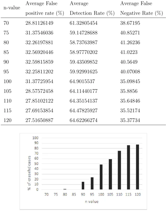
By varying the above mentioned parameters, the false alarm and detection rates were calculated. Table 4.1 shows the different average rates for given n values. It can be seen than an n value of 100 yields the best average detection rate of 64.90%. But this also resulted in a moderate average false positive rate of 31.37%. As n value was increased above 100, the average detection rate started to decline. This may be attributed to the increased noise being included for generation of detectors. Also with higher n values, the system ran out of heap space and crashed abruptly. This can be attributed to huge storage overhead associated with
generation of large detectors. The percentage of test cases crashed for given n values can be seen in the Figure 4.1.
4.3 ROC Curves
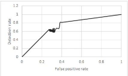
As mentioned in the previous chapter, ROC curves are plots of detection rates against false positive rates. Such curves indicate the operating region of an IDS and also lets the network administrator decide on the operating region that is suitable for a given network environment. As mentioned earlier, the points (0,0) and (1,1) occur at the worst operating conditions of any IDS. Figure 4.2 shows the ROC
Table 4.1: Comparison of average rates for given n values
n-value Average False positive rate (%) Average Detection Rate (%) Average False Negative Rate (%) 70 28.81126149 61.32805454 38.67195 75 31.37546036 59.14728688 40.85271 80 32.26197881 58.73763987 41.26236 85 32.56920446 58.97770202 41.0223 90 32.59815859 59.43509852 40.5649 95 32.25811202 59.92991625 40.07008 100 31.37725954 64.9015537 35.09845 105 28.57572458 64.11440177 35.8856 110 27.85102122 64.35154137 35.64846 115 27.69153854 64.47825927 35.52174 120 27.51650887 64.62266274 35.37734
Figure 4.1.: Percentage of crashed test cases Vs. n value
curve for the tested dataset with these two points. This curve was plotted using about 565 tested cases, obtained by varying n, r and threshold values.
Figure 4.2.: ROC curve including points (0,0) and (1,1)
Figure 4.3 shows the actual ROC curve without the points (0,0) and (1,1). This curve is generally convex and does not have abrupt drops in slope. The region from false positive rate of 0.27 to slightly after 0.32 can be considered as ideal operating region for this IDS. With the increase in false positives beyond 0.27, there is no abrupt drop in detection rate, indicating a wide operating region with decent false positive and detection rate. There is a slight concave region in the curve where false positive rate is 0.37. This is a sign of poor detection mechanism in that region, but since it is outside the ideal operating region of the IDS where the false positive rate is already higher, this is not a huge compromise on the effectiveness.
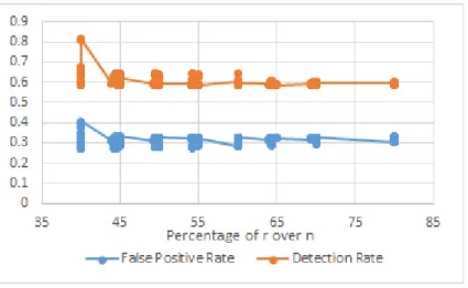
4.4 Effect of r-value on detection and false positive rates
The r values tested ranged from 40% to 80% of the value of n (calculated from (r/n)*100). The false positive and detection rates against various r value percentages can be seen in the Figure 4.4. Individual detection rate (at 81.56%) and average detection rate (at 62.68%) were the maximum when the r value was 40% of n value. But the average false positive rate was also slightly higher at 30.50%. It is to be noted that these are values are specific to the NSL-KDD dataset and may not
Figure 4.3.: ROC curve
always be true for another dataset. Ideal r and n values for a different dataset can be deduced by similar testing.
Figure 4.4.: False positive and detection rates against percentage of r values over n
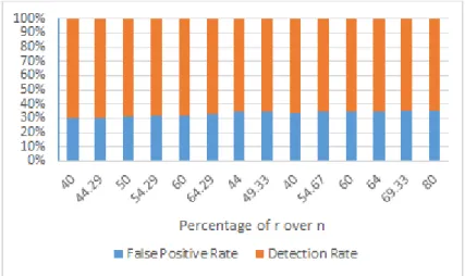
Figure 4.5 shows the comparison of false positives and detection for different r values and constant n and threshold values. This graph shows the direct effect of r value on the detection rate. The n value was set at 75 and threshold value was set at 70%. It could be observed that as the r value increases, detection rate decreases
and the false positive rate increases. As already seen in Figure 4.1, higher n values resulted in heap space running out and the program crashing. The insufficient heap space issue further increased with higher r values. It can be concluded that for the NSL-KDD dataset, the effectiveness and performance of the IDS decreases beyond an r percentage of 40%.
Figure 4.5.: False positive and detection rates against percentage of r values over n (constant n and threshold values)
4.5 Comparison of effectiveness with other IDS systems
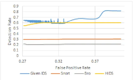
The Figure 4.6 shows the ROC curves of the developed IDS along with the other prominent IDS systems like Snort (Alder et al., 2007), Bro (Paxson, 1999), Hybrid Intrusion Detection System (HIDS) proposed in Hwang, Cai, Chen, and Qin (2007). ROC curves for these three IDS systems were already compared in Hwang et al. (2007). HIDS is a combination of anomaly-based and signature-based
detection mechanisms and would serve as a proper comparison. As seen in the figure, Snort and Bro have an operating region with relatively lower detection rates. This is because the NSL-KDD dataset has over 90% of the attacks in the test
dataset that is not directly present in the training dataset. This is huge shortcoming for Snort and Bro IDS systems that are largely signature-based detection systems.
HIDS having a combination of anomaly based and signature based detection mechanisms, performs better overall compared the other three IDS systems. The operating range of HIDS has a detection rate around 30% better than Snort and around 38% better than Bro. In comparison with the developed IDS, HIDS has almost an identical detection rate range in the operating region before a false positive rate of 0.32. It is to be noted that the developed IDS has only anomaly based defenses and uses only self traffic for training, while the other IDS systems use both self and non-self traffic while training. It could be argued that considering the above aspects, the developed IDS is relatively more effective than HIDS for NSL-KDD dataset.
Figure 4.6.: ROC curves - comparison against other IDS systems
4.6 Effectiveness against zero-day attacks
We know that the greatest strength of anomaly-based IDS systems is their capability to detect newer forms of attacks like zero-day attacks. This makes it critical for us to study the effectiveness of the developed IDS against such attacks.