Seasonal Stochastic Volatility: Implications for the pricing of commodity options

(1)

Seasonal Stochastic Volatility:

Implications for the Pricing of

Commodity Options

Juan C. Arismendi,

∗

Janis Back,

†

Marcel Prokopczuk,

‡

Raphael Paschke,

§

and Markus Rudolf

¶,‖

Abstract

Many commodity markets contain a strong seasonal component not only at the price level, but also in volatility. In this paper, the importance of seasonal behavior in the volatility for the pricing of commodity options is analyzed. We propose a seasonally varying long-run mean variance process that is capable of capturing empirically observed patterns. Semi-closed-form option valuation Semi-closed-formulas are derived. We then empirically study the impact of the proposed seasonal stochastic volatility model on the pricing accuracy of natural gas futures options traded at the New York Mercantile Exchange (NYMEX) and corn futures options traded at the Chicago Board of Trade (CBOT). Our results demonstrate that allowing stochastic volatility to fluctuate seasonally significantly reduces pricing errors for these contracts. JEL classification: G13

Keywords: Commodities, Seasonality, Stochastic volatility, Options pricing, Natural gas, Corn

∗_{Faculty of Economics, Federal University of Bahia, R. Bar˜ao de Jeremoabo, 6681154}

-Ondina, Salvador - BA, 40170-115, Brasil

†_{Department of Finance, WHU – Otto Beisheim School of Management, 56179 Vallendar,}

Germany. e-mail: [email protected]

‡_{School of Economics and Management, Leibniz University Hannover, Koenigsworther Platz}

1, 30167 Hannover, Germany

§_{University of Mannheim, L5-2, 68131 Mannheim, Germany.} _e-mail:

[email protected]

¶_{Department of Finance, WHU – Otto Beisheim School of Management, 56179 Vallendar,}

Germany. e-mail: [email protected]

‖_{Part of this work was completed while Janis Back was visiting Princeton University. He}

(2)

I

Introduction

Trading in commodity derivatives markets has experienced a tremendous growth over the last decade.1 _{Increased volatility of commodity prices created the need}

for efficient risk management strategies. The ability to efficiently manage these price risks has direct consequences for the profitability of many companies and economic growth. Commodity options provide a powerful risk management tool, but accurately pricing these contracts is not a trivial task as the main input factor, the volatility, is not observable. Therefore, the accurate modeling of volatility in these markets is of critical importance.

Many commodities exhibit significant seasonal variations in at least two ways. First, there can be seasonality at the price level (of futures and/or the spot price). This pattern can be observed as cyclical behavior in the time series of prices or also in the cross-section of futures prices, i.e. in the futures curve. Second, the second moment, i.e. the variance, may also vary seasonally. This pattern can be observed in the volatility surface of commodity options. However, most of the existing literature concerning the pricing of commodity contingent claims solely considers the crude oil market or other markets without seasonality, such as copper or gold. Brennan and Schwartz (1985), Gibson and Schwartz (1990), Schwartz (1997), Schwartz and Smith (2000), and Casassus and Collin-Dufresne (2005) develop one-, two-, and three-factor models in a Gaussian framework and

1

See, e.g., Tang and Xiong (2012).

(3)

study the empirical performance for pricing crude oil, copper, gold, and silver futures.

Sørensen (2002) adds a seasonal component at the price level to the constant volatility two-factor model of Schwartz and Smith (2000) and applies it to the wheat, corn, and soybean markets. Similarly, Manoliu and Tompaidis (2002) and Cartea and Williams (2008) apply this model to the US and UK natural gas futures market, respectively.

However, Anderson (1985) and Choi and Longstaff (1985) already note that commodity markets exhibit a second type of seasonality, i.e. the seasonal variation of volatility.2 Back et al. (2013) consider this fact in the context of pricing commodity options. They show that considering seasonality in the volatility greatly improves the pricing performance for several agricultural and energy options. However, Back et al. (2013) assume that volatility is deterministic, which is clearly a very strong assumption as it cannot generate the volatility smile, which is also observed in commodity markets.3

Trolle and Schwartz (2009) develop a Heath, Jarrow, and Morton (1992)-type stochastic volatility model for the pricing of commodity futures and options but do not consider seasonality as they apply their model only to the crude oil market. The only articles allowing for seasonal and stochastic volatility we are aware of are Geman and Nguyen (2005) and Richter and Sørensen (2002), who

2

See also Khoury and Yourougou (1993), Routledge et al. (2000), Suenaga et al. (2008), Karali and Thurman (2010) and Ovararin and Meade (2010) for analyses of seasonal volatility in commodity markets. See Doshi et al. (2011) for modeling seasonal volatility in general.

3

(4)

consider the pricing of soybean futures and options. However, calculating prices of futures and options in their model framework is computationally very burdensome. Accordingly, they do not empirically study the options pricing ability of their models at all.

In this paper, we propose an extension of the Heston (1993) stochastic volatility model that reflects the seasonal nature of volatility. We incorporate the seasonality within the long-term mean to which the variance process reverts. In contrast, the models proposed by Geman and Nguyen (2005) and Richter and Sørensen (2002) model the seasonality as a cyclical behavior of the underlying short-term shocks. Since the movements of the underlying source of risk are stable over the years and furthermore driven by factors outside the financial system, we consider our approach to model seasonality as a recurrent long-term phenomenon economically more plausible. Besides, our model has the crucial advantage of enabling us to compute option values in an efficient way, which is of significant importance if one wants to apply the model in practice. This fact allows us to empirically study the pricing performance of our model using an extensive data set of options prices.

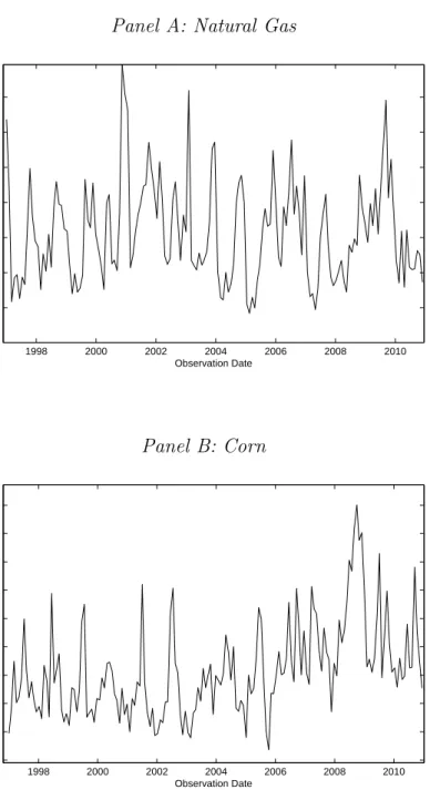
Our model is applicable to every commodity market exhibiting seasonality in volatility. In our empirical analysis, we focus on the natural gas and corn markets, both being prominent examples of markets with stochastic and seasonal volatility. Historical volatilities of natural gas and corn front-month futures are shown in Figure 1. It can be seen that volatility is far from being constant over

(5)

time. In fact, volatility seems to fluctuate stochastically while following a very pronounced seasonal pattern.4 _{For energy markets like the natural gas market,}

weather-induced demand shocks lead to a higher volatility of futures prices during the fall/winter. For agricultural commodities like corn, volatility is primarily driven by the supply side and is usually highest during the spring/summer prior and throughout the harvesting period when inventory levels are low and significant uncertainty regarding the new harvest is resolved.

We use a large data set of New York Mercantile Exchange (NYMEX) natural gas options and Chicago Board of Trade (CBOT) corn options as well as the corresponding futures contracts for both markets. The time period covered by the options data is from January 2007 to December 2010 and consists of 367,469 option price observations for natural gas and 93,325 observations for corn. Additionally, we employ ten years of futures data for both markets spanning the period from January 1997 to December 2006 to estimate our model under the physical measure using a Bayesian Markov Chain Monte Carlo (MCMC) approach. In doing so, we follow Bates (2000) and Broadie et al. (2007) and abstain from a pure cross-sectional (re)-calibration exercise as in Bakshi et al. (1997) but estimate all parameters that should be equal under the physical and the risk-neutral measure from a long time series of historical data.

The results of our empirical study show that our model is superior for the pricing of commodity options with seasonalities. Compared to the standard

4

(6)

stochastic volatility model of Heston (1993), our model yields substantial improvements in pricing accuracy. The same holds true for the comparison with the seasonal deterministic volatility model of Back et al. (2013). The results obtained are both statistically and economically significant and consistent for different robustness checks, implying that the proposed seasonal model should be considered when valuing options on commodities that undergo a seasonal cycle.

The remainder of this paper is organized as follows. Section II lays out the model for pricing options under seasonal volatility. Section III describes the data set and the estimation approach. Section IV presents and discusses the empirical results. Section V concludes. The Appendix contains additional details on the numerical implementation of the model.

II

Model Description

In this section, we present a stochastic volatility model that incorporates a seasonal adjustment of the variance process to capture the empirically observed seasonal behavior of many commodities. After introducing the price and variance dynamics, we derive the valuation formula for European call options.

A. Commodity Futures Price Dynamics

The underlying of almost any exchange traded commodity option is not the commodity’s spot price but the price of a corresponding futures contract. We

(7)

therefore start by specifying the dynamics of the futures price. The alternative approach would be to make an assumption on the dynamics of the spot price and derive the futures price dynamics within this model. However, this approach has the severe disadvantage that it is generally not possible to derive a closed-form solution for the commodity futures price in a stochastic volatility framework, which hinders the derivation of a computationally efficient options pricing formula.5 _The

commodity futures price dynamics under the physical measure are assumed to follow dFt(T) = µFt(T)dt+Ft(T) p VtdWF,t (1) dVt = κ(θ(t)−Vt)dt+σ p VtdWV,t (2) θ(t) = θ eηsin(2π(t+ζ)) (3)

where Ft(T) is the futures price at t with maturity T and µis the drift of the

futures price process under the physical measure. Vt is the instantaneous variance

of the futures returns described through a square-root process as used by Cox et al. (1985),κis the mean-reversion speed of the variance process,θ(t) is the long-term variance level to which the process reverts, and σis the volatility-of-volatility parameter. WF,t and WV,t are two standard Brownian motions with instantaneous

5

The reason that it is not possible to derive a closed-form futures pricing formula is that the spot commodity is usually assumed to be non-tradable and therefore the market is incomplete (see, e.g., Schwartz (1997)). Furthermore, empirical studies have demonstrated that a second, mean-reverting factor is needed to properly price futures contracts. The mean-reversion property together with volatility being stochastic prohibits the derivation of a closed-form futures pricing formula (see Richter and Sørensen (2002) and Geman and Nguyen (2005)). In contrast, as the futures contract is clearly tradable, no mean-reversion can prevail under the risk-neutral measure as otherwise arbitrage opportunities would exist.

(8)

correlationρ.6 _{A sufficient condition to enforce the positivity of the variance process}

is 2κθe−η ≤σ2_.

If we set θ(t) to be constant, the model is identical to the stochastic volatility model of Heston (1993). However, in contrast to Heston’s model, the long-term variance parameterθ(t) is generalized to be a function of time. The long-term mean variance level is assumed to beθ, which is superimposed by a seasonal component as defined in Equation (3). The shape of the seasonal adjustment is specified by two parameters: the size of the seasonal effect is governed by η (amplitude of the sine-function) and ζ (shift of the sine-function along the time-dimension). To ensure the parameters’ uniqueness, we impose η _≥0 and ζ _∈[0,1], while January 1 represents the time origin.

In general, the model setup allows θ(t) to be of any functional form. We use the simple trigonometric function as it provides a reasonable compromise of good fit to the annual volatility pattern observed for many seasonal commodity markets while introducing only two additional parameters, facilitating model estimation in empirical applications.7 _{In the following, we will refer to this Seasonal Stochastic}

Volatility Model as the SSV Model_{. For a zero amplitude, i.e.} _η _{= 0, the} SSV Model_{nests a non-seasonal specification of this Stochastic Volatility Model,}

labeled as SV Model_.

6

One might also consider models with non-Gaussian innovations as analyzed, e.g., by Nakajima and Omori (2012) and Abanto-Valle et al. (2015). However, this would complicate the valuation of options severely as no closed form formula is known in these cases.

7

In Subsection IV.D.we consider more complex trigonometric functions. This leads to some improvements for natural gas, but not for corn.

(9)

B. Valuation of Options

To derive the pricing formula for European call options, we change to the risk-neutral measure. Assuming market prices of risk, λp(Vt), for the variance process,

we obtain dFt(T) = Ft(T) p VtdW Q F,t (4) dVt = [κ(θ(t)−Vt)−λVt]dt+σ p VtdW Q V,t (5) θ(t) = θ eηsin(2π(t+ζ)). (6)

W_F,tQ and W_V,tQ are standard Brownian motions under the risk-neutral measure with instantaneous correlation ρ. Under the risk-neutral measure, the futures price has to be a martingale and hence, the price process exhibits a drift of zero. Furthermore, since the seasonality due to weather conditions by itself is no systematic risk factor, there is no price of risk associated with it which would change the parameters of the long-term seasonality process.8 _{Notwithstanding,}

whether weather conditions turn out favorably or not, is priced by λ.

We have extended Heston’s model by allowing the long-term variance level to vary over the calendar year in a deterministic fashion. Therefore, the fundamental partial differential equation is, except for the time dependence, identical to Heston’s solution. Any claim U on F must satisfy

∂U ∂t + 1 2F 2_V ∂2U ∂F2 + [κ(θ(t)−V)−λV] ∂U ∂V + 1 2V σ 2∂2U ∂V2 +σρF V ∂2U ∂V ∂F = 0. (7) 8

(10)

Assuming constant interest rates, Heston derives a quasi-closed-form solution for European call options in terms of characteristic functions, which for futures contracts is given as C(F, K, V, T) =e−r(T−t) [F P1−KP2] (8) with Pj = 1 2+ 1 π Z ∞ 0 Re eiφlnKfj(F, V, t, T, φ) iφ dφ, j = 1,2 (9)

where C is the price of a European call option on a futures contract F at time t with strike price K and maturity T; i denotes the imaginary unit, Re [.] returns the real part of a complex expression, and fj is a characteristic function.

As shown by Heston (1993) and more generally by Duffie et al. (2000), the characteristic function solution is of the form

fj =eAj(T

−t,φ)+B_j(T−t,φ)V+iφlnF

. (10)

(11)

Aj(τ, φ) andBj(τ, φ) to be solved reads ∂Bj ∂τ = 1 2σ 2_B2 j −(bj −ρσφi)Bj +ujφi− 1 2φ 2 ₍₁₁₎ ∂Aj ∂τ =κθ(τ)Bj (12) where u1 = 1₂, u2 =−1₂,b1 =κ+λ−ρσ, and b2 =κ+λ.

The important aspect to note is that only the second ODE is affected by our model extension as the long-term variance level does not appear in the first ODE. Consequently, the solution of Equation (11) remains unchanged from Heston’s solution and can be found in the Appendix.

The solution of Equation (12) can be expressed by means of the hypergeometric function. However, we found that a direct numerical integration is the fastest way to solve this ODE while maintaining high precision.9 _{In general, it should be noted}

that the proposed model extension is well tractable with regard to its computational demand, rendering real-world applications feasible. Details on the implementation are given in the Appendix. Prices for European put options can easily be obtained through put-call-parity.

9

In the case of theSV Model_{, the closed-form solution for this ODE is of the form}Aj(τ, φ) = κθ σ2 h (bj−ρσφi+d)τ−2 ln ₁ −gedτ 1₋g i .

(12)

III

Data Description and Estimation Procedure

A. Data

For our empirical study, we use a data set consisting of daily prices of physically settled natural gas and corn futures and American-style options written on these futures contracts traded at the NYMEX and the CBOT, respectively. In the case of natural gas, a short position in the futures contract commits the holder to deliver 10,000 million British thermal units (mmBtu) of natural gas at Sabine Pipe Line Co.’s Henry Hub in Louisiana. Prices are quoted as US dollars and cents per mmBtu. In the case of corn, the contract unit of a futures is 5,000 bushels and the prices are quoted as US cents per bushel.10 _{As interest rates, we use the}

3-month USD Libor rates published by the British Bankers’ Association. All data are obtained from Bloomberg.

The futures data sets span the time period from January 2, 1997 to December 31, 2010, whereas our options data sets span the period January 3, 2007 to December 31, 2010 and comprises 1,008 trading days. Call and put options and the corresponding futures contracts are available with maturities in each calendar month for natural gas while corn futures and options are only available for maturities in March, May, July, September, and December. Therefore, we use options with delivery months from February 2007 to December 2011 for natural

10

See the webpage of the CME group, www.cmegroup.com, for details on the contract specifications.

(13)

gas and from March 2007 to December 2011 for corn. While trading in the futures contract ceases three business days prior to the first day of the delivery month for natural gas, the last trading day of the corn futures is the business day prior to the 15th calendar day of the contract month.11

The minimum price fluctuation for the natural gas options is $_{0.001 and for}

corn it is$_{0.00125. Due to this discreteness in reported prices, we exclude options}

with a price of less than $_{0.01. Furthermore, following Doran and Ronn (2008)}

and Trolle and Schwartz (2009), we exclude options being very close to expiration and long-term contracts since for these open interest is usually lower and liquidity tends to be low as well, i.e. we consider options with a maturity of at least 15 and not more than 365 days. For the same reasons, we only consider options with a moneyness between 90 % and 110 %.

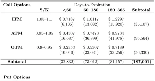
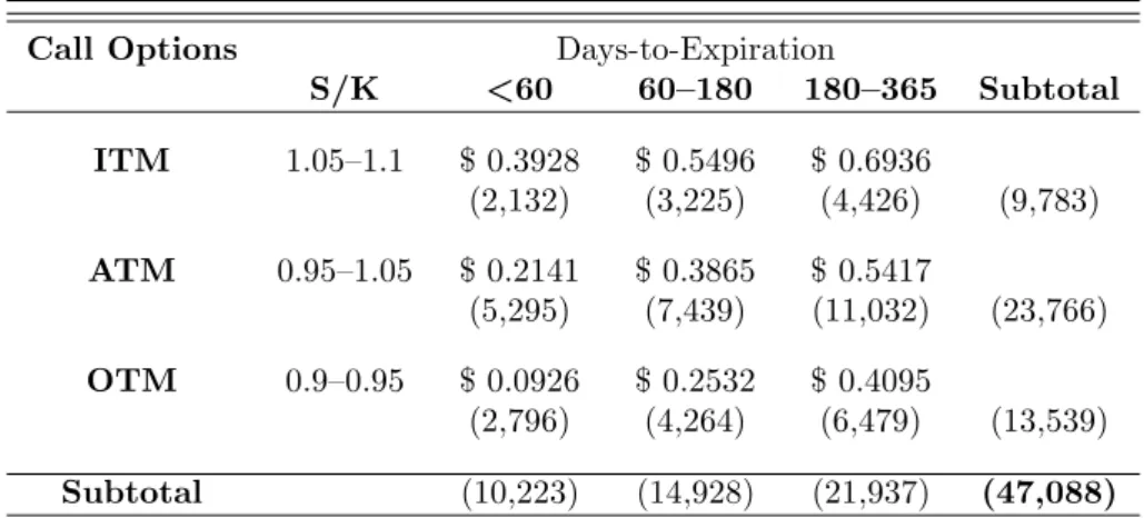
Tables 1 and 2 summarize the properties of the call and put options comprising our data sets. The total number of observations is 367,469 for natural gas and 93,325 for corn. We divide these data sets in different moneyness and maturity brackets for the subsequent analysis. We refer to a call (put) option as out-of-the-money, OTM, (in-out-of-the-money, ITM) when the price of the futures contract is between 90 % and 95 % of the option’s strike price. When the price of the futures contract is between 95 % and 105 % of the option’s strike price, options are considered to be at-the-money, ATM. Finally, for futures prices between 105 % and

11

Trading in the natural gas options ends on the business day before the last trading day of the futures while for corn the last options trading day is the last Friday which precedes by at least two business days the last business day of the month preceding the expiry month (Source: www.cmegroup.com).

(14)

110 % of the option’s strike price, call (put) options are referred to as ITM (OTM). We consider options with less than 60 days to expiration as short-term, options with 60 to 180 days to expiration as medium-term, and options with 180 to 365 days to expiration as long-term.

The pricing formulas obtained in Section II are for European options while the options in our data set are of the American-style. To take this aspect into account, we follow Trolle and Schwartz (2009) and transform each American option price into its European counterpart by approximating the early exercise premium using the procedure developed by Barone-Adesi and Whaley (1987). Since the adjustment is carried out for each option separately, the options’ price characteristics should not be altered and our analysis should not be affected, even though the analytical approximation approach of Barone-Adesi and Whaley (1987) is based on a constant volatility framework in contrast to the present stochastic volatility setting.12 _{As we}

only consider options with a time to maturity of not more than one year and the considered strike range excludes options which are deep ITM, the American-style feature is of limited importance. Based on the approximation of Barone-Adesi and Whaley (1987), the average premium for the right of early exercise amounts to only 0.28 % of the options value for natural gas and 0.26 % for corn.

12

Refer to Trolle and Schwartz (2009) for a more detailed discussion and justification of this approach.

(15)

B. Estimation Approach

Every stochastic volatility model poses a substantial estimation problem as the volatility path is not observable. Therefore, one needs to estimate not only the model parameters but also the latent volatility process. A standard approach found in numerous articles is based on a pure cross-sectional calibration, such as in Bakshi et al. (1997). For each observation date, one minimizes an objective function to fit the observed option prices on that particular date. This procedure is repeated for every observation date and, thus, allows the parameters to fluctuate freely through time, which is, of course, inconsistent with the assumed model dynamics in which the parameters are assumed to be constant.

To reduce this inconsistency and to make better use of available information, we follow a different approach which has been suggested by Bates (2000) and Broadie et al. (2007) and comprises a two-step procedure. The first step consists of estimating all parameters that should be equal under the physical and the risk-neutral probability measure using return observations. We therefore make use of a long time series of data to infer most of the model parameters. Given these parameters, we use in a second step the cross-section of options data to estimate the risk premium λ and the current variance level Vt.13

Since the volatility process is not observable, simple estimation methods such

13

A third possibility is to estimate all parameters jointly from a time series of returns and options prices, as in Eraker (2004). However, as Broadie et al. (2007) point out, this approach is hindered by the computational burden and substantially constrains the amount of data that can be used. For example, Eraker (2004) restricts his analysis to an average of three options per day.

(16)

as maximum likelihood methods cannot be applied for the first step. Therefore, we follow Jacquier et al. (1994) and Eraker et al. (2003) and apply an Markov Chain Monte Carlo (MCMC) estimation approach, which is a Bayesian simulation-based technique. This approach allows us to estimate the unknown model parameters and the unobservable state variables, i.e. the volatility path, simultaneously.14

In order to be able to estimate the models, it is necessary to express them in discretized form. Defining Yt = lnFt and using a simple Euler discretization, we

get under the physical measure15

Yt =Yt−∆t+µ(t)∆t+

p

Vt−∆tε

Y

t (13)

and for the variance process

Vt =Vt−∆t+κ(θ(t)−Vt−∆t)∆t+σ p Vt−∆tε V t. (14) The innovations εY

t and εVt are normal random variables, i.e. εYt ∼ N(0,∆t) and

εVt ∼ N(0,∆t) with correlation ρ. The series Yt is constructed by concatenating

futures prices with different maturity months, yielding a series of futures prices with almost constant maturity. As this price series also contains a seasonal component, we allow the mean drift to fluctuate seasonally by settingµ(t) =µ+φsin(2π(t+ξ)). For the SV Model_{, we set} _{θ(t) =} _θ _{and for the} SSV Model _{we set} _{θ(t) =}

14

For an excellent overview of MCMC estimation techniques with financial applications, see Johannes and Polson (2006).

15

(17)

θ eηsin(2π(t+ζ))_{. In the following implementation, we estimate both models using}

daily data.

The main piece of interest in Bayesian inference is the posterior distribution p(Θ, V_|Y) which can be factorized as

p(Θ, V_|Y)_∝p(Y_|V,Θ)p(V_|Θ)p(Θ) (15)

where Y is the vector of observed log prices, V contains the time series of volatility, Θ is the set of model parameters, p(Y_|V,Θ) is the likelihood, p(V_|Θ) provides the distribution of the latent volatility, and p(Θ) is the prior, reflecting the researcher’s beliefs regarding the unknown parameters. The MCMC method provides a way to sample from this high-dimensional complex distribution. The main idea is to break down the high-dimensional posterior distribution into its low-dimensional complete conditionals of parameters and latent factors which can be efficiently sampled from. The output of the simulation procedure is a set ofGdraws,

{Θ(g)_{, V}(g)_}

g=1:G, that forms a Markov chain and converges to p(Θ, V|Y). Given

the sample from p(Θ, V_|Y), information about individual parameters can then be obtained from the respective marginals of the posterior distribution. Whenever possible, we use conjugate priors and apply a Gibbs sampler.16 _{The basic} _SV

Model _{is identical to the model analyzed in Eraker et al. (2003); we therefore}

follow their prior specifications. The distribution of Vt is non-standard but can be

16

(18)

sampled using a random walk Metropolis algorithm which is calibrated to yield an acceptance probability between 30 % and 50 %.17 _{For the seasonal parameters, we}

use a Gibbs sampler with an exponential prior for the magnitude of seasonality, η, and an independence Metropolis algorithm with a uniform density over the unit interval as the proposal density for the shift of the seasonality, ζ. We use 1,000,000 simulations, i.e. G =1,000,000, and discard the first 400,000 as “burn-in” period of the algorithm.

Given the structural model parameters estimated under the physical measure, the market price of risk λ and the current variance level Vt can be inferred from

options data in the second step of our estimation procedure. Thereby, theoretical option prices can be obtained using the pricing formulas presented in Section II.

The two quantities λ and Vt are estimated by minimizing a loss function

capturing the fit between the theoretical model prices and the prices observed at the market. We follow Broadie et al. (2007) and use the root mean squared errors (RMSE) of implied volatilities (IV-RMSE) as the objective function, i.e.

Φ∗

t = arg min

Φt

IV-RMSE(Φt) = arg min

Φt v u u t 1 Nt Nt X i=1 ( ˆIVt,i(Φt)−IVt,i)2. (16)

Here, IVt,i is the implied Black (1976) volatility of the observed market price and

ˆ

IVt,i(Φt) is the implied volatility of the theoretical model price. Nt denotes the

number of contracts available at date t and Φt = {λ, Vt} the unknown quantities

17

(19)

to be estimated.18

Minimizing the implied volatility metric provides an intuitive way of weighting all observations more or less equally. Another metric that also is very popular in the literature, as used e.g. by Bakshi et al. (1997), is the root mean squared error of prices ($_{-RMSE) which uses the observed quantities directly and is therefore}

‘model-free’. However, it puts more weight on the more expensive ITM options and on options having a longer time to maturity. The opposite is true for the relative root mean squared error of prices (RRMSE). In general, the applied loss function should be chosen corresponding to the objective of the decision maker. E.g. for an investor with a long-term ITM options portfolio, the $_{-RMSE error metric might}

be most appropriate while in other applications a different loss function might be preferred. For robustness reasons, we have applied all three loss functions in our analysis. However, we focus mainly on the IV-RMSE when presenting the results in Section IV since this measure applies a similar weighting for all observations. The other results are summarized in Subsection IV.E.

18

For the numerical estimation of the two parameters,Vtwas limited to the interval 0 to 2 and

λwas restricted not to exceed an upper boundary of 100 while the lower boundary is given by

−κto ensure the mean-reversion property of the variance process. One should note, however, that these artificial boundaries were non-binding in almost all cases. In particular, for theSSV Model_{, only the artificial upper boundary for}Vtwas binding during two periods of significant

market volatility in the case of natural gas (less than 1.5 % of the 1,008 trading days in our sample) and never binding in the case of corn. The boundaries forλwere never binding in either market.

(20)

IV

Results

In this section, we report the results of our empirical study. After discussing the parameter estimates obtained for the two models, we present in-sample and out-of-sample results regarding the models’ options pricing performance. Next, we briefly compare the results for the stochastic volatility models to the seasonal deterministic volatility model of Back et al. (2013). Then, we consider more complex seasonality functions. At the end of this section, we provide information on further robustness checks conducted.

A. Estimated Parameters

In the first step of the estimation procedure, the structural model parameters are estimated under the physical measure using the time series of futures prices with the presented MCMC approach. To do this, we have to select a futures time series. The average time to maturity of our options data set is 167 days for natural gas and 173 days for corn, which is approximately 6 months. Therefore, we use a time series of the futures contracts with approximately 6 months to maturity to estimate our model.19

The parameter estimates obtained and the corresponding standard errors and significance levels are reported in Table 3. Overall, the parameter estimates are of

19

In the cases of natural gas with maturities in each calendar month, the 6th-to-maturity futures contracts are used while for corn with maturities in only 5 calendar month per year, the 3rd-to-maturity contracts are used in the estimation. The roll return of the futures when the contracts are rolled has been removed.

(21)

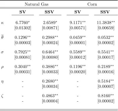
reasonable magnitude. Convergence is significant for all parameters at the 5 % or 10 % level according to the Geweke convergence test. We find a positive correlation between the natural gas (corn) futures price and the variance processes, ρ, of 0.30 and 0.39 (0.12 and 0.22) for theSV_{and the}SSV Model_{, respectively. This result}

is in line with Trolle and Schwartz (2010), who also observe a moderately positive correlation in the case of natural gas, although for a different time period. For corn, the correlation is also positive but lower with 0.12 and 0.22 for the SV _and

the SSV Model_{. When comparing the volatility parameters between natural gas}

and corn, it can be seen that the implied volatility for natural gas is far higher than the for corn. This matches the observations of historical volatility in the two markets.

For natural gas, the long-run mean of the variance process, θ, is lower for the SV Model _{than for the} SSV Model_{. Specifically, the estimated}_θ _{value for}

the SV Model _{corresponds to a long-run average volatility of 36 %. In the case}

of the SSV Model_{, the parameter estimates obtained translate into a minimum}

of 46.7 % and a maximum of 64 % for the time-varying seasonal long-run mean volatility. On the other hand, the vol-of-vol parameter, σ, is estimated higher for the SV Model_{, increasing the volatility of the variance process. Therefore, it}

seems that the error induced by ignoring the seasonal fluctuations of the variance levels is captured by a higher variability while inducing a downward bias in the long-term level estimate.

(22)

In the case of corn, θ corresponds to a long-run average volatility of 21.4 % for the SV Model _{while for the} SSV Model_{, the parameters imply a minimum}

of 19.7 % and a maximum of 27 %. The vol-of-vol parameter, σ, is also of similar magnitude for both model specifications.

The estimation result ofζ describes the shift of the seasonality function along the time-axis. The result for natural gas implies θ(t) to be the highest in late September and early October, while reaching a minimum in late March and early April. This result fits the empirical observations regarding a higher volatility during the fall and winter than during the summer months by, see, e.g., Suenaga et al. (2008) and Geman and Ohana (2009). The economic rationale for this pattern is the high sensitivity of natural gas prices to weather-related demand shocks during the winter since supply and demand are relatively price inelastic. The high values ofθ(t) during the fall pull up the volatility for natural gas, while in early spring, by the end of the cold season, the drift component brings the volatility down again. The opposite is true for corn, where the estimatedζvalue implies volatility reaching a high in June when information regarding the new harvest is being resolved while volatility during the winter months is much lower, see, e.g., Karali and Thurman (2010).

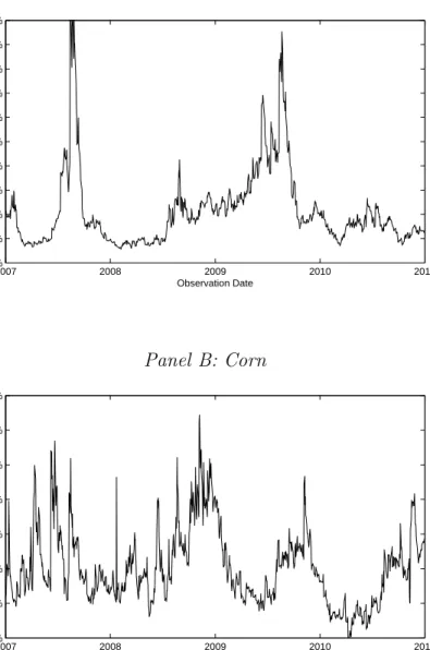
Figure 2 shows the paths obtained for the current volatility levels √Vt for

natural gas and corn during the time period considered for theSSV Model_{. Since}

(23)

√

Vt within both markets are very similar for the SV and SSV Models and

follow the same pattern over time. It becomes obvious that volatility of both natural gas as well as corn futures varies significantly over time. Additionally, it can be seen that during the considered time period, 2007 to 2010, realized

instantaneous volatility seems to be primarily driven by other factors like, e.g., the economic downturn and turbulences on the financial markets rather than by the normal seasonal demand cycle. However, for options pricing purposes, the market anticipated expected volatility is of relevance, not realized volatility. Yet, compared to other time periods with a more pronounced seasonal pattern, the relative performance of the SSV Model _{could potentially be downward biased}

and it will be interesting to see how the SSV Model _{performs in comparison to}

the SV Model _{in our study.}

B. Pricing Performance

Ultimately, we are interested in the pricing accuracy of an options valuation model. In particular, we want to see how the pricing ability of the SSV Model

incorporating a seasonal drift as the proposed model extension compares to the nested benchmark stochastic volatility model, the SV Model_.

As outlined before, the structural model parameters are estimated from the time series of futures prices from 1997 to 2006. Since this time period is chosen not to overlap with the 2007 to 2010 time period for our options pricing application,

(24)

no in-sample information is reflected in the structural parameters obtained which are estimated in the first step of our estimation approach. In the second step, the current variance level, Vt, and the variance risk premium, λ, are estimated

for each observation day t from the cross-section of observed option prices. Even though the SSV Model _{nests its non-seasonal counterpart and is therefore more}

flexible, the structural parameters are already determined at this point and only these two values,Vt and λ, are estimated from the options data – for both models.

In this sense, the models have the same degrees of freedom to fit observed option prices and the SSV Model _{will only yield a superior performance if the model}

extension picks up valuable information regarding the price dynamics in the first step of the estimation. Additionally, these price dynamics need to be persistent over time. Given the estimated parameters, we construct a time series of pricing errors according to different error metrics for the two models. Since Vt and λ are

estimated from the option contracts that are used to assess the pricing accuracy, we will refer to the pricing errors obtained as in-sample pricing errors.

To analyze the pricing accuracy of the two models, we report four different error metrics: The Root Mean Squared Error of Black (1976) implied volatilities,

IV-RMSE = q 1

Nt

PNt

i=1( ˆIVt,i−IVt,i)2, the Root Mean Squared Error of option

prices,$_-RMSE ₌q 1

Nt

PNt

i=1( ˆPt,i−Pt,i)2, the Relative Root Mean Squared Error,

RRM SE = q 1 Nt PNt i=1( ˆ Pt,i−Pt,i

Pt,i )2, and the Mean Percentage Error, M P E =

1 Nt PNt i=1 ˆ Pt,i−Pt,i

(25)

implied volatility of option i, ˆPt,i is the theoretical model price with implied

volatility ˆIVt,i, andNt is the number of observations at datet.

As Christoffersen and Jacobs (2004) point out, the most appropriate error metric to assess the performance of an options pricing model is the one employed as the loss function during the estimation. Hence, in this study, the IV-RMSE is the error metric which is at the center of interest. Additionally, we report the

$_{-RMSE and the RRMSE to assess the absolute and relative pricing errors and}

the MPE to look for systematic biases in the model prices obtained. All results are reported for the nine different maturity and moneyness brackets, as defined in Section III.

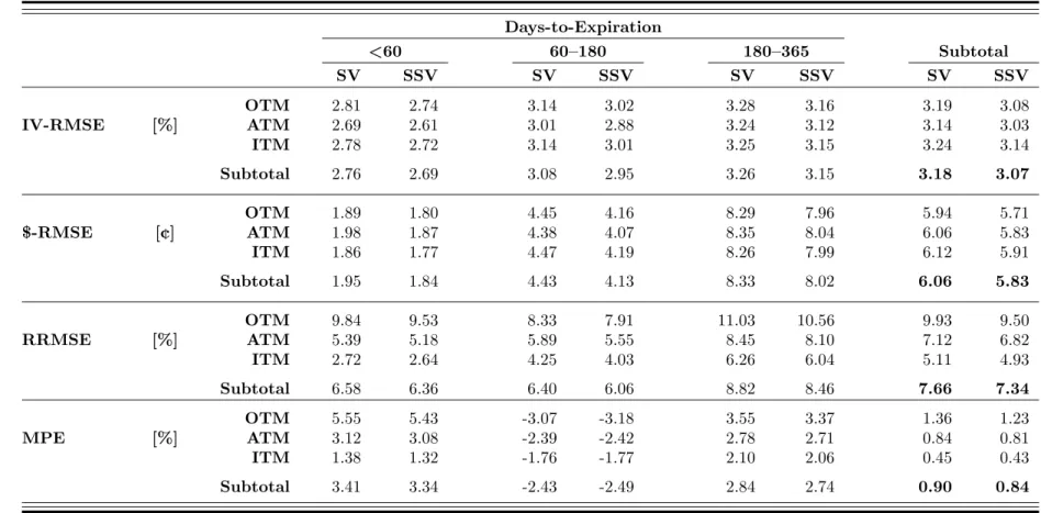
The in-sample results are provided in Tables 4 and 5 as average pricing errors according to the different metrics over the considered time period from January 3, 2007 to December 31, 2010 for natural gas and corn, respectively. In the case of natural gas, the resulting overall IV-RMSE is 3.18 % for the SV Model _and

3.07 % for the SSV Model_{. The overall} $_{-RMSE amounts to 6.06}¢ _{and 5.83}¢_,

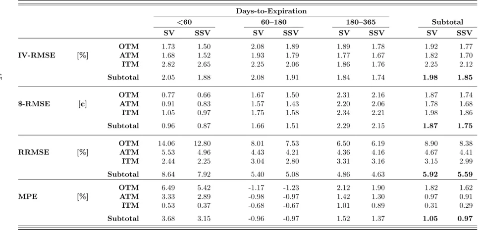
respectively, and the overall RRMSE is 7.66 % for theSV Model_{and 7.34 % for the} SSV Model_{. In the case of corn, the in-sample results can be summarized for the} SV _{and the} SSV Model _{as overall IV-RMSE being 1.98 % and 1.85 %,} $_-RMSE

being 1.87¢_{and 1.75}¢_{, and RRMSE being 5.92 % and 5.59 %. Not surprisingly, for}

both markets, the $_{-RMSE is higher for the more expensive long-term options and}

(26)

can be observed that mispricing is in every instance lower for the model including the seasonality component for natural gas as well as for corn. Furthermore, the MPE results reveal that on average both models tend to slightly overprice the options in both data sets. Particularly, for natural gas, the overall MPE is 0.90 % and 0.84 % for the SV _{and the} SSV Model_{, respectively, while the values for}

corn are 1.05 % and 0.97 %. Thereby, it is noteworthy that for both markets short-and long-term options are on average overpriced while medium-term options are on average underpriced.

To this point, it can be summarized that the SSV Model _{outperforms the} SV Model _{with respect to all four error metrics and for both markets being}

considered. More specifically, IV-RMSE, $_{-RMSE, and RRMSE are reduced not}

only overall but also for all moneyness and maturity brackets.

To see whether these results hold in a true out-of-sample case, we conduct the following analysis: For each day t, the current variance level Vt and the risk

premium λ are estimated with option price observations as in the previous case. These estimates are now used to price all options of the subsequent day, t + 1. Hence, no information from the day of the actual pricing comparison is utilized when calculating the theoretical option prices.

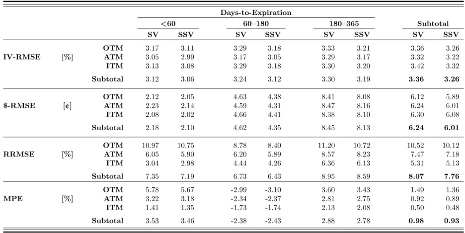
The out-of-sample results are summarized in Tables 6 and 7. Naturally, the average pricing errors obtained are somewhat higher than in the in-sample case. However, as in the in-sample study, it can be observed that the SSV Model

(27)

outperforms the SV Model _{for both markets and for all error metrics.} _In

particular for natural gas, the overall IV-RMSE is 3.36 % and 3.26 %, the$_-RMSE

is 6.24¢ _{and 6.01}¢_{, and the RRMSE is 8.07 % and 7.76 % for the} SV Model

and for the SSV Model_{, respectively. The corresponding results for corn are for}

IV-RMSE 2.51 % and 2.39 %, for$_{-RMSE 2.18}¢_{and 2.06}¢_{, and for RRMSE 7.09 %}

and 6.77 %.

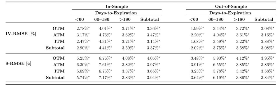
In a last step, we perform Wilcoxon signed-rank tests to inspect whether the observed differences in the pricing errors are also statistically significant. Specifically, the non-parametric Wilcoxon signed-rank test statistic tests whether the median of the differences is significantly different from zero. The percentage reductions in pricing errors in terms of IV-RMSE and $_{-RMSE are provided in}

Tables 8 and 9 for natural gas and corn, respectively. It can be observed that the pricing error reductions due to the proposed model extension are always significant at the 1 % level – for both markets, for every moneyness and maturity bracket, and for the in-sample as well as the out-of-sample study.

For natural gas, the inclusion of seasonality in the variance process reduces the in-sample (out-of-sample) IV-RMSE by 3.37 % (3.08 %) and the$_{-RMSE by 3.94 %}

(3.84 %). For corn, the reduction in terms of IV-RMSE yields 7.17 % (5.15 %) and in terms of $_{-RMSE 6.50 % (5.88 %). The greatest improvements can be observed}

for medium-term options: $_{-RMSE reductions for natural gas options amount to}

(28)

corn options. The observed pricing error improvements are not only statistically significant but can be considered economically significant as well.

Overall, we find clear empirical evidence that the proposed model extension of incorporating a seasonal component in the drift term of the variance process significantly improves the pricing accuracy for natural gas and corn options.

C. Comparison with Deterministic Volatility Model

In order to assess the influence of volatility being stochastic on the pricing performance, we compare the Seasonal Stochastic Volatility model to the Seasonal Deterministic Volatility (SDV) model of Back et al. (2013). In order to give the

SDV Model _{the highest chance to beat the} SSV Model_{, we recalibrate all}

parameters of the SDV model on a daily level, yielding the highest flexibility possible. We then use the parameters estimated on day t to price options on the following dayt+ 1. Table 10 reports the out-of-sample pricing errors for both markets (Panel A: Corn, Panel B: Natural Gas) when using implied volatilities for the calibration. Comparing these to the corresponding results in Table 6 and 7, we can observe that the pricing errors of theSDV Model_{are magnitudes higher than}

those of the SSV _(and SV₎ Model_{. The same is true for the in-sample results}

and when using pricing errors ($_{-RMSE) and not implied volatilities (IV-RMSE)}

as loss function in the calibration. The differences between theSDV _and SSV_are

(29)

We do not report these additional results in the spirit of brevity.20

D. Modeling Seasonal Volatility

In the main analysis of the paper, we have considered a relatively simple seasonal form for the variance process. A natural question is whether more complex seasonal forms can further improve the model’s performance. We have therefore added further trigonometric terms, in order to capture seasonal patterns at within year frequencies and have redone the analysis. Specifically, we have used the following specifications:

θ(t) =θ eη1sin(2π(t+ζ1))+η2sin(4π(t+ζ2)) ₍₁₇₎

θ(t) =θ eη1sin(2π(t+ζ1))+η2sin(4π(t+ζ2))+η3sin(8π(t+ζ3)) ₍₁₈₎

We denote the model with two seasonal components as SSV2 and the model with three seasonal components as SSV3. Results of this analysis are presented in Table 11 for natural gas and in Table 12 for corn.21 _{The upper panel in each table}

shows the comparison of SSV vs. SSV2, whereas the lower panel compares SSV2 vs. SSV3.

In the case of natural gas, we can observe that adding a second seasonal term pays off. Out-of-sample pricing errors are further reduced by about 5% which is

20

These results are available from the authors on request. 21

For the sake of brevity, we only report the reduction pricing errors when fitted to implied volatilities. All other tables lead to the same conclusions and are available on request.

(30)

also statistically significant. Adding a third component, however, has no longer any big impact. While we can observe a statistically significant reduction of the pricing errors, its economic effect is, with an improvement of 0.14%, hardly significant. In the case of corn options, we can observe that neither SSV2 nor SSV3 improve on SSV. In fact, all out-of-sample pricing errors are significantly larger (as indicated by negative reductions).

E. Further Robustness Checks

We conducted further robustness checks of our analysis. Due to space constraints, we refrain from presenting detailed results of these analyses, but summarize them below.

(i) In addition to utilizing IV-RMSE as objective function when estimating the current variance level Vt and the variance risk premium λ, we repeated our

analysis by applying the $_{-RMSE and the RRMSE as alternative loss functions.}

We found that the results obtained are robust with respect to these alternative loss functions. Furthermore, the observed pricing error reductions due to the model extension are all significant at the 1 % level and are of similar magnitude as for the primary loss functions. For natural gas, the overall out-of-sample IV-RMSE pricing error reduction is 3.16 % when using $_{-RMSE as objective function and}

3.33 % when applying RRMSE as objective function. For corn, the corresponding error reductions are 6.71 % and 5.82 %, respectively. Again, the improved pricing

(31)

performance is persistent across all moneyness and maturity brackets.

(ii) Since the structural model parameters, which are obtained out-of-sample under the physical measure from the historical futures prices, are different for the

SV_and SSV Model_{, the higher pricing accuracy of the seasonal volatility model}

might stem from the different parameter set and not from the seasonality extension. In order to control for this, we repeated the second step of the estimation procedure and obtained optimal Vt and λ values given the structural parameter values from

the SSV Model _{while restricting}_{η, the amplitude of the seasonality function, to}

be zero. We then compared the pricing accuracy of theSSV_andSV Models_when

having an identical set of structural parameters, with the only difference being that η is equal to zero for the SV Model_{. The results show that the pricing accuracy}

of the SV Model _{with these parameters is slightly improved for natural gas and}

slightly worse for corn. However, the results are unchanged: the SSV Model

consistently outperforms its non-seasonal counterpart in terms of both IV-RMSE and $_{-RMSE for every moneyness and maturity category, for both the in- and the}

out-of-sample study and for both markets. As before, all results are significant at the 1 % level.

V

Conclusion

Volatility in many commodity markets follows a pronounced seasonal pattern while also fluctuating stochastically. In this paper, we extend the stochastic volatility

(32)

model of Heston (1993) to allow volatility to vary with the seasonal cycle. The proposed model framework enables us to derive semi-closed-form solutions for pricing futures options. We then study the empirical performance in pricing natural gas and corn options. In contrast to other studies, we estimate our model using not only the cross-section of options prices but also considering the time series of futures contracts. The empirical results show that the suggested model indeed increases the accuracy of pricing natural gas and corn contracts, in terms of both statistical and economic significance.

Finally, we conclude the paper by outlining areas for further research. Many financial data exhibit jumps in prices and volatilities. This is also true for many commodity markets, and especially true for the natural gas market. Extending our model by including jump components is therefore a natural next step. Compared to equity markets in which the jump frequency is usually assumed to be constant, one might also consider modeling the jump intensity according to a seasonal function.

(33)

Appendix

For the practical application of any options pricing model, computational efficiency and robustness are of high importance. In order to facilitate the implementation, one can reformulate the valuation formula which was presented according to the standard terminology in Section II. For our empirical study, we employed the characteristic function formulation as proposed, e.g., by Albrecher et al. (2007) to overcome the branch cut problem with the original solution of Heston (1993).22 _{Furthermore, following the idea of Attari (2004), we rewrite the}

pricing formula in such a way that the ‘Heston-Integral’ in Equation (9) has to be evaluated only once instead of twice and that the integrand contains a square term in the denominator, causing the integral to converge faster. The obtained numerically more efficient formula for the price of a European call option on a futures contract is given by

C(F, K, V, T) = F e−r(T−t) − K 2e −r(T−t) +K πe −r(T−t) Z ∞ 0 Re f(φ) i [cos(φlnK)−isin(φlnK)] (φ−i)e−r(T−t)−φ−1 φ φ2₊₁ dφ. (19)

The characteristic function has the same form as before and the corresponding system of ODEs is given by

22

(34)

∂B ∂τ = 1 2σ 2_D2 −(κ+λ₋ρσφi)D₋ φi+φ 2 2 (20) ∂A ∂τ =κ θ(τ)D (21)

with τ =T ₋t. While Equation (21) has to be solved numerically,23 _{the solution}

of Equation (20) reads B(τ, φ) = κ+λ−ρσφi−d σ2 1₋e−dτ 1₋ge−dτ (22) with g =κ+λ−ρσφi−d κ+λ₋ρσφi+d (23) d=p(ρσφi₋κ₋λ)2₊_σ2_(φi₊_φ2_). ₍₂₄₎

Furthermore, the choice of the numerical integration procedure is of high importance for the implementation of any stochastic volatility model. Since the ODE in Equation (21) has to be solved for each evaluation within the numerical integration scheme of the ‘Heston-Integral’, this double integral is potentially computationally very costly. In contrast to adaptive methods like Gauss-Lobatto or the Simpson-Quadrature, a simple trapezoidal integration scheme brings the advantage that we can span a matrix with integral evaluations which can then be kept in memory and be called when needed for the next evaluation. Similar to the

23

For the SV Model_, _{the solution for Equation (21) is given by} _A₍_{τ, φ}₎ ₌

κθ σ2 h (κ+λ−ρσφi−d)τ−2 ln1₋ge−dτ 1₋g i .

(35)

caching technique of Kilin (2011), this approach dramatically reduces computing time for the option valuation in the proposed SSV Model_.

In particular, Kilin (2011) notes that the characteristic function is independent of the strike price and hence should be evaluated only once for each sub-sample of options having an equal time to maturity. Similarly, only the upper integration limit τ is different for each maturity sub-sample when solving the ODE in Equation (21). For a given grid of the ‘Heston-Integral’, all evaluations of this ODE up to the integration limit yield the same values and, hence, it is possible to evaluate this integral only once for the longest maturity Tmax and store the values

obtained in the computer’s memory. When evaluating the characteristic function for options with shorter maturities T, where T < Tmax, the necessary function

evaluations can be called from the stored values. Interpolation methods can be used if the matrix of stored values does not contain an evaluation corresponding exactly to the shorter maturity T. Hence, e.g., in our empirical study for natural gas with an average number of 365 options with 12 different maturity months for a given observation day, this yields 12 characteristic function evaluations for the SV Model_{and one additional numerical evaluation of the ODE in Equation (21) for}

the SSV Model_{. In this fashion, the proposed seasonal model extension can be}

(36)

References

C. A. Abanto-Valle, V. H. Lachos, and D. K. Dey. Bayesian estimation of a skew-student-t stochastic volatility model. Methodology and Computing in Applied Probability, 17:721–738, 2015.

H. Albrecher, P. Mayer, W. Schoutens, and J. Tistaert. The little Heston trap.

Wilmott Magazine, January:83–92, 2007.

R. W. Anderson. Some determinants of the volatility of futures prices. Journal of Futures Markets, 5:331–348, 1985.

M. Attari. Option pricing using Fourier transforms: A numerically efficient simplification. Working Paper, March 2004.

J. Back, M. Prokopczuk, and M. Rudolf. Seasonality and the valuation of commodity options. Journal of Banking and Finance, 37:273–290, 2013.

G. Bakshi, C. Cao, and Z. Chen. Empirical performance of alternative option pricing models. Journal of Finance, 52:2003–2049, 1997.

G. Barone-Adesi and R. E. Whaley. Efficient analytic approximation of American option values. Journal of Finance, 42:301–320, 1987.

D. Bates. Post-’87 crash fears in S&P 500 futures options.Journal of Econometrics, 94:181–238, 2000.

F. Black. The pricing of commodity contracts. Journal of Financial Economics, 3: 167–179, 1976.

M. J. Brennan and E. S. Schwartz. Evaluating natural resource investments.

Journal of Business, 58:135–157, 1985.

M. Broadie, M. Chernov, and M. Johannes. Model specification and risk premia: Evidence from futures options. Journal of Finance, 62:1453–1490, 2007.

´

A. Cartea and T. Williams. UK gas market: The market price of risk and applications to multiple interruptible supply contracts. Energy Economics, 30: 829–846, 2008.

J. Casassus and P. Collin-Dufresne. Stochastic convenience yield implied from commodity futures and interest rates. Journal of Finance, 60:2283–2331, 2005.

(37)

J. W. Choi and F. A. Longstaff. Pricing options on agricultural futures: An application of the constant elasticity of variance option pricing model. Journal of Futures Markets, 5:247–258, 1985.

P. Christoffersen and K. Jacobs. The importance of the loss function in option valuation. Journal of Financial Economics, 72:291–318, 2004.

J. C. Cox, J. E. Ingersoll, and S. A. Ross. A theory of the term structure of interest rates. Econometrica, 53:385–407, 1985.

J. S. Doran and E. I. Ronn. Computing the market price of volatility risk in the energy commodity markets. Journal of Banking & Finance, 32:2541–2552, 2008. A. Doshi, J. Frank, and A. Thavaneswaran. Seasonal volatility models. Journal of

Statistical Theory and Applications, 10:1–10, 2011.

D. Duffie, J. Pan, and K. Singleton. Transform analysis and asset pricing for affine jump-diffusions. Econometrica, 68:1343–1376, 2000.

B. Eraker. Do stock prices and volatility jump? Reconciling evidence from spot and option prices. Journal of Finance, 59:1367–1403, 2004.

B. Eraker, M. Johannes, and N. G. Polson. The impact of jumps in volatility and returns. Journal of Finance, 58:1269–1300, 2003.

H. Geman and V.-N. Nguyen. Soybean inventory and forward curve dynamics.

Management Science, 51:1076–1091, 2005.

H. Geman and S. Ohana. Forward curves, scarcity and price volatility in oil and natural gas markets. Energy Economics, 31:576–585, 2009.

S. Geman and D. Geman. Stochastic relaxation, Gibbs distributions and the Bayesian restoration of images. IEEE Transactions on Pattern Analysis and Machine Intelligence, 6:721–741, 1984.

R. Gibson and E. S. Schwartz. Stochastic convenience yield and the pricing of oil contingent claims. Journal of Finance, 45:959–976, 1990.

D. Heath, R. A. Jarrow, and A. Morton. Bond pricing and the term structure of interest rates: A new methodology for contingent claims valuation.

(38)

S. L. Heston. A closed-form solution for options with stochastic volatility with applications to bond and currency options. Review of Financial Studies, 6:327– 343, 1993.

E. Jacquier, N. G. Polson, and P. E. Rossi. Bayesian analysis of stochastic volatility models. Journal of Business and Economic Statistics, 12:371–389, 1994.

M. Johannes and N. G. Polson. MCMC methods for financial econometrics. In Y. A¨ıt-Sahalia and L. Hansen, editors, Handbook of Financial Econometrics. Elsevier, 2006.

B. Karali and W. N. Thurman. Components of grain futures price volatility.Journal of Agricultural and Resource Economics, 35:167–182, 2010.

N. Khoury and P. Yourougou. Determinants of agricultural futures price volatilities: Evidence from Winnipeg Commodity Exchange. Journal of Futures Markets, 13: 345–356, 1993.

F. Kilin. Accelerating the calibration of stochastic volatility models. Journal of Derivatives, 18:7–16, 2011.

P. Liu and K. Tang. The stochastic behavior of commodity prices with heteroskedasticity in the convenience yield. Journal of Empirical Finance, 18: 211–224, 2011.

R. Lord and C. Kahl. Complex logarithms in Heston-like models. Mathematical Finance, 20:671–694, 2010.

M. Manoliu and S. Tompaidis. Energy futures prices: Term structure models with Kalman filter estimation. Applied Mathematical Finance, 9:21–43, 2002.

J. Nakajima and Y. Omori. Stochastic volatility model with leverage and asymmetrically heavy-tailed error using gh skew student’s t-distribution.

Computational Statistics & Data Analysis, 56:3690–3704, 2012.

K. Ovararin and N. Meade. Mean reversion and seasonality in GARCH of agricultural commodities. International Conference On Applied Economics, 2010. M. Richter and C. Sørensen. Stochastic volatility and seasonality in commodity

(39)

B. R. Routledge, D. J. Seppi, and C. S. Spatt. Equilibrium forward curves for commodities. Journal of Finance, 55:1297–1338, 2000.

E. S. Schwartz. The stochastic behavior of commodity prices: Implications for valuation and hedging. Journal of Finance, 52:923–973, 1997.

E. S. Schwartz and J. E. Smith. Short-term variations and long-term dynamics in commodity prices. Management Science, 46:893–911, 2000.

C. Sørensen. Modeling seasonality in agricultural commodity futures. Journal of Futures Markets, 22:393–426, 2002.

H. Suenaga, A. Smith, and J. Williams. Volatility dynamics of NYMEX natural gas futures prices. Journal of Futures Markets, 28:438–463, 2008.

K. Tang and W. Xiong. Index investment and the financialization of commodities.

Financial Analysts Journal, 68(5):54–74, 2012.

A. B. Trolle and E. S. Schwartz. Unspanned stochastic volatility and the pricing of commodity derivatives. Review of Financial Studies, 22:4423–4461, 2009. A. B. Trolle and E. S. Schwartz. Variance risk premia in energy commodities.

(40)

Panel A: Natural Gas 1998 2000 2002 2004 2006 2008 2010 10% 20% 30% 40% 50% 60% 70% Observation Date Volatility Panel B: Corn 1998 2000 2002 2004 2006 2008 2010 5 % 10% 15% 20% 25% 30% 35% 40% 45% 50% Observation Date Volatility

Figure 1: Historical Volatility of Natural Gas and Corn Futures

This figure shows historical volatilities of natural gas and corn front-month futures from January 1997 to December 2010. The historical volatilities were derived by calculating the annualized standard deviation of the daily returns for each observation month. Prices are from Bloomberg.

(41)

Panel A: Natural Gas 2007 2008 2009 2010 2011 0% 20% 40% 60% 80% 100% 120% 140% 160% 180% 200% Observation Date Volatility Panel B: Corn 2007 2008 2009 2010 2011 0 % 10% 20% 30% 40% 50% 60% 70% Observation Date Volatility

Figure 2: Estimated Current Volatility Levels

This figure shows the current volatility level√Vtobtained during the considered time

period January 3, 2007 to December 31, 2010 for theSSV Model_{using the IV-RMSE}

criterion for the estimation from the cross-section of observed natural gas and corn futures option prices.

(42)

Table 1: Sample Description of Natural Gas Futures Options

This table shows average prices for the natural gas futures options grouped according to moneyness and time to maturity for both call and put options. The numbers of observations are reported in parentheses. Prices are obtained from Bloomberg for the period from January 1, 2007 to December 31, 2010.

Call Options Days-to-Expiration

S/K <60 60–180 180–365 Subtotal ITM 1.05–1.1 $0.7187 $ 1.0117 $1.2297 (6,105) (13,082) (15,920) (35,107) ATM 0.95–1.05 $0.4307 $ 0.7473 $0.9734 (16,687) (36,899) (41,978) (95,564) OTM 0.9–0.95 $0.2353 $ 0.5307 $0.7189 (10,040) (23,031) (23,259) (56,330) Subtotal (32,832) (73,012) (81,157) (187,001) Put Options ITM 0.9–0.95 $0.7447 $ 1.0240 $1.2107 (7,948) (17,564) (19,730) (45,242) ATM 0.95–1.05 $0.4347 $ 0.7147 $0.9369 (16,469) (35,320) (41,108) (92,897) OTM 1.05–1.1 $0.2173 $ 0.4774 $0.6949 (7,410) (16,183) (18,736) (42,329) Subtotal (31,827) (69,067) (79,574) (180,468) Total (64,659) (142,079) (160,731) (367,469)

(43)

Table 2: Sample Description of Corn Futures Options

This table shows average prices for the corn futures options grouped according to moneyness and time to maturity for both call and put options. The numbers of observations are reported in parentheses. Prices are obtained from Bloomberg for the period from January 1, 2007 to December 31, 2010.

Call Options Days-to-Expiration

S/K <60 60–180 180–365 Subtotal ITM 1.05–1.1 $ 0.3928 $ 0.5496 $ 0.6936 (2,132) (3,225) (4,426) (9,783) ATM 0.95–1.05 $ 0.2141 $ 0.3865 $ 0.5417 (5,295) (7,439) (11,032) (23,766) OTM 0.9–0.95 $ 0.0926 $ 0.2532 $ 0.4095 (2,796) (4,264) (6,479) (13,539) Subtotal (10,223) (14,928) (21,937) (47,088) Put Options ITM 0.9–0.95 $ 0.4475 $ 0.6185 $ 0.7627 (2,703) (4,141) (5,755) (12,599) ATM 0.95–1.05 $ 0.2240 $ 0.3966 $ 0.5418 (5,286) (7,413) (10,708) (23,407) OTM 1.05–1.1 $ 0.0867 $ 0.2306 $ 0.3726 (2,177) (3,242) (4,812) (10,231) Subtotal (10,166) (14,796) (21,275) (46,237) Total (20,389) (29,724) (43,212) (93,325)

(44)

Table 3: Physical Measure Parameter Estimates

This table provides MCMC estimates of model parameters using a continuous series of six-months futures prices from Januray 1997 to December 2006 (Natural Gas and Corn). Parameter estimates and standard errors [in brackets] are the mean and standard deviation of the posterior distributions. The estimation is based on 1,000,000 replications, the first

400,000 are discarded as burn-in. ∗ _{indicates significance at the 10% level and}∗∗ _{at the 5%}

level according to the Geweke convergence test.

Natural Gas Corn

SV SSV SV SSV κ 6.7760∗ _2.6589∗ _9.1171∗∗ _11.3838∗∗ [0.01302] [0.00871] [0.00571] [0.00659] θ 0.1296∗∗ _0.2988∗∗ _0.0459∗∗ _0.0532∗∗ [0.00003] [0.00024] [0.00001] [0.00002] σ 0.7925∗∗ _0.6464∗∗ _0.5589∗∗ _0.5541∗∗ [0.00081] [0.00080] [0.00012] [0.00017] ρ 0.3040∗∗ _0.3886∗∗ _0.1196∗∗ _0.2189∗∗ [0.00031] [0.00033] [0.00020] [0.00016] η - 0.2680∗∗ _- _0.5184∗∗ - [0.00034] - [0.00007] ζ - 0.4863∗∗ _- _0.8160∗∗ - [0.00004] - [0.00002]

(45)

Table 4: Natural Gas: In-Sample Pricing Errors

This table displays in-sample pricing errors of options on natural gas futures. Pricing errors are reported as root mean squared errors of the implied volatilities (IV-RMSE), root mean squared errors of option prices ($_{-RMSE), relative root mean squared errors (RRMSE), and mean percentage errors} (MPE) of option prices for the SV_{and the} SSV Model_{. The pricing errors reported are calculated as average values over the period from January 3,}

2007 to December 31, 2010. Pricing errors are grouped by maturity and moneyness of the options. The risk premium and the current volatility level are estimated with regard to the IV-RMSE criterion.

Days-to-Expiration <₆₀ _60–180 _180–365 _Subtotal SV SSV SV SSV SV SSV SV SSV IV-RMSE [%] OTM 2.81 2.74 3.14 3.02 3.28 3.16 3.19 3.08 ATM 2.69 2.61 3.01 2.88 3.24 3.12 3.14 3.03 ITM 2.78 2.72 3.14 3.01 3.25 3.15 3.24 3.14 Subtotal 2.76 2.69 3.08 2.95 3.26 3.15 3.18 3.07 $-RMSE [¢] OTM 1.89 1.80 4.45 4.16 8.29 7.96 5.94 5.71 ATM 1.98 1.87 4.38 4.07 8.35 8.04 6.06 5.83 ITM 1.86 1.77 4.47 4.19 8.26 7.99 6.12 5.91 Subtotal 1.95 1.84 4.43 4.13 8.33 8.02 6.06 5.83 RRMSE [%] OTM 9.84 9.53 8.33 7.91 11.03 10.56 9.93 9.50 ATM 5.39 5.18 5.89 5.55 8.45 8.10 7.12 6.82 ITM 2.72 2.64 4.25 4.03 6.26 6.04 5.11 4.93 Subtotal 6.58 6.36 6.40 6.06 8.82 8.46 7.66 7.34 MPE [%] OTM 5.55 5.43 -3.07 -3.18 3.55 3.37 1.36 1.23 ATM 3.12 3.08 -2.39 -2.42 2.78 2.71 0.84 0.81 ITM 1.38 1.32 -1.76 -1.77 2.10 2.06 0.45 0.43 44

(46)

Table 5: Corn: In-Sample Pricing Errors

This table displays in-sample pricing errors of options on corn futures. Pricing errors are reported as root mean squared errors of the implied volatilities (IV-RMSE), root mean squared errors of option prices ($_{-RMSE), relative root mean squared errors (RRMSE), and mean percentage errors (MPE)} of option prices for the SV _{and the} SSV Model_{. The pricing errors reported are calculated as average values over the period from January 3, 2007}

to December 31, 2010. Pricing errors are grouped by maturity and moneyness of the options. The risk premium and the current volatility level are estimated with regard to the IV-RMSE criterion.

(47)

Table 6: Natural Gas: Out-of-Sample Pricing Errors

This table displays out-of-sample pricing errors of options on natural gas futures. Pricing errors are reported as root mean squared errors of the implied volatilities (IV-RMSE), root mean squared errors of option prices ($_{-RMSE), relative root mean squared errors (RRMSE), and mean percentage errors} (MPE) of option prices for the SV_{and the} SSV Model_{. The pricing errors reported are calculated as average values over the period from January 4,}

2007 to December 31, 2010. Pricing errors are grouped by maturity and moneyness of the options. The risk premium and the current volatility level are estimated with regard to the IV-RMSE criterion. Theoretical model-based prices are derived by using parameters estimated the day before.

(48)

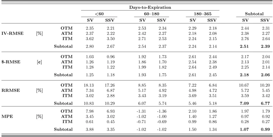
Table 7: Corn: Out-of-Sample Pricing Errors

This table displays out-of-sample pricing errors of options on corn futures. Pricing errors are reported as root mean squared errors of the implied volatilities (IV-RMSE), root mean squared errors of option prices ($_{-RMSE), relative root mean squared errors (RRMSE), and mean percentage errors} (MPE) of option prices for the SV_{and the} SSV Model_{. The pricing errors reported are calculated as average values over the period from January 4,}

2007 to December 31, 2010. Pricing errors are grouped by maturity and moneyness of the options. The risk premium and the current volatility level are estimated with regard to the IV-RMSE criterion. Theoretical model-based prices are derived by using parameters estimated the day before.