A galloping quadruped model using left-right asymmetry in touchdown angles.

Title

A galloping quadruped model using left-right asymmetry in

_{touchdown angles.}

Author(s)

Tanase, Masayasu; Ambe, Yuichi; Aoi, Shinya; Matsuno,

_Fumitoshi

Citation

Journal of biomechanics (2015), 48(12): 3383-3389

Issue Date

2015-09-18

URL

http://hdl.handle.net/2433/202761

Right

© 2015. This manuscript version is made available under the

CC-BY-NC-ND 4.0 license

http://creativecommons.org/licenses/by-nc-nd/4.0/; The

full-text file will be made open to the public on 18 September 2016

in accordance with publisher's 'Terms and Conditions for

Self-Archiving'.; この論文は出版社版でありません。引用の際

には出版社版をご確認ご利用ください。This is not the

published version. Please cite only the published version.

Type

Journal Article

A galloping quadruped model using left–right

asymmetry in touchdown angles

Masayasu Tanasea, Yuichi Ambea, Shinya Aoib,c,∗, Fumitoshi Matsunoa

a_{Dept. of Mechanical Engineering and Science, Graduate School of Engineering, Kyoto}

University, Kyoto Daigaku-Katsura, Nishikyo-ku, Kyoto 615-8540, Japan

b_{Dept. of Aeronautics and Astronautics, Graduate School of Engineering, Kyoto University,}

Kyoto Daigaku-Katsura, Nishikyo-ku, Kyoto 615-8540, Japan

c_{JST, CREST, 5 Sanbancho, Chiyoda-ku, Tokyo 102-0075, Japan}

Abstract

Among quadrupedal gaits, the galloping gait has specific characteristics in terms of locomotor behavior. In particular, it shows a left–right asymmetry in gait parameters such as touchdown angle and the relative phase of limb movements. In addition, asymmetric gait parameters show a characteristic dependence on locomotion speed. There are two types of galloping gaits in quadruped ani-mals: the transverse gallop, often observed in horses; and the rotary gallop, often observed in dogs and cheetahs. These two gaits have different footfall se-quences. Although these specific characteristics in quadrupedal galloping gaits have been observed and described in detail, the underlying mechanisms remain unclear. In this paper, we use a simple physical model with a rigid body and four massless springs and incorporate the left–right asymmetry of touchdown angles. Our simulation results show that our model produces stable galloping gaits for certain combinations of model parameters and explains these specific characteristics observed in the quadrupedal galloping gait. The results are then evaluated in comparison with the measured data of quadruped animals and the gait mechanisms are clarified from the viewpoint of dynamics, such as the roles of the left–right touchdown angle difference in the generation of galloping gaits and energy transfer during one gait cycle to produce two different galloping

∗_{Corresponding author}

gaits.

Keywords: Galloping gait, Quadruped, Model, Touchdown angle, Left–right

asymmetry, Center of mass movement, Energy transfer

1. Introduction 1

Quadruped animals use various gaits depending on the locomotion speed.

2

They use a walking gait in the lowest range of locomotion speed, and this

3

changes to a trotting gait as the locomotion speed increases. In the highest range

4

of locomotion speed, they use a galloping gait. These gaits are characterized by

5

footfall sequence [32]. During gaits used at slow speeds, such as a walking gait,

6

at least one limb is in contact with the ground, that is, in the stance phase. In

7

contrast, gaits used at higher speeds, such as a galloping gait, have a flight phase

8

during which all four limbs are in the air, that is, in the swing phase. These

9

gaits have been investigated from mechanical, energetic, kinematic, and kinetic

10

viewpoints to clarify the underlying mechanism for the use of such different gaits

11

depending on the locomotion speed [1, 13, 22, 23, 24, 31].

12

Among these quadrupedal gaits, the galloping gait has characteristic

prop-13

erties. Differing from the walking and trotting gaits, the galloping gait is

asym-14

metric [1, 22, 23]. More specifically, the relative phase of the movements between

15

the left and right limbs is away from the antiphase, unlike the walking and

trot-16

ting gaits, as shown in Fig. 1A. In addition, as the locomotion speed increases,

17

the relative phase decreases and approaches the in-phase as in a bounding gait,

18

which is not generally used by large, cursorial quadrupeds [26]. There are two

19

types of galloping gaits in quadruped animals, the transverse gallop and the

20

rotary gallop, and the two gaits have different footfall sequences (Fig. 1B) [22].

21

The transverse gallop is the preferred gait of horses, and the foot contacts take

22

place in the order of a hindlimb, the contralateral hindlimb, the ipsilateral

fore-23

limb, and the contralateral forelimb. The rotary gallop is the preferred gait of

24

dogs and cheetahs, and the foot contacts occur in the sequence of a hindlimb, the

0 0.2 0.4 0.6 0.8 0.1 0.3 1 3 10 30

Relative phase [rad]

Froude number Dog Sheep Camel Indian Rhinoceros White Rhinoceros Ferret Rat Jird Coypu Gallop Walk, Trot π π π π π

A

Transverse Gallop Rotary Gallop

B

TH (Left Hind) TF (Right Fore) LF (Left Fore) LH (Right Hind)

Figure 1: Characteristics of the quadrupedal galloping gait. A: relative phase between left and right forelimbs of quadrupeds depending on locomotion speed (Froude number), modified from [1]. Although it remains almost antiphase in the walking and trotting gaits, it is away from the antiphase and approaches the in-phase in the galloping gait as the locomotion speed increases. B: footfall diagrams of the transverse gallop of horses and the rotary gallop of dogs and cheetahs, modified from [22]. The transverse gallop has a single flight phase after the liftoff of the forelimbs, while the rotary gallop has two flight phases after the liftoff of the hindlimbs and forelimbs. TH: trailing hindlimb, TF: trailing forelimb, LH: leading hindlimb, and LF: leading forelimb.

contralateral hindlimb, the contralateral forelimb, and the ipsilateral forelimb.

26

Both gallops have a flight phase after the liftoff of the forelimbs. In contrast, the

27

fast rotary gallop of dogs and cheetahs has another flight phase after the liftoff

28

of the hindlimbs, unlike the transverse gallop of horses [5, 23] (some species

29

show a rotary gallop with just one flight phase at low speeds [25]). Although

30

these specific characteristics in quadrupedal galloping gaits and the dependence

31

on the locomotion speed and species have been observed and described in

de-32

tail [1, 5, 22, 23], the underlying dynamic mechanisms remain unclear.

33

Locomotion in humans and animals involves moving the center of mass

34

(COM) of the whole body using the limbs. The essential contribution of a

limb in locomotion dynamics can be represented by a spring. To explain the

36

locomotion mechanisms from a dynamic viewpoint, spring-loaded inverted

pen-37

dulum models have been used [6, 7, 8, 9, 11, 16, 29, 30, 36]. In particular,

38

for human running, the dependence of stability on touchdown angles has been

39

clarified [17, 19, 38]. A simple model having mass and two springs has been

40

used to explain the characteristic difference between human walking and

run-41

ning, which appears in the vertical ground reaction forces: a double-peaked

42

shape in human walking, and a single-peaked shape in human running [18]. For

43

quadrupedal locomotion, a rigid body with two springy legs has shown the

sta-44

bility characteristics of a bounding gait [10, 35]. The difference in the energy

45

levels between the trotting, bounding, and galloping gaits also has been

exam-46

ined [33]. Although simple physical models with leg springs have been used

47

for the quadrupedal galloping gait [21, 26, 28, 33, 40], they do not explain the

48

above-mentioned specific characteristics. In this paper, we use a simple

physi-49

cal model with a rigid body and four massless springs. The simulation results

50

show that our model produces stable galloping gaits for certain combinations of

51

model parameters, and explains these specific characteristics in the quadrupedal

52

galloping gait. The results are then evaluated in comparison with quadruped

53

animals and the gait mechanisms are discussed from the viewpoint of dynamics.

54

2. Materials and Methods 55

2.1. Physical model 56

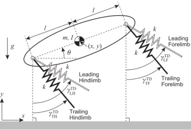
In this paper we use a physical model, which consists of a rigid body and

57

four massless springs in two dimensions (Fig. 2), as used in [33]. xand y are,

58

respectively, the horizontal and vertical positions of the COM of the body, and

59

θis the pitch angle. mandIare, respectively, the mass and moment of inertia

60

around the COM.lis the distance between the COM and the root of the spring.

61

g is the gravitational acceleration. +xis the locomotion direction. The front

62

two springs and the rear two springs represent the forelimbs and hindlimbs,

63

respectively. The spring constant isk. In the forelimbs, the anterior limb during

x y m, I l TF k k k k l θ (x, y) Leading Forelimb Trailing Forelimb γ LF γ LH γ TH γ Leading Hindlimb Trailing Hindlimb g TD TD TD TD

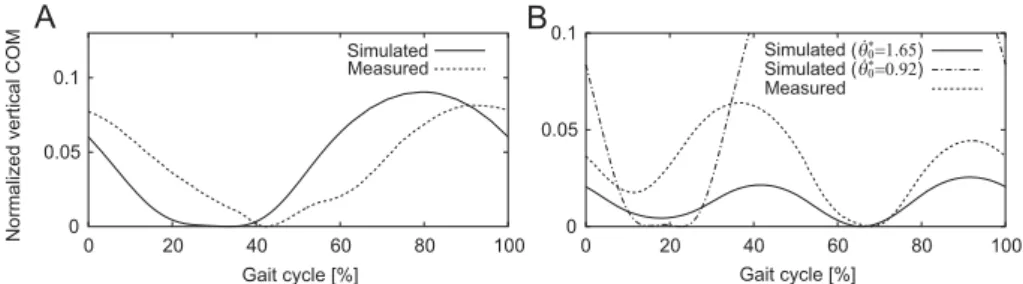
Figure 2: Physical model of galloping consisting of a rigid body and four massless springs in two dimensions.

the swing phase is the leading forelimb (LF) and the posterior limb is the trailing

65

forelimb (TF). Similarly, the anterior and posterior hindlimbs during the swing

66

phase are the leading hindlimb (LH) and trailing hindlimb (TH), respectively.

67

During the swing phase, the spring length remains the neutral lengthl₀and

68

the angle relative to the vertical line keeps the specific valueγ_iTD (i=LF, TF,

69

LH, TH), which corresponds to the touchdown angle (γ_LFTD≥γ_TFTD,γTD_LH ≥γ_THTD).

70

We assumed γ_LFTD+γ_TFTD ≥ 0 and γ_LHTD+γ_THTD ≥ 0 so that the trailing limbs

71

contact the ground earlier than the leading limbs, as observed in quadruped

72

animals. When a spring tip reaches the ground, it is constrained on the ground

73

and behaves as a frictionless pin joint. When the spring length returns to the

74

neutral length after the compression, the tip leaves the ground. Because the

75

touchdown and liftoff occur at the neutral length, this physical system is energy

76

conservative.

77

2.2. Governing equations 78

In our model, the four limbs have no influence on body dynamics during the

79

swing phase. In contrast, during the stance phase, they work as springs and

influence body dynamics through their compression. The motion of our model

81

is governed by the equations of motion ofx,y, andθ, which are given by

82 mx¨ = i=LF,TF,LH,TH −fisinγi my¨ = i=LF,TF,LH,TH ficosγi−mg Iθ¨ = i=LF,TF filcos(γi−θ)− i=LH,TH filcos(γi−θ) (1) where 83 fi = ⎧ ⎨ ⎩ −k(l_i−l₀) stance phase 0 swing phase

li and γi (i =LF, TF, LH, TH) are the spring length and the angle relative

84

to the vertical line, respectively, which are determined by x, y, θ, l, and the

85

touchdown position (l_i=l₀ andγ_i=γ_iTDduring the swing phase).

86

By using m, l₀, and l₀/g as the characteristic mass, length, and time

87

scale of our model, the state variables and parameters become dimensionless as

88

x∗ =x/l₀, y∗ =y/l₀, ˙()∗ = ˙()l₀/g, I∗ =I/(ml₀2), k∗ =kl₀/(mg),l∗ =l/l₀,

89

andl_i∗=l_i/l₀, which yields the dimensionless equations of (1) by

90 ¨ x∗ = i=LF,TF,LH,TH −f_i∗sinγi ¨ y∗ = i=LF,TF,LH,TH f_i∗cosγ_i−1 I∗θ¨∗ = i=LF,TF f_i∗l∗cos(γ_i−θ)− i=LH,TH f_i∗l∗cos(γ_i−θ) (2) where 91 f_i∗ = ⎧ ⎨ ⎩ −k∗(l_i∗−1) stance phase 0 swing phase

2.3. Generation of galloping gait using the left–right asymmetry of touchdown 92

angles 93

An important function of limbs in locomotion dynamics is to produce

trans-94

lational and rotational forces for the whole body through interaction with the

A

B

Figure 3: Different touchdown angles of (A) trailing and (B) leading hindlimbs in the horse galloping gait.

ground. Such forces are generated through the movements of the limb tip

rel-96

ative to the limb root (length and orientation). During a steady gait, the limb

97

tip produces a periodic trajectory relative to the body. When the relative phase

98

between the left and right limb movements is antiphase, as in walking and

trot-99

ting gaits, the left and right limbs move alternately relative to the body and

100

the periodic trajectories are almost identical between the left and right limbs.

101

When the relative phase is in-phase, as in a bounding gait, the left and right

102

limbs move simultaneously and the periodic trajectories are also almost

identi-103

cal between the left and right limbs. In contrast, during a galloping gait, the

104

relative phase is not in-phase or antiphase as shown in Fig. 1Aand the periodic

105

trajectories differ between the left and right limbs, which leads to the difference

106

in touchdown positions relative to the body as shown in Fig. 3 [21]. That is,

107

the touchdown angles are different between the left and right limbs.

108

In our model, when we use identical touchdown angles between the left

109

and right limbs (γ_LFTD =γ_TFTD, γ_LHTD=γ_THTD), foot contact occurs simultaneously

110

between the left and right limbs, which produces a bounding gait and a zero

111

relative phase between the left and right limbs. In contrast, different touchdown

112

angles (γ_LFTD = γ_TFTD, γ_LHTD = γ_THTD) induce different foot contact timings and

113

positions between the left and right limbs and yield a galloping gait. In addition,

114

an increase in the touchdown angle difference indicates an increase in the relative

phase between the left and right limbs.

116

2.4. Search of periodic solutions and stability analysis 117

We define the Poincar´e section when ˙y∗= 0 and when all four limbs are in the

118

swing phase (the model is in the flight phase). We find a periodic solution, which

119

corresponds to a gait, by searching for a fixed point in the Poincar´e section,

120

where we neglect x∗ because the horizontal position monotonically increases

121

during locomotion. In addition, we assume that all four limbs have to experience

122

the stance phase at least once before the intersection with the Poincar´e section so

123

that the solution explains a gait. When we setz∗= [y∗θx˙∗θ˙∗]T, the Poincar´e

124

mapP is written as

125

z_n∗₊₁=P(z_n∗, u∗) (3)

wherez_n∗ is the value ofz∗at thenth intersection with the Poincar´e section and

126

u∗ is the parameter set. When we denote ˆz∗for the fixed point on the Poincar´e

127

section, we obtain ˆz∗=P(ˆz∗, u∗).

128

In this paper, because the left–right touchdown angle differences are not

129

so different between the forelimbs and hindlimbs during galloping gaits [21],

130

we find gaits in which the differences in the left and right touchdown angles

131

are identical between the forelimbs and hindlimbs (γ_LFTD−γ_TFTD=γ_LHTD−γ_THTD).

132

In this condition, we can write the touchdown angles using the difference δ 133

(≥0) byγ_LFTD= ¯γ_FTD+δ/2,γ_TFTD= ¯γ_FTD−δ/2, γ_LHTD = ¯γ_HTD+δ/2, and γ_THTD =

134

¯

γTD_H −δ/2 (¯γ_FTD,γ¯_HTD ≥ 0), and the parameter set of this model is given by

135

u∗ = [I∗k∗l∗¯γ_FTDγ¯_HTDδ]T. We used the following four constraints: ˆy∗ =y∗₀,

136

ˆ

θ=θ0,ˆ˙θ∗= ˙θ₀∗, and F r=F r0, where F r is the Froude number defined by

137 F r= 1 τ∗ _τ∗ 0 x˙ ∗_dt∗ 2 (4) and τ∗ is a dimensionless one gait cycle [1]. We determined I∗ = 0.1 and

138

l∗= 0.6 based on the physical parameters of such quadruped animals as horses,

139

dogs, cheetahs, and goats [15, 20, 25, 39], and usedy₀∗ = 0.94 andθ₀ = 0.018.

140

To clarify the dynamic characteristics of galloping gait of our model, we used

various values fork∗, ˙θ∗₀, andF r₀and searched ˆ˙x∗, ¯γ_FTD, ¯γ_HTD, andδthat satisfy

142

ˆ

z∗=P(ˆz∗, u∗), where we used thefsolvefunction of MATLAB.

143

When we found periodic gaits, we investigated the local stability from the

144

eigenvalues of the linearized Poincar´e map around the fixed points. Because

145

our model is energy conservative, the gait is asymptotically stable when all

146

the eigenvalues except for one eigenvalue of 1 are inside the unit circle (these

147

magnitudes are less than 1).

148

3. Results 149

We obtained various periodic gaits depending on F r0, k∗, and ˙θ₀∗.

Fig-150

ures 4A and B show the angle difference δ for F r₀ and k∗ for the obtained

151

gaits with ˙θ∗₀ = 0.92 and 1.65, respectively. The gray regions show unstable

152

gaits and the white regions show stable gaits. The obtained gaits have different

153

sequences of the stance status (Sequences A–E), depending on the parameters,

154

as shown in Fig. 5. The obtained gaits in Fig. 4Ahave Sequences A–E, whereas

155

those in Fig. 4B have only Sequence E. Sequences B and E correspond to the

156

transverse and rotary gallops, respectively, in Fig. 1B. In both Figs. 4A and

157

B, as the locomotion speed increases, δ decreases and approaches 0 (but, did

158

not reach 0). At slow speeds (small Froude number), the obtained gaits are

159

unstable, and when the locomotion speed increases, the gaits become stable.

160

The dimensionless spring stiffness was estimated as 7 [14] or 12 [27] for horses,

161

11 [14] for dogs, and 16 [14] for goats. The left–right touchdown angle difference

162

during galloping gaits was observed around 5 to 15◦ [21]. The Froude number

163

of various quadruped animals is shown in Fig. 1Aand about 3 during the

trans-164

verse gallop of goats [14], and is seen to be greater than 50 during the rotary

165

galloping of cheetahs [5]. Our simulation results are comparable with biological

166

data.

167

To evaluate the biological relevance of the obtained gaits, we compared the

168

vertical COM movement of our simulation results with data measured during

169

quadrupedal galloping gaits. In Fig. 6A, we used ˙θ∗₀ = 0.92, F r₀ = 14.4,

0 10 20 30 40 50 4.5 5 5.5 1 2 3 4 5 6 7 8 Froude number Fr₀ Spring stiffness k∗ Angle difference [ ° ] A Seq. A Seq. B Seq. C Seq. D Seq. E 0 20 40 60 80 6 6.5 7 0 2 4 6 8 10 12 14 16 18 Froude number Fr₀ Spring stiffness k∗ B Seq. E δ

Figure 4: Touchdown angle differenceδof obtained gaits for Froude numberF r₀and spring stiffnessk∗ with (A) ˙θ₀∗= 0.92 and (B) ˙θ∗₀ = 1.65. Gray regions show unstable gaits, and white regions show stable gaits. Ahas five gaits (Sequences (Seqs.) A–E) depending onF r0 andk∗, whileB has one gait (Sequence E). Sequences A–E have different sequences of the stance condition, as shown in Fig. 5. The open dot (inA) and the black dots (inAandB) are the parameter sets used in Fig. 6 to compare vertical COM movement with the measured data for transverse and rotary gallops, respectively.

and k∗ = 5.1 (open dot in Fig. 4A) and compared the simulation result with

171

data measured during a transverse gallop by a horse (the Froude number is

172

around 18) [34]. The simulation result shows a single sinusoidal curve, and the

173

magnitude is similar to that of the measured data. The dimensionless spring

174

stiffness of a horse transverse gallop was estimated by 12 [27], and the simulation

175

result is fairly consistent with the measured data. In Fig. 6B, we used ˙θ₀∗= 0.92,

176

F r₀= 42.1, andk∗= 5.5 (black dot in Fig. 4A) and ˙θ∗₀= 1.65,F r₀= 25.7, and

177

k∗= 7.0 (black dot in Fig. 4B) and compared these simulation results with data

178

measured during a rotary gallop by a dog (the Froude number is about 20) [4].

179

The dimensionless spring stiffness of dogs was estimated by 11 [14]. When

180

˙

θ∗₀ = 0.92, the simulation result is very different in shape and magnitude from

181

the measured data. In contrast, for ˙θ∗₀= 1.65, although the magnitude is slightly

182

lower than the measured data, the simulation result shows a double sinusoidal

183

curve and has a similar shape to the measured data. This simulation result is

184

consistent with the measured data. See supplementary movies in Appendix A

185

for simulated locomotor behaviors.

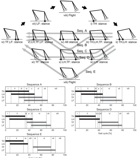
TF LF TF LF TF LF TF LF TF LF viii) Flight i) TH: stance ii) TH,LH: stance iv) All stance iii) TH,LH,TF: stance

v) LH,TF,LF: stance vi) TF,LF: stance vii) LF: stance ix) LH: stance x) LH,TF: stance xi) TF: stance viii) Flight 0 20 40 60 80 100 TH LH Sequence A 0 20 40 60 80 100 TH LH Sequence B 0 20 40 60 80 100 TH LH Sequence C 0 20 40 60 80 100 Gait cycle [%] TH LH Sequence D 0 20 40 60 80 100 Gait cycle [%] TH LH Sequence E Seq. A Seq. B Seq. C Seq. E Seq. D v x ix iv vi vii viii iii ii

i i ii iiix v vi vii viii

xi x vi vii viii ii i v vi vii viii ii i xi

viii vi vii viii ix

ii i

ix

Figure 5: Schematic sequences of stance condition of obtained gaits: Sequences (Seqs.) A–E. TH: trailing hindlimb, TF: trailing forelimb, LH: leading hindlimb, and LF: leading forelimb.

To clarify the dynamical difference between the obtained transverse and

187

rotary gallops, we investigated the energy transfer during one gait cycle.

Fig-188

ures 7AandBshow the ratio of four components of the conservative mechanical

189

energy (the gravitational energy (zero at the bottom of the vertical COM

move-190

ment), forelimb and hindlimb spring energies, and kinetic energy) for ˙θ₀∗= 0.92,

191

F r₀ = 14.4, and k∗ = 5.1 (transverse gallop), and ˙θ∗₀ = 1.65, F r₀ = 25.7, and

192

k∗= 7.0 (rotary gallop), respectively. In the transverse gallop, the gravitational

193

and kinetic energies move to the hindlimb spring energy during the first half

Normalized vertical COM

A

B

Figure 6: Comparison of vertical COM movement between the simulation results and measured data for one gait cycle between touchdowns of trailing hindlimbs during quadrupedal galloping gaits. A: transverse gallop using ˙θ₀∗= 0.92, F r0 = 14.4, andk∗= 5.1. Measured data are based on [34] from a horse. B: rotary gallop using ˙θ∗₀ = 0.92,F r₀= 42.1, andk∗= 5.5 and

˙

θ∗

0= 1.65,F r0= 25.7, andk∗= 7.0. Measured data are based on [4] from a dog.

of the hindlimb stance phase. The energy transitions into the kinetic energy

195

during the last half of the stance phase, and then changes to the forelimb spring

196

energy due to the touchdown of the forelimbs. Finally, it moves back to the

197

gravitational and kinetic energies. In the rotary gallop, the gravitational and

198

kinetic energies transition into the hindlimb spring energy during the first half

199

of the hindlimb stance phase, similarly to the transverse gallop. However, the

200

energy returns to the gravitational and kinetic energies during the last half of

201

the stance phase unlike the transverse gallop. The similar energy transfer occurs

202

in the forelimb stance phase. Although the rotary gallop has the energy transfer

203

to the gravitational energy between the hindlimb and forelimb stance phases,

204

the transverse gallop does not have such an energy transfer. This difference

205

produces two types of galloping gaits; the transverse gallop with a single flight

206

phase and the rotary gallop with two flight phases.

207

4. Discussion 208

In this paper, we produced galloping gaits using a simple model with a rigid

209

body and four massless springs, and showed that the model can explain specific

210

characteristics in a quadrupedal galloping gait, such as dependence of left–right

0 20 40 60 80 100 Ratio [%] Gait cycle [%] A B 98 99 100 0 20 40 60 80 100 Gait cycle [%] Kinetic Hindlimb Forelimb spring spring Gravitational 93 94 95 96 97 98 99 100 Hindlimb Forelimb spring spring Kinetic Gravitational

Figure 7: Energy transfer during one gait cycle for (A) transverse gallop using ˙θ∗₀ = 0.92,

F r0= 14.4, andk∗= 5.1 and (B) rotary gallop using ˙θ₀∗= 1.65,F r0= 25.7, andk∗= 7.0.

asymmetry in gait parameters on the locomotion speed, from the viewpoint of

212

dynamics.

213

4.1. Asymmetric gait parameters 214

In quadrupedal galloping gaits, the relative phase between the left and right

215

limbs is away from the antiphase, irrespective of species, as shown in Fig. 1A[1].

216

In addition, the relative phase decreases and approaches in-phase as the

loco-217

motion speed increases; however, it does not reach complete in-phase. These

218

characteristics reflect the left–right asymmetry in touchdown angles, as shown

219

in Fig. 3 [21]. We focused on this asymmetry to produce the galloping gait of

220

our model. As the locomotion speed increased, the left–right touchdown

an-221

gle difference decreased and approached 0 (but did not reach 0), as shown in

222

Fig. 4. This means that the relative phase difference decreased and approached

223

in-phase. This trend is consistent with the observations in quadrupedal

gallop-224

ing gaits. Furthermore, the fact that there is no solution for the zero left–right

225

touchdown angle difference means that this asymmetry in touchdown angles

226

allows the model to produce periodic solutions for gaits, which may suggest an

227

important role of left–right asymmetry in touchdown angles in the locomotion

228

dynamics of galloping gaits.

4.2. Transverse and rotary gallops 230

There are basically two types of galloping gaits (transverse and rotary

gal-231

lops) in quadruped animals, and they have different footfall sequences as shown

232

in Fig. 1B. The transverse gallop observed often in horses has a single flight

233

phase after the liftoff of the forelimbs. In contrast, the fast rotary gallop

ob-234

served often in dogs and cheetahs has another flight phase after the liftoff of

235

the hindlimbs in addition to the flight phase after the liftoff of the forelimbs.

236

Our simulation results showed that our model produced various galloping gaits

237

depending on the parameters, which had different sequences of the stance

condi-238

tion (Sequences A–E), as shown in Fig. 5. As locomotion speed and spring

stiff-239

ness increased, the sequence of the stance condition changed from Sequence A

240

to E. Sequences B and E corresponded to the transverse and rotary gallops,

241

respectively (because we cannot determine left and right limbs due to the

two-242

dimensional nature of our model, we decided these gaits from the number of

243

flight phases). However, even when the sequences of the stance condition were

244

identical, the locomotor behavior of the obtained gaits, such as the vertical COM

245

movement, differed depending on the parameters, as shown in Fig. 6. Depending

246

on the model parameters, both the sequences of stance condition and locomotor

247

behavior of the obtained gaits were comparable to those in quadruped animals,

248

which was evaluated by comparing our simulation results with measured data of

249

quadruped animals. Although quadruped animals use these two different gaits

250

depending on the locomotion speed and species, our simple model can explain

251

these different gaits using only a few parameters.

252

The transverse gallop has a small relative phase between the forelimbs and

253

hindlimbs, while the rotary gallop has a large relative phase, as shown in Fig. 1B.

254

In our simulation results, different parameters produced different relative phase

255

between the forelimbs and hindlimbs, as shown in Fig. 5, which changed the

256

number of flight phases and induced different galloping gaits. While the relative

257

phase between the left and right limbs depends on the left–right touchdown angle

258

differenceδ, our modeling has no constraint on the relative phase between the

259

forelimbs and hindlimbs, which were only determined through gait dynamics

with parameters. The dynamic mechanism that creates two different gaits was

261

ascertained from the energy transfer during one gait cycle in Fig. 7. It has

262

been suggested that horse transverse galloping and human skipping gaits have a

263

similarity in the energy transfer between the leading and trailing limbs [30]. We

264

also intend to investigate the mechanism by improving our model in the future.

265

4.3. Gait stability 266

Gait stability is an important factor in dynamic locomotion, as investigated

267

in humans [17, 19, 38] and quadrupeds [2, 3, 10, 12, 35, 37]. Our simulation

268

results showed that the galloping gait of our model was stable depending on the

269

Froude number (Fig. 4). That is, our model had self-stability for a particular

270

locomotion speed. More specifically, our model generated stable galloping gaits

271

only at fast locomotion speeds (F r₀ >5), which is consistent with the

obser-272

vation in quadrupedal galloping gaits as shown in Fig. 1A[1]. At slow speeds,

273

the obtained galloping gaits became unstable. This limitation of gait stability

274

due to the decrease in locomotion speed suggests a change of the gait to an

275

alternative gait, such as a trotting gait, to improve gait stability.

276

4.4. Limitation of our model and future work 277

In this study, we used a very simplified physical model for quadrupedal

gal-278

loping gaits. For example, the galloping quadruped animal was modeled by

279

a single rigid body and four massless springs, and symmetric assumptions

be-280

tween the forelimbs and hindlimbs were used in the model parameters, such

281

as the left–right touchdown angle difference δ and dimensionless spring

stiff-282

nessk∗. Such simplifications resulted in quantitative differences in locomotion

283

parameters from actual animals. However, it is clear that our model showed

284

similar trends in the asymmetric gait parameters for the locomotion speed

285

and in the generation of two different galloping gaits, which are

characteris-286

tic for quadrupedal galloping gaits, as was confirmed by the comparisons with

287

quadruped animals. This suggests that our simple model is capable of capturing

288

the essential aspects needed to generate the galloping gait in quadruped animals

from the viewpoint of dynamics. To further clarify the underlying mechanisms

290

in quadrupedal galloping gaits, we intend to develop a more sophisticated and

291

plausible model by incorporating important dynamical factors, such as

mus-292

cle actuators, frictional dissipation, and neuromechanical interactions, in future

293

studies.

294

Appendix A. Supplementary materials 295

We prepared two supplementary movies on the transverse and rotary gallops

296

obtained in our simulation:

297

1. Transverse gallop using ˙θ∗₀= 0.92,F r0= 14.4, andk∗= 5.1.

298

2. Rotary gallop using ˙θ∗₀= 1.65,F r₀= 25.7, andk∗= 7.0.

299

Acknowledgment 300

This paper was supported in part by JST, CREST.

301

Conflict of interest statement 302

The authors have no conflict of interests.

303

References 304

[1] Alexander, R.McN., and Jayes, A.S., 1983.A dynamic similarity hypothesis 305

for the gaits of quadrupedal mammals, J. Zool., Lond., 201:135–152.

306

[2] Aoi, S., Yamashita, T., and Tsuchiya, K., 2011.Hysteresis in the gait transi-307

tion of a quadruped investigated using simple body mechanical and oscillator 308

network models, Phys. Rev. E, 83(6):061909.

309

[3] Aoi, S., Katayama, D., Fujiki, S., Tomita, N., Funato, T., Yamashita, T.,

310

Senda, K., and Tsuchiya, K., 2013.A stability-based mechanism for hystere-311

sis in the walk–trot transition in quadruped locomotion, J. R. Soc. Interface,

312

10(81):20120908.

[4] Bertram, J.E.A. and Gutmann, A., 2009. Motions of the running horse 314

and cheetah revisited: fundamental mechanics of the transverse and rotary 315

gallop, J. R. Soc. Interface, 6:549–559.

316

[5] Biancardi, C.M. and Minetti, A.E., 2012. Biomechanical determinants of 317

transverse and rotary gallop in cursorial mammals, J. Exp. Biol., 215:4144–

318

4156.

319

[6] Blickhan, R., 1989. The spring–mass model for running and hopping, J.

320

Biomech., 22:1217–1227.

321

[7] Bullimore, S.R. and Burn, J.F., 2006. Dynamically similar locomotion in 322

horses, J. Exp. Biol., 209:455-465.

323

[8] Bullimore, S.R. and Burn, J.F., 2006.Consequences of forward translation 324

of the point of force application for the mechanics of running, J. Theor.

325

Biol., 238:211-219.

326

[9] Bullimore, S.R. and Burn, J.F., 2007. Ability of the planar spring-mass 327

model to predict mechanical parameters in running humans, J. Theor. Biol.,

328

248:686-695.

329

[10] Cao, Q. and Poulakakis, I., 2013.Quadrupedal bounding with a segmented 330

flexible torso: passive stability and feedback control, Bioinspir. Biomim.,

331

8:046007.

332

[11] Cavagna, G.A., Heglund, N.C., and Taylor, C.R., 1977. Mechanical work 333

in terrestrial locomotion: two basic mechanisms for minimizing energy ex-334

penditure, Am. J. Physiol., 233(5):R243–R261.

335

[12] Diedrich, F.J. and Warren Jr., W.H., 1998.Why change gaits? Dynamics of 336

the walk-run transition, J. Exp. Psychol. Hum. Percept. Perform., 21:183–

337

202.

338

[13] Farley, C.T. and Taylor, C.R., 1991.A mechanical trigger for the trot-gallop 339

transition in horses, Science, 253:306–308.

[14] Farley, C.T., Glasheen, J., and McMahon, T.A., 1993. Running springs: 341

Speed and animal size, J. Exp. Biol., 185:71–86.

342

[15] Fischer, M.S., Lilje, K.E., Laustr¨oer, J., and Andikfar, A., 2011. Dogs in

343

motion,Dortmund: VDH-Service GmbH.

344

[16] Full, R.J. and Koditschek, D.E., 1999. Templates and anchors: neurome-345

chanical hypotheses of legged locomotion on land, J. Exp. Biol., 202:3325–

346

3332.

347

[17] Geyer, H., Seyfarth, A., and Blickhan, R., 2005.Spring-mass running: sim-348

ple approximate solution and application to gait stability, J. Theor. Biol.,

349

232:315–328.

350

[18] Geyer H., Seyfarth, A., and Blickhan, R., 2006. Compliant leg behaviour 351

explains basic dynamics of walking and running, Proc. R. Soc. B, 273:2861–

352

2867.

353

[19] Ghigliazza, R.M., Altendorfer, R., Holmes, P., and Koditschek, D., 2003.A 354

simply stabilized running model, SIAM J. Appl. Dyn. Syst., 2(2):187–218.

355

[20] Grossi, B. and Canals, M., 2010.Comparison of the morphology of the limbs 356

of juvenile and adult horses (Equus caballus) and their implications on the 357

locomotor biomechanics, J. Exp. Zool., 313A:292–300.

358

[21] Herr, H.M. and McMahon, T.A., 2001. A galloping horse model, Int. J.

359

Robot. Res., 20(1):26–37.

360

[22] Hildebrand, M., 1977. Analysis of asymmetrical gaits, J. Mammal.,

361

58(2):131–156.

362

[23] Hildebrand, M., 1989. The quadrupedal gaits of vertebrates, BioScience,

363

39(11):766–775.

364

[24] Hoyt, D.F. and Taylor, C.R., 1981.Gait and the energetics of locomotion 365

in horses, Nature, 292:239–240.

[25] Hudson, P.E., Corr, S.A., and Wilson, A.M., 2012. High speed galloping 367

in the cheetah (Acinonyx jubatus) and the racing greyhound (Canis famil-368

iaris): spatio-temporal and kinetic characteristics, J. Exp. Biol., 215:2425–

369

2434.

370

[26] Marhefka, D.W., Orin, D.E., Schmiedeler, J.P., and Waldron, K.J., 2003.

371

Intelligent control of quadruped gallops, IEEE/ASME Trans. Mechatron.,

372

8(4):446–456.

373

[27] McGuigan, M.P. and Wilson, A.M., 2003. The effect of gait and digital 374

flexor muscle activation on limb compliance in the forelimb of the horse 375

Equus caballus, J. Exp. Biol., 206:1325–1336.

376

[28] McMahon, T.A., 1985.The role of compliance in mammalian running gaits,

377

J. Exp. Biol., 115:263–282.

378

[29] McMahon, T.A. and Cheng, G.C., 1990.The mechanics of running: how 379

does stiffness couple with speed?, J. Biomech., 23(Suppl. 1):65–78.

380

[30] Minetti, A.E., 1998.The biomechanics of skipping gaits: a third locomotion 381

paradigm?, Proc. R. Soc. Lond. B, 265:1227–1235.

382

[31] Minetti, A.E., Ardigo, L.P., Reinach, E., and Saibene, F., 1999.The rela-383

tionship between mechanical work and energy expenditure of locomotion in 384

horses, J. Exp. Biol., 202:2329–2338.

385

[32] Muybridge, E., 1957. Animals in motion,New York: Dover Publications.

386

[33] Nanua, P. and Waldron, K., 1995.Energy comparison between trot, bound, 387

and gallop using a simple model, ASME J. Biomech. Eng., 117:466–473.

388

[34] Pfau, T., Witte, T.H., and Wilson, A.M., 2006.Centre of mass movement 389

and mechanical energy fluctuation during gallop locomotion in the Thor-390

oughbred racehorse, J. Exp. Biol., 209:3742–3757.

[35] Poulakakis, I., Papadopoulos, E., and Buehler, M., 2006. On the stability 392

of the passive dynamics of quadrupedal running with a bounding gait, Int.

393

J. Robot. Res., 25(7):669–687.

394

[36] Raibert, M.H., 1986. Legged robots that balance,Cambridge: MIT Press.

395

[37] Sch¨oner, G., Jiang, W.Y., and Kelso, J.A.S., 1990. A synergetic theory of 396

quadrupedal gaits and gait transitions, J. Theor. Biol., 142:359–391.

397

[38] Seyfarth, A., Geyer, H., G¨unther, M., and Blickhan, R., 2002.A movement 398

criterion for running, J. Biomech., 35:649–655.

399

[39] Taylor, C.R., Shkolnik, A., Dmi’el, R., Baharav, D., and Borut, A., 1974.

400

Running in cheetahs, gazelles, and goats: energy cost and limb conjguration,

401

Am. J. Physiol., 227(4):848–850.

402

[40] Waldron, K., Estremera, J., Csonka, P., and Singh, S., 2009. Analyz-403

ing bounding and galloping using simple models, ASME J. Mech. Rob.,

404

1(1):011002.