Copyright belongs to the author. Small sections of the text, not exceeding three paragraphs, can be used provided proper acknowledgement is given.
The Rimini Centre for Economic Analysis (RCEA) was established in March 2007. RCEA is a private, nonprofit organization dedicated to independent research in Applied and Theoretical Economics and related fields. RCEA organizes seminars and workshops, sponsors a general interest journal The Review of Economic Analysis, and organizes a biennial conference: The Rimini Conference in Economics and Finance (RCEF). The RCEA has a Canadian branch: The Rimini Centre for Economic Analysis in Canada (RCEA-Canada). Scientific work contributed by the RCEA Scholars is published in the RCEA Working Papers and Professional Report series.
The views expressed in this paper are those of the authors. No responsibility for them should be attributed to the Rimini Centre for Economic Analysis.
The Rimini Centre for Economic Analysis
Legal address: Via Angherà, 22 – Head office: Via Patara, 3 - 47900 Rimini (RN) – Italy www.rcfea.org - [email protected]
WP 11-09
Gary Koop
University of Strathclyde
The Rimini Centre for Economic Analysis (RCEA)
Roberto Leon-Gonzalez
National Graduate Institute for Policy Studies
The Rimini Centre for Economic Analysis (RCEA)
Rodney Strachan
The Australian National University
B
AYESIAN
M
ODEL
A
VERAGING IN THE
I
NSTRUMENTAL
V
ARIABLE
R
EGRESSION
Bayesian Model Averaging in the
Instrumental Variable Regression Model
Gary Koop
University of Strathclyde
Roberto Leon-Gonzalez
National Graduate Institute for Policy Studies
Rodney Strachan
The Australian National University
January 2011
All authors are fellows of the Rimini Centre for Economic Analysis. The authors would like to thank Frank Kleibergen and other partipants at the European Seminar on Bayesian Econometrics for helpful comments as well as the Leverhulme Trust for …nancial support under Grant F/00 273/J. Leon-Gonzalez also thanks the Japan Society for the Promotion of Science for …nancial support (start-up Grant #20830025). Corresponding author: Roberto Leon-Gonzalez, [email protected].
ABSTRACT
This paper considers the instrumental variable regression model when there is uncertainty about the set of instruments, exogeneity restrictions, the validity of identifying restrictions and the set of exogenous regressors. This uncertainty can result in a huge number of models. To avoid statistical problems associated with standard model selection procedures, we develop a reversible jump Markov chain Monte Carlo algorithm that allows us to do Bayesian model averaging. The algorithm is very ‡exible and can be easily adapted to analyze any of the di¤erent priors that have been proposed in the Bayesian instrumental variables literature. We show how to calculate the probability of any relevant restriction (e.g. the posterior probability that over-identifying restrictions hold) and discuss diagnostic checking using the posterior distribution of discrepancy vectors. We illustrate our methods in a returns-to-schooling application.
Keywords:
Bayesian, endogeneity, simultaneous equations, reversible jump Markov chain Monte Carlo.1
Introduction
For the regression model where all potential regressors are exogenous, a large literature1 has arisen to address the problems caused by a huge model space. That is, the number of models under consideration is typically 2K whereK is the number of potential regressors. With such a huge model space, there are many problems with conventional model selection procedures (e.g. sequential hypothesis testing procedures run into pre-test problems). Bayesian model averaging (BMA) can be used to avoid some of these problems. However, the size of the model space means that carrying out BMA by estimating every model is typically computationally infeasible. Accordingly, an algo-rithm which simulates from the model space (e.g. the Markov chain Monte Carlo model composition algorithm of Madigan and York, 1995) must be used. In the case of the regression model with exogenous regressors, such methods are well-developed, well-understood and are increasingly making their way into empirical work. However, to our knowledge, there are no comparable papers for the empirically important case where regressors are potentially endogenous and, thus, instrumental variable (IV) methods are required.2 The purpose of the present paper is to …ll this gap.
Inference about structural parameters in the IV regression model requires the formulation of assumptions whose validity is often uncertain. A useful representation of the model is the incomplete simultaneous equations model (see, for example, Hausman, 1983). Within this representation, the most cru-cial assumptions relate to the set of instruments and the rank condition for identi…cation (Greene, 2003, p. 392). In addition to these, one has to decide how many regressors to include, and which of these are potentially endoge-nous. This can lead to a huge model space and, thus, similar issues arise as for the regression model with exogenous regressors. In practice, researchers typically try di¤erent speci…cations until a set of restrictions (i.e. a particular choice of instruments, exogenous and endogenous regressors) passes a battery of misspeci…cation tests (e.g. Anderson and Rubin, 1949, 1950, Hausman,
1See, among many others, Fernandez, Ley and Steel, 2001 and the references cited
therein.
2Two related papers are Cohen-Cole, Durlauf, Fagan, and Nagin (2009) and Eicher,
Lenkoski and Raftery (2009) but the model space in these papers is small and, hence, simulation methods from the model space are not required. Furthermore, the approach of these papers (averaging of two-staged least squares estimates using BIC-based weights) does not have a formal Bayesian justi…cation.
1983, Sargan, 1958). Given the large number of possible models, the re-peated application of diagnostic tests will result in similar distorted size and power properties as arise in the regression model with exogenous regressors. Since estimates of structural estimates that rely on incorrect identi…cation restrictions can result in large biases, the consequences of these problems can be substantive. BMA can be used to mitigate such problems. But the size of the model space often precludes estimation of all models. This leads to a need for computational methods which simulate from the model space. A contribution of the present paper is to design a reversible jump Markov chain Monte Carlo algorithm (RJMCMC, see Green, 1995 or Waagepetersen and Sorensen, 2001) that explores the joint posterior distribution of para-meters and models and thus allows us to do BMA. This allows us to carry out inference on the structural parameters that, conditional on identi…cation holding, accounts for model uncertainty. Furthermore, our algorithm allows for immediate calculation of the posterior probability associated with any restriction, model or set of models. Thus, we can easily check the validity of identifying restrictions (or exogeneity restrictions, etc.) by calculating the posterior probability of these restrictions. Alternatively, we can use the BMA posterior distribution of discrepancy vectors and functions (Zellner, Bauwens and van Dijk, 1988) in order to shed light on the validity of instruments.
In our applications, we …nd that standard versions of RJMCMC algo-rithms (e.g. adapting the RJMCMC methods for seemingly related regres-sion, SUR, models developed by Holmes, Denison and Mallick, 2002, to the IV case) can perform poorly, remaining stuck for long periods in models with low posterior probability. To improve the performance of our RJMCMC al-gorithms, we borrow an idea from the simulated tempering literature and augment our model space with so-called cold models. The cold models are similar to the models of interest (called hot models) but are simpli…ed in such a way that the RJMCMC algorithm makes very rapid transitions be-tween cold models. As suggested by the simulated tempering literature, we …nd that this strategy helps the algorithm escape from local modes in the posterior.
The RJMCMC algorithm we propose is very ‡exible and can be easily adapted to handle any of the popular approaches to Bayesian inference in IV models. To illustrate this, we describe in detail how the algorithm works in the context of three popular Bayesian approaches to instrumental variables and reduced rank regression. These are the classic approach of Drèze (1976) as well as the modern approaches of Kleibergen and van Dijk (1998) and
Strachan and Inder (2004)3. We also show how, if desired, the RJMCMC algorithm can be easily coded to produce results for all three (or more) priors by running the algorithm just once.
Section 2 describes the model space we consider. Section 3 describes the algorithm with complete details being included in a Technical Appendix. Section 4 explains how to obtain the BMA posterior distribution of discrep-ancy measures for model diagnostics proposed by Zellner, Bauwens and van Dijk (1988). Section 5 applies our methods to a returns-to-schooling example based on Card (1995) and Section 6 concludes.
2
Modelling Choices in the Incomplete
Si-multaneous Equations Model
We will work with the incomplete simultaneous equations model, which takes the form:
y1i = 0y2i+ 0xi+u1i (1)
y2i = 2xxi+ 2zzi+v2i
wherey1i : 1 1, y2i :m 1, xi :k1j 1, zi :k2j 1,i= 1; :::; N. The errors
are normal with zero means and are uncorrelated over i. We assume
E xi u1i v2i 0 = 0 and E zi u1i v2i 0 = 0:
The reduced form version of this model can be written as:
yi = xxi+ zzi+vi (2)
3We use a proper prior version of the improper prior used by Drèze (1976), as in
the subsequent papers of Drèze and Richard (1983) and Zellner, Bauwens and van Dijk (1988). With respect to the prior by Strachan and Inder (2004), we will use a parameter-augmented version of it similar to that used by Koop, Leon-Gonzalez and Strachan (2010).
where yi = (y1i; y20i)0, vi = (v1i; v20i)0 and: x = 1x 2x = 0 2x+ 0 2x ; z = 1z 2z = 0 Im 2z = E(vivi0) =E u1i v2i u1i v02i = 11 12 21 22 = !11 !12 !21 22 = 1 0 0 Im 1 0 Im x : (m+ 1) k1j z : (m+ 1) k2j
The subindexj stands for the jth model, andj varies from1toNmod, where
Nmod is the total number of models. To avoid notational clutter, we will not attach j subindices to parameter matrices although, of course, these will vary over models.
When using this model, there are many sources of uncertainty over iden-ti…cation that arise. Assuming 12 6= 0; we can solve for the parameters
( 0; 0) from the reduced form matrix
e = [ x z]
through the relations
1x 0 2x = 0 and (3)
1z 0 2z = 0: (4)
If we are able to solve (4) for ; we can subsequently solve for using (3). Solving for depends upon the rank of the matrix z: If k2j = m and
rank( z) = mthen there is a unique solution 0 = 1z 2z1 and the equation
is just identi…ed. If k2j > m and rank( z) = m then there are many
solutions such as 0 =
1z 20z( 2z 20z)
1
where 2z is constructed from any set ofk mlinearly independent columns of 2z:In this case, the equation
is over-identi…ed. If k2j < m then rank( z) < m, so there are no solutions
and the equation is under-identi…ed.
Uncertainty over identi…cation can also result from uncertainty over what variables in y2i are endogenous and what variables in zi are not valid
in-struments. If we relax the earlier assumption on 12 to allow for 12 = 0;
which implies y2i is exogenous, then we have additional solutions for from
0 =!
determining whether( 0; 0)is just or over-identi…ed. A further complication
arises if elements of or 12 are zero as these restrictions imply elements of
y2i are exogenous. This e¤ectively changes the value of m, increasing the
number of identifying restrictions in (4) and, hence, the conditions for un-der, just and over identi…cation. Note also that, if k2i > m and rows of the
k2i m matrix 2z are zero, or, more generally, if rank( 2z) = mi < m,
then not all elements ofzi may be regarded as valid instruments. In this case,
we can then represent 2z as the product of two lower dimensional matrices,
2z = 2z% where 2z is m mi and % is mi k2i both full rank. The valid
instruments are then %zi:
Furthermore, if elements of are zero, then this gives us more equa-tions of the type (4) and few equaequa-tions of the type (3), again a¤ecting the identi…cation status of ( 0; 0).
In this paper, we consider a model space which includes all the over-identi…ed and just-over-identi…ed models (see below for a discussion of non-over-identi…ed models). These are the models in whichk2j mand 2z has full rank.
Mod-els in this category di¤er according to the following aspects:
Set of instruments: The variables inzi are a subset of a larger group of
potential instruments denoted byZ . There is uncertainty as to which subset of Z should enter in the model and hence uncertainty about the column dimension of the matrix 2z.
Variables in xi: xi is a subset of Z [X , where X is the set of all
potential regressors that are not allowed to be instruments. Uncertainty about what variables enter xi implies uncertainty over the elements of
:
Restrictions on the coe¢ cients of endogenous regressors: some coe¢ -cients in might be restricted to be zero.
Exogeneity: some of the covariances betweenu1i andv2i might be zero;
that is, there is uncertainty about the elements of 12.
Note that researchers typically have some exogenous variables that they are certain cannot be instruments (and thus, we introduce X as above). However, they are typically interested in checking the validity of all exclusion restrictions (i.e. restrictions that instruments do not enter the structural equation) and, for this reason, our set of potential exogenous regressors in
our equation of interest will include all the potential instruments (i.e. we
have xi Z [X ).
Note that just-identi…ed models are observationally equivalent to (non-identi…ed) full rank models (i.e. models where z has full rank) in which all
exclusion restrictions fail. In this sense we are also including non-identi…ed full rank models in our analysis. A problem arises in that di¤erent just-identi…ed models will all yield the same full rank model and, thus, are obser-vationally equivalent. That is, full rank models take the form of unrestricted SUR models. But di¤erent just-identi…ed models will always have the same unrestricted SUR reduced form (and, thus, yield the same marginal likeli-hood and be observationally equivalent). Over-identi…ed models will impose restrictions on the coe¢ cients in the reduced form SUR and break this obser-vational equivalence problem. But the obserobser-vational equivalence of di¤erent just-identi…ed models raises the question of how they should be included in a BMA exercise. As an example, consider a reduced form unrestricted SUR model with two equations and two explanatory variables, z1 and z2. This
reduced form is consistent with a just-identi…ed model where z1 is the
sin-gle valid instrument for the …rst equation. But it is also consistent with a just-identi…ed model wherez2 is the single valid instrument. Should we treat
these as two di¤erent models weighted equally when doing model averag-ing? This is a possible strategy that could be done. Or one might prefer to simply treat the two models as one model. Furthermore, as the identifying assumption cannot be tested in the just-identi…ed case, one might decide not to use just-identi…ed models when constructing BMA estimates of structural parameters. But of course just-identi…ed models could be included if desired, and this is what we do in our empirical analysis.
If some elements in (and/or ) are restricted to be zero then this increases the degree of over-identi…cation such that some models with k2j
m may, by these restrictions, become over-identi…ed. However, all of our over-identi…ed models have k2j > m. This condition is necessary because a
model with some zero restrictions on and with fewer than m instruments (even though its parameters are identi…ed) is observationally equivalent to a model in which all elements of are di¤erent from zero but 2z has reduced
rank. Thus, we consider over-identi…ed models to be those with k2j > m,
regardless of the restrictions on or .
In a subsequent section, we present empirical work based on the classic returns-to-schooling paper of Card (1995) and associated data set. Details are provided in the Data Appendix. However, to make concrete our modelling
framework it is convenient to begin introducing the empirical example here. This cross-sectional data set has 13 potential instruments (this is the setZ ), 4 endogenous variables (hence m = 3), and 27 exogenous regressors (X ). The structural equation of interest has the log of the wage as the dependent variable (y1i). The key structural parameter of interest is the return to
schooling which is an element of since years of education is treated as endogenous (i.e. it is an element of y2i).
Consider …rst over-identi…ed models. Our model space involves4 Cj13 for
j = 3; ::;13 combinations for each number of instruments. There are 40 potential explanatory variables inZ [X , but if a model includes an element of Z as an instrument then this element cannot also be in X . Hence, we obtain NA= 13 X j=3 240 jCj13
over-identi…ed models if we ignore exogeneity restrictions and restrictions on . But there are 2m of each of these resulting in 64NA over-identi…ed models. Adding all these models together yields more than 1016 models.
This calculation is presented to clarify our class of models and reinforce the point that in common empirical problems it is easy to have a model space which is huge.
3
RJMCMC Algorithms in the Incomplete
Simultaneous Equations Model
If the number of models is small (e.g. if the researcher is clear on which vari-ables are potential instruments and their number is small), then conventional methods of Bayesian analysis can be used. That is, the researcher can sim-ply carry out a posterior analysis of every single model. However, in many cases (such as the one used in our empirical work), the number of potential instruments or other modelling choices implies that the model space is huge. In this case, the conventional strategy of carrying out posterior analysis will be computationally infeasible. Such considerations motivate why we wish to
4Cb
c denotes “b choose c”: the number of sets of c elements chosen without replacement from a set of b elements.
develop an RJMCMC algorithm to sample from the joint posterior de…ned over the parameter and the model spaces. In this section, we will o¤er an in-formal and intuitive explanation of our RJMCMC algorithms with complete details being given in the Technical Appendix.
In this informal section, we will adopt notation where the data is denoted by Y, we have Mj for j = 1; ::; Nmod models and each model depends on
parameters j which determine the conditional mean of the incomplete
si-multaneous equations model (i.e. j = ( 0; 0; vec( 2x)0; vec( 2z)0)0) and j
is the error covariance matrix. As above, we will suppress thejsubscripts and refer to our algorithm as taking draws from the posterior of ( ; ; M). We will denote therthdraw from this posterior as( (r); (r); M(r))forr = 1; ::; R. Given draws from this posterior we can do BMA for any posterior feature of interest (e.g. conditional on identi…cation holding, the structural form parameters are a function of and we can derive their BMA posterior) or calculate the posterior probability of any subset of the models (e.g. we can calculate the posterior probability associated with over-identi…ed models).
3.1
An RJMCMC Algorithm for the SUR Model
To explain our algorithm, we begin by describing the algorithm of Holmes, Denison and Mallick (2002), hereafter HDM, for doing BMA in the SUR model. If we restricted our model space to over-identi…ed models and adopt the prior of Drèze (1976), we can use this algorithm. However, for reasons explained below, in general this will not result in a good algorithm for IV models. Nevertheless, it is the base on which we build, so we explain this approach here.
HDM motivate their algorithm as an MCMC algorithm providing a sam-ple from p( ; ; MjY) by sequentially drawing from:
1. p(MjY; )
2. p( jY; ; M)
3. p( jY; ; M)
HDM assume that, in any model, the prior p( ; ) = p( j )p( ) is such that p( j ) is normal and p( ) is inverted-Wishart. Under these as-sumptions, p( jY; ; M) and p( jY; ; M) can be obtained using textbook results for the SUR model (see, e.g., Koop, 2003, pp. 137-142). Thus, steps
2 and 3 in their algorithm are straightforward. Step 1 proceeds by drawing a candidate model M and accepting it with probability:
min p(Y; jM ) p(Y; jM(r 1)) p(M ) p(M(r 1));1 (5) where: p(Y; jM) = Z p( ; jM)p(Yj ; ; M)d : (6) Note that the densities in the acceptance probability are evaluated at the
observed data, Y, and (r 1). HDM draw models conditionally on in
the SUR model because, while p(YjM) does not have an analytical form, for HDM’s choice of prior, p(Y; jM) can be evaluated analytically. This
explains why our algorithms also draw models conditional on . As we
shall see, it is this inability to analytically integrate out of p(Y; jM)
which causes problems with the HDM algorithm and motivates our more sophisticated algorithm based on simulated tempering.
The HDM algorithm can also be interpreted as an RJMCMC algorithm which draws fromp( ; MjY; )andp( jY; ; M). To sample fromp( ; MjY; )
an RJMCMC algorithm would proceed by specifying a density for generat-ing candidate models, M . In general, this candidate density would take the form q(M j ; M(r 1)). Then a candidate draw would be taken from
q( j ; M ). An RJMCMC algorithm would then accept the candidate draw
( ); M( ) with an appropriate acceptance probability. If accepted, we have (r); M(r) = ( ); M( ) . If not, then (r); M(r) = (r 1); M(r 1) .
For the SUR model, it can be shown that choosingq( j ; M ) = p( jY; ; M )
leads to the most e¢ cient RJMCMC algorithm. As we have seen, since HDM use a normal prior for , p( jY; ; M ) has a textbook analytical form. Choosing a type of symmetric random walk for q(M j ; M(r 1)), the
RJM-CMC acceptance probability turns out to be precisely (5). Thus, HDM’s algorithm is an RJMCMC algorithm, an interpretation we build on below.
There are two problems with directly using HDM’s approach in the in-complete simultaneous equations model. First, the priors used by Bayesians in IV problems rarely involve a normal prior for and thus, the analytical results used by HDM are not available. The second problem is more subtle and relates to the fact that the algorithm draws models conditionally on . This problem is worth explaining as it helps to motivate our algorithm.
The problem arises since (5) depends onp(Y; (r 1)
jM )andp(Y; (r 1)
jM(r 1)),
p(Y; (r 1)
jM )is much lower thanp(Y; (r 1)
jM(r 1))even if M is a much
better model than M(r 1). Speaking informally, even if M(r 1) is a “bad” model and M is a “good” model, (r 1) is typically drawn in an area of
high posterior probability under M(r 1). So (r 1) is “good” for M(r 1)
(and, thus, p(Y; (r 1)jM(r 1))is large) but may be very “bad”forM (and, thus, p(Y; (r 1)
jM ) may be low). If enough draws are taken from the al-gorithm it will eventually escape from such local modes, but in practice we have found it can remain stuck for long periods. Put another way, in the IV case, the model can be highly correlated with and this can lead to very slow convergence.
3.2
An RJMCMC Algorithm for the IV Model of Drèze
(1976)
Drèze’s (1976) seminal paper on the Bayesian analysis of simultaneous equa-tions models provides the starting point for developing an algorithm for doing BMA in our modelling framework. Drèze (1976) does not consider as exten-sive a model space as we do, so some extensions of his prior are required (see Technical Appendix for details). But the main element of his approach is the use of a normal prior for = ( 0; 0; vec(
2x)0; vec( 2z)0). Thus, the prior
setup is the same as in HDM and, thus, in theory the HDM algorithm could be used with the Drèze prior. However, the preceding sub-section showed how the HDM algorithm for SUR models can work poorly.
We stressed the role of in the breakdown of the HDM approach. The strategy we propose to surmount this problem is similar in spirit to the method of simulated tempering (ST) developed by Marinari and Parisi (1992) and Geyer and Thompson (1995). This method was designed to improve the performance of an MCMC algorithm that samples from the posterior distribution of a single model, but we use it in our multiple model case. As in the ST method, we expand the model space with so-called ‘cold models’. These cold models are of no intrinsic interest to the researcher, whereas the models that are of interest which we have de…ned in Section 2 are called ‘hot models’. Only the draws from the hot models are included in calculating posterior features of interest (e.g. posterior probabilities for each model, posteriors for structural parameters, etc.). But, if the set of cold models is carefully chosen, their addition can greatly facilitate movement between di¤erent hot models. We choose our set of cold models to over-come the
problem noted above, which arises sinceM and can be so highly correlated. Complete details are provided in the Technical Appendix. But the key insight is that, if we can …nd cold models where p(YjM) can be calcu-lated analytically then, the algorithm will tend to switch easily between cold models since the RJMCMC acceptance probability will no longer de-pend on p(Y; jM) as in (5), but rather on p(YjM). The problems noted above caused by the conditioning on will be removed. Furthermore, if each cold model is similar to a hot model then the algorithm should switch easily between hot and cold models as well. Our cold models satisfy these requirements.
To be precise, each of our hot models is de…ned by a likelihood func-tion, a normal prior for and an inverted Wishart prior for . Each of our cold models is based on an approximation to the posterior. Formally, we approximate the marginal posteriorp( 2zjY)with a multivariate Student
density centered at the maximum likelihood estimate.5 We combine this with
p( ; ; 2x; j 2z; Y), which is known analytically, to obtain an
approxima-tion of the posterior of all unknown parameters and of p(YjM). See the Technical Appendix for details of our approximation.
As shown below, we have found this algorithm to work well and avoid the problems associated with the algorithm of HDM. There are several minor complications (e.g. treating models with exogeneity restrictions or restric-tions on ) that must be dealt with. Full details of this algorithm, including a treatment of such complications, is provided in the Technical Appendix.
3.3
An RJMCMC Algorithm for the IV Model with
Other Priors
In recent years, there have been several alternative priors proposed for the incomplete simultaneous equations model. Two prominent approaches are outlined in Kleibergen and van Dijk (1998) and Strachan and Inder (2004).6 We will not explain these approaches here (see Technical Appendix for pre-cise formulae), nor motivate their advantages over Drèze (1976). Rather we outline a MCMC strategy for use when we have a prior p ( ; ) which is
5Note that because
2z is a reduced form matrix, the asymptotic approximation we use is not a¤ected by the problem of weak instruments.
6This latter paper is for the error correction model, but the structure of that model is
di¤erent from the prior used in Drèze (1976) which we denote by pD( ; ).
A problem with the use of more general priors is that neither p(YjM) nor
p(Y; jM) will be available in closed form. Recall that these are crucial in-gredients in our RJMCMC acceptance probabilities. However, it is possible to extend our previous ST algorithm with an extra layer of hot models (let us call these “super-hot models” to distinguish them from our previous hot models which are based on Drèze’s prior).
Our algorithm begins with the cold and hot models exactly as in the preceding sub-section. Corresponding to each hot model, we will add a super-hot model which is identical to the super-hot model, except that it uses p ( ; )
instead of pD( ; )as a prior. In other words, the posterior for each super-hot model equals the posterior for a super-hot model times ppD(( ;; )) and this ratio
of priors is the important factor in the acceptance probability. Because of this, in our algorithm, transitions between hot and super-hot models are conditional on both and , but in practice we have found this not to be a problem since the hot and super-hot models tend to be very similar to one another.
Note that this algorithm produces draws from cold, hot and super-hot models. In this sense, it is an algorithm that can be used to handle several priors in one RJMCMC run. That is, if we just retain the draws from the super-hot models, then we are doing BMA using one of the alternative priors. If we just retain draws from the hot models, then we are doing BMA using the prior of Drèze (1976). If we just retain the draws from the cold models, then we are doing BMA using an approximation to p(YjM)and to the posterior density of parameters.
For complete details see the Technical Appendix.
4
Model Comparison and Diagnostics
The posterior probability of any desired restriction can be calculated in a straightforward manner using output from the RJMCMC algorithm. For in-stance, the posterior probability of over-identi…cation might be of interest to the researcher. This will simply be the proportion of draws taken from over-identi…ed models The posterior probability of each exogeneity restric-tion or that each element of equals zero can be calculated in the same manner. In our empirical work we illustrate how these are done. However, in the Bayesian IV literature, Zellner, Bauwens and van Dijk (1988) have
proposed various discrepancy vectors and functions that measure the extent to which restrictions (e.g. over-identifying restrictions) are in error. In our context, it is natural to consider the BMA posterior of these discrepancy measures. We will consider discrepancy measures for over-identi…cation and under-identi…cation.
Following Zellner, Bauwens and van Dijk (1988) we decompose z as
z = ( 01z; 02z)0 such that 1z has only one row. Then we de…ne the
Gen-eralized Indirect Least Squares (GILS) of as: = ( 2z 02z)
1
2z 01z,
and de…ne eo = ( 01z 02z ). The discrepancy function that we use is
e
do = e0oeo =k2j, where k2j is the number of instruments. If the
over-identifying restrictions hold, deo will be zero. As noted by Zellner, Bauwens
and van Dijk (1988) the posterior of deo can be obtained by directly drawing
from the (matrix Student) posterior distribution of z in the unrestricted
full rank model, and calculatingdeo for each value of z that is drawn. In our
case, for each over-identi…ed model visited by our RJMCMC algorithm, we will draw one value ofdeo from the (matrix Student) posterior distribution of z in the corresponding unrestricted full rank model. By doing this we can
reconstruct the BMA posterior density ofdeo. One way to assess whether the
BMA posterior of deo is close to zero is by comparing it with draws from the
prior of deo. These can be obtained by getting a draw from the prior of z
(and then transforming to a draw of deo) for each of the models visited by the
algorithm.7 A BMA posterior of de
o that is closer to 0 than the BMA prior
signals that the data supports the over-identifying restrictions.
Zellner, Bauwens and van Dijk (1988) did not explicitly provide discrep-ancy measures for under-identi…cation, but it is possible to adapt their ap-proach to this case. The problem of under-identi…cation arises when the rank of 2z is less than m, in which case (4) cannot be solved for . The
m k2j matrix 2z has reduced rank if it can be written as the product of
a m (m 1) times a (m 1) k2j matrix. Using a linear normalization
restriction (Johansen, 1995, p. 72), a lower rank 2z could be written as:
2z =
0
Im 1
%
7If the prior of
zdepends on and the prior of is improper, then we cannot draw from the prior. Instead of this one could draw from the posterior …rst and then zfrom the conditional prior of z given .
where : (m 1) 1,%: (m 1) k2j. Thus, similarly to the over-identi…cation
discrepancy measure, to de…ne the under-identi…cation discrepancy measure,
e
du, we decompose the full rank matrix 2zas 2z = 10;2z; %0 0such that 1;2z
has only one row, and de…ne = (%%0) 1
% 0
1;2z, and eu = ( 01z 02z ). The
under-identi…cation discrepancy function that we use is deu = e0ueu =k2j.
Values of deu near 0 will signal that the under-identi…cation restriction does
not hold.
5
An Application to Estimating the Returns
to Schooling
This empirical illustration is based on Card (1995). Our Data Appendix pro-vides details about the data including de…nitions of all variables and what type of variable each is (i.e. whether each variable is in y, X of Z ). As noted at the end of Section 2, our model space for this application will in-clude approximately1016models. In the following we will consider all models
equally likely, and the appendix describes the choices for the other prior para-meters. As stressed previously, with this many models, it is computationally infeasible to do BMA by carrying out Bayesian inference in every model and then averaging across models using marginal likelihoods. Thus, with the full model space, we cannot compare our RJMCMC to a conventional BMA strategy. Accordingly, before we present a full empirical analysis using all the models, we provide such a comparison using a reduced set of models.
5.1
Comparing RJMCMC to Conventional BMA
In this sub-section, we compare our RJMCMC algorithm to conventional BMA using a reduced set of 7814 models that result from considering instru-ment uncertainty only. That is, Z will consist of 13 regressors that must be allocated to either xi or zi, with the restriction that zi must contain at
least 4 of them (which is the minimum for the model to be over-identi…ed).
X consists of 27 regressors and a constant and these will always enter inxi.
No restrictions on either or are considered. By reducing the number of models we are able to calculate the marginal likelihood of each model individ-ually. We can then compare the results to those provided by our RJMCMC algorithm to evaluate the accuracy of our algorithm.
Remember that our algorithm involves cold (T = 0), hot (T = 1) and super-hot (T = 2) models and we refer to these as being of di¤erent “tem-peratures”. As discussed previously, draws from the cold and hot models can be used to carry out Bayesian inference under a normal approximation and the prior of Drèze (1976). Here T = 2represents models with the prior of Kleibergen and van Dijk (1998),8 but (in order to illustrate a variety of approaches) in the empirical application it will represent models with priors in the style of Strachan and Inder (2004).
In order not to unfairly advantage RJMCMC, we deliberately choose a poor starting value for this algorithm: the model we knew had the smallest posterior probability amongst the hot models.9 In 20000 iterations10, the number of distinct models visited by our algorithm was 47 and 44 for cold and hot temperatures, respectively. The posterior probability of a model is the proportion of times that the algorithm draws the model.
Tables 1, 2 and 3 present the best models for each temperature. In all cases, these cover about 92% of the total probability mass. We can see that for each temperature the posterior probability given by our algorithm is very close to the one calculated over the whole set of 7814 models. Thus, our RJMCMC algorithm is working well. Although posterior probabilities are quite similar across temperatures, note that there are some di¤erences between cold and hot temperatures, and that our algorithm is able to capture well these di¤erences. For example, the model that excludes only instrument 9 from the actual set of instruments is ranked 2ndwhenT = 1(with posterior probability 18%) but is ranked 4th when T = 0 with posterior probability
being only 6% and is not included in the ranking whenT = 2. On the other hand, the model that uses all 13 variables in Z as actual instruments is the best model for all temperatures 0, 1 and 2 (with at least 41% posterior probability).
Table 4 shows the posterior probability that each of the variables in Z
8Since the MCMC methods for the Kleibergen and van Dijk (1998) approach are
com-putationally demanding, we reduce the set of models that must be estimated. We …rst run our algorithm with only 2 temperatures (T = 0 and T = 1) and …nd the models visited by this algorithm. We evaluate the marginal likelihood of each of the models using the methods of Kleibergen and van Dijk (1998).
9That model was(0;1;0;1;0;1;0;1;0;1;0;0;0), where0means that the corresponding
variable inZ entered inxirather thanzi. We take enough replications to ensure roughly 20000 iterations for each temperature.
I1 I2 I3 I4 I5 I6 I7 I8 I9 I10 I11 I12 I13 Ex. App. 1 1 1 1 1 1 1 1 1 1 1 1 1 0.42 0.41 1 1 1 1 1 1 1 1 1 1 0 1 1 0.30 0.31 1 1 1 1 0 1 1 1 1 1 1 1 1 0.07 0.07 1 1 1 1 1 1 1 1 0 1 1 1 1 0.06 0.05 1 1 1 1 0 1 1 1 0 1 1 1 1 0.04 0.04 1 1 1 1 1 1 1 1 0 1 0 1 1 0.02 0.02 1 1 1 1 1 1 1 1 1 0 1 1 1 0.01 0.01 1 1 1 1 1 1 1 1 1 0 0 1 1 0.01 0.01 1 0 1 1 1 1 1 1 1 1 1 1 1 0.01 0.01
Table 1: Posterior probability of best 9 models when T=0. The columns I1-I13 correspond to each of the 13 instruments. The value 1 indicates the potential instrument is included inzi, and 0 indicates that
it is included inxi. The column labeled Ex. refers to the case in which each and every model of the
whole model space is estimated separately. App. refers to the probabilities produced by the RJMCMC algorithm.
enters the model as an instrument. Again we can see that the posterior probabilities produced by our RJMCMC algorithm are very close to the ones produced by estimating each and every model. Note that again there are some di¤erences between T = 0 and T = 1 (for instruments 5, 9 and 11) and
T = 2 di¤ers in that it has higher probability for these instruments. Our algorithm captures these di¤erences.
I1 I2 I3 I4 I5 I6 I7 I8 I9 I10 I11 I12 I13 Ex. App. 1 1 1 1 1 1 1 1 1 1 1 1 1 0.48 0.48 1 1 1 1 1 1 1 1 0 1 1 1 1 0.18 0.20 1 1 1 1 1 1 1 1 1 1 0 1 1 0.17 0.17 1 1 1 1 1 1 1 1 0 1 0 1 1 0.03 0.03 1 1 1 1 0 1 1 1 1 1 1 1 1 0.02 0.01 1 1 1 1 1 1 1 1 1 0 1 1 1 0.02 0.01 1 0 1 1 1 1 1 1 1 1 1 1 1 0.01 0.01 1 1 1 1 1 1 1 0 1 1 1 1 1 0.01 0.01 1 1 1 1 1 0 1 1 1 1 1 1 1 0.01 0.01
Table 2: Posterior probability of best 9 models when T=1.See Table 1 for definition of labels in columns.
Table 3: Posterior probability of best models when T=2 (KvD prior). See Table 1 for definition of labels in columns. App. refers to estimating separately each of the T=1 models visited by the RJMCMC algorithm. Other labels defined as in Table 1.
I1 I2 I3 I4 I5 I6 I7 I8 I9 I10 I11 I12 I13 Ex. App. 1 1 1 1 1 1 1 1 1 1 1 1 1 0.67 0.69 1 1 1 1 0 1 1 1 1 1 1 1 1 0.04 0.05 1 1 1 1 1 1 1 1 1 1 1 0 1 0.03 0.00 0 1 1 1 1 1 1 1 1 1 1 1 1 0.03 0.03 1 0 1 1 1 1 1 1 1 1 1 1 1 0.02 0.03 1 1 1 1 1 1 0 1 1 1 1 1 1 0.02 0.03 1 1 1 1 1 0 1 1 1 1 1 1 1 0.02 0.03 1 1 1 0 1 1 1 1 1 1 1 1 1 0.02 0.03 1 1 1 1 1 1 1 0 1 1 1 1 1 0.02 0.03 1 1 1 1 1 1 1 1 1 1 0 1 1 0.02 0.02 1 1 0 1 1 1 1 1 1 1 1 1 1 0.02 0.02
T=0 T=1 T=2 Instrument Ex. App. Ex. App. Ex. App.
1 1.00 0.99 0.99 0.99 0.96 0.97 2 0.99 0.99 0.98 0.99 0.97 0.97 3 0.99 0.99 0.99 0.99 0.97 0.98 4 1.00 1.00 0.99 0.99 0.97 0.97 5 0.87 0.87 0.97 0.98 0.95 0.95 6 0.99 0.99 0.98 0.98 0.97 0.97 7 0.99 1.00 0.99 0.99 0.97 0.97 8 0.99 0.98 0.99 0.98 0.97 0.97 9 0.87 0.89 0.76 0.75 0.98 0.98 10 0.98 0.97 0.97 0.97 0.98 0.99 11 0.64 0.63 0.78 0.77 0.97 0.98 12 1.00 1.00 1.00 1.00 0.95 1.00 13 1.00 1.00 1.00 1.00 0.99 1.00
Table 4: Posterior Probability for each potential instrument of being included inzi.T=2 refers to
super-hot models that use the prior of Kleibergen and van Dijk (1998). The column labeled Ex. refers to the case in which the posterior probability is calculated by estimating each and every model of the whole model space. App. refers to the probabilities calculated by using the RJMCMC algorithm (T=0 and T=1). In the case of T=2, App. refers to estimating separately each of the models visited by the RJMCMC algorithm.
5.2
Empirical Results Using the Full Model Space
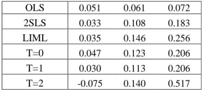
We now turn to the full model space and use the prior of Strachan and Inder (2004) for T = 2. We begin by presenting results which are not based on Bayesian model averaging. Table 5 gives frequentist and Bayesian estimates of the returns to schooling in the all-encompassing model (which includes all elements of X as exogenous regressors, all variables in Z as instruments, and treats all variables in y2 as endogenous). The point estimates of the
returns to schooling are similar using all approaches. The Bayesian posterior medians (for T = 0;1, 2) lie in between the 2SLS (11%) and the LIML estimates (15%). The 95% Bayesian credible intervals for T = 0;1are wider than 2SLS con…dence intervals but narrower than their LIML counterparts. However, the Bayesian credible interval with the priorT = 2is much wider. It includes even negative values, indicating that identi…cation might be poor11. The reason for the wider credible intervals with T = 2 is the non-existence of prior moments for .
In a BMA exercise it is typical to report not only averages over the whole model space, but also averages over restricted subspaces of the model space. For this purpose let us de…ne four binary indicators: Ie, Ir, Id and Ic which
equal one for a particular subset of the models (the value zero indicates all of the relevant models are included). The indicatorIe takes value one when all
variables in y2 are endogenous (i.e. no exogeneity restrictions are imposed).
Ir takes value 1 when the coe¢ cients of (ED76, AGE76) are both di¤erent
from 0.12 I
d takes value one when deu (the under-identi…cation discrepancy
measure) is above its own posterior median. Thus, Id takes value one when
identi…cation is stronger. Ic takes value one when NEARC4 (conventionally
considered to be a very important instrument) is included in the model as an instrument.
We begin with a discussion of returns to schooling estimates using BMA. These are given in Table 6. Results for BMA over the full model space are given in the rows labelled T = 0;1;2 in the column labelled Ie = 0. For
all of our three temperatures, our point estimate of returns to schooling is 0.015 and 95% credible intervals are fairly narrow. This point estimate is
11The Anderson canonical correlation LR test rejects the null of under-identi…cation
(p-value 0.0066) while the Sargan test fails to reject the validity of over-identifying restrictions (p-value 0.2159). However, the Stock-Yogo test fails to reject that 2SLS estimates might be subject to 30% or more bias due to weak identi…cation.
substantively lower than those in Table 5. For instance, with LIML we found a point estimate of 0.146, and 0.015 is outside the LIML 95% con…dence interval.
The other estimates in Table 6, using subsets of the model space, shed insight on why BMA is giving a lower estimate of returns to schooling than any of the other IV based approaches. Consider …rst what happens if we do BMA only over models in which all variables iny2 are endogenous (i.e. Ie=
1). It can be seen that results are much more consistent with the non-BMA results of Table 5. That is, the 95% credible interval for T = 0;1 exclude negative values and are centered at 10%. Just as we found in Table 5, the
T = 2 credible interval is now very wide (and even contains negative values). If we consider additional restrictions on the model space, the basic story (i.e. that only considering models where all variables iny2 are endogenous is
necessary to obtain results similar to those found using standard IV methods) is not altered. That is, conditioning on (Ir = 1; Id = 1) or (Ir = 1; Ic = 1)
does not change results in a substantive fashion.
Table 7 shows the prior and posterior percentiles of deu and this gives
evidence that identi…cation is much weaker when Ie = 1.13 This is a point
we will return to shortly.
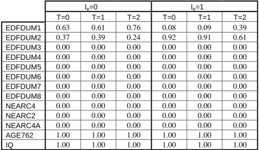
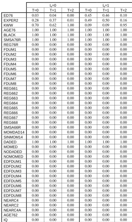
Tables 8, 9 and 10 show the probability that each variable enters each category. Tables 8 and 10 indicate that BMA has a strong preference for parsimony. Our full model space allows the elements of Z to enter as in-struments, as exogenous regressors or be excluded from the model. Tables 8 and 10 indicate that some are included as instruments, but most are excluded altogether from the model. Similarly, BMA allows the variables inX (which were always included in the models used to produce the results in Table 4) to be either exogenous regressors or be excluded from the model. Table 10 indicates most are excluded from the model. Table 9 provides us with strong evidence that two of the three elements of our “endogenous”y2 are actually
exogenous. And Figure 1, which shows BMA posterior densities (conditional on Ie = 1) of the correlations between v2 and u1, supports this view. Lastly,
the 2SLS estimate of the returns to schooling in the best model selected14 by
13The discrepancy measure de
o is not shown in some cases because there is probability one of just-identi…cation for each temperature, with the unused instruments not entering in the model at all. Two of these three instruments are AGE762 and IQ with probability 1. The third one could be either EDFDUM2 or EDFDUM1.
14By best model we mean the model that results from rounding the posterior probability
OLS 0.051 0.061 0.072 2SLS 0.033 0.108 0.183 LIML 0.035 0.146 0.256 T=0 0.047 0.123 0.206 T=1 0.030 0.113 0.206 T=2 -0.075 0.140 0.517
Table 5: Frequentist and Bayesian estimates and 95% confidence intervals of returns to schooling in the all encompassing model.
the RJMCMC is 0.012, with 95% con…dence interval being (0.004, 0.021). Putting all these …ndings together, we can now see why BMA is estimating returns to schooling as being lower than the traditional IV approaches of Table 5. Most importantly, the assumption that the elements of y2 truly
are endogenous is crucial to obtaining the traditional IV results. However, BMA is allocating relatively little weight to such models. Averaging over the full model space (i.e. including also models with exogeneity restrictions imposed) helps identi…cation and makes credible intervals of the returns to schooling narrower and centered on 1.5% for each of the 3 temperatures (Table 6). The posterior of deu con…rms that identi…cation is substantially
stronger if we use the full model space, anddeoshows that the over-identifying
restrictions hold (Table 7). The probability that only three elements of Z
enter as instruments is 100% forT = 0;1;2. The most likely instruments are AGE762 and IQ, followed by EFDUM1 and EFDUM2. A further di¤erence between BMA and non-BMA results arises since the former is much more parsimonious than the latter (and this holds for all of our priors).
In sum, this empirical example shows that our RJMCMC algorithm can be used to carry out BMA even in the very large model spaces that the re-searcher will often encounter in practice. It also shows that BMA can matter empirically. That is, BMA is leading to estimates of a feature of interest (returns to schooling) which di¤er in important ways from conventional es-timates. Furthermore, it provides insight into why such divergences occur and what aspects of model speci…cation have the most important impact on estimates of the returns to schooling.
Ie=0 Ie=1 T=0 0.004 0.015 0.088 0.015 0.099 0.120 T=0, Ir=1 0.043 0.085 0.127 0.087 0.105 0.123 T=0, Ir=1, Id=1 0.003 0.069 0.089 0.087 0.105 0.123 T=0, Ir=1, Ic=1 0.069 0.085 0.126 0.088 0.105 0.124 T=1 0.005 0.017 0.088 0.015 0.099 0.120 T=1, Ir=1 0.040 0.084 0.126 0.087 0.105 0.123 T=1, Ir=1, Id=1 0.004 0.068 0.088 0.087 0.105 0.123 T=1, Ir=1, Ic=1 0.067 0.084 0.125 0.088 0.105 0.124 T=2 0.005 0.014 0.024 -0.022 0.019 0.118 T=2, Ir=1 0.006 0.036 0.125 -0.291 0.104 0.523 T=2, Ir=1, Id=1 -0.002 0.025 0.048 -0.166 0.103 0.260 T=2, Ir=1, Ic=1 0.003 0.106 0.129 -0.998 0.108 1.338
Table 6: BMA posterior percentiles (2.5%, 50%, 97.5%) of returns to schooling. The columns underIe=1 correspond to the case in which
exogeneity restrictions are not considered, while those under Ie=0
refer to the case in which the model space includes also models with exogeneity restrictions.
Table 7: BMA posterior percentiles (2.5%, 50%, 97.5%) of (d~o,d~u). Ie=0 Ie=1 T=0 prior 1.11 299901 2460014 0.000 0.001 0.318 T=0 post 0.001 3.59 8.12 0.000 0.001 0.002 T=1 prior 1.35 270274 2367542 0.000 0.001 0.320 T=1 post 0.001 2.58 7.13 0.000 0.001 0.002 T=2 prior 0.047 435 3117025 0.000 0.002 0.542 u d~ T=2 post 0.001 0.401 7.35 0.000 0.001 0.002 T=0 prior 0.015 201 6223 T=0 post 0.000 0.000 0.005 T=1 prior 0.017 132 5897 T=1 post 0.000 0.000 0.005 T=2 prior 0.001 8.70 5482 o d~ T=2 post 0.000 0.000 0.004
Figure 1: Figure 1: Posterior density for the correlation between u and
v conditional on Ie = 1 and T = 1. From left to right the correlations
Ie=0 Ie=1 T=0 T=1 T=2 T=0 T=1 T=2 EDFDUM1 0.63 0.61 0.76 0.08 0.09 0.39 EDFDUM2 0.37 0.39 0.24 0.92 0.91 0.61 EDFDUM3 0.00 0.00 0.00 0.00 0.00 0.00 EDFDUM4 0.00 0.00 0.00 0.00 0.00 0.00 EDFDUM5 0.00 0.00 0.00 0.00 0.00 0.00 EDFDUM6 0.00 0.00 0.00 0.00 0.00 0.00 EDFDUM7 0.00 0.00 0.00 0.00 0.00 0.00 EDFDUM8 0.00 0.00 0.00 0.00 0.00 0.00 NEARC4 0.00 0.00 0.00 0.00 0.00 0.00 NEARC2 0.00 0.00 0.00 0.00 0.00 0.00 NEARC4A 0.00 0.00 0.00 0.00 0.00 0.00 AGE762 1.00 1.00 1.00 1.00 1.00 1.00 IQ 1.00 1.00 1.00 1.00 1.00 1.00
Table 8: Probability of variables inZ* entering in the model as an instrument (inz).
Ie = 0
T=0 T=1 T=2
ED76 0.05 0.04 0.05
EXPER2 0.07 0.06 0.47
KWW 0.98 0.98 1.00
Ie=0 Ie=1 T=0 T=1 T=2 T=0 T=1 T=2 ED76 0.03 0.04 0.00 0.45 0.46 0.10 EXPER2 0.28 0.37 0.01 0.49 0.50 0.16 KWW 0.70 0.62 1.00 0.09 0.09 0.95 AGE76 1.00 1.00 1.00 1.00 1.00 1.00 BLACK 1.00 1.00 1.00 1.00 1.00 1.00 SMSA76R 1.00 1.00 1.00 1.00 1.00 1.00 REG76R 0.00 0.00 0.00 0.00 0.00 0.00 FDUM1 0.00 0.00 0.00 0.00 0.00 0.00 FDUM2 0.00 0.00 0.00 0.00 0.00 0.00 FDUM3 0.00 0.00 0.00 0.00 0.00 0.00 FDUM4 0.00 0.00 0.00 0.00 0.00 0.00 FDUM5 0.00 0.00 0.00 0.00 0.00 0.00 FDUM6 0.00 0.00 0.00 0.00 0.00 0.00 FDUM7 0.00 0.00 0.00 0.00 0.00 0.00 FDUM8 0.00 0.00 0.00 0.00 0.00 0.00 REG661 0.00 0.00 0.00 0.00 0.00 0.00 REG662 0.00 0.00 0.00 0.00 0.00 0.00 REG663 0.00 0.00 0.00 0.00 0.00 0.00 REG664 0.00 0.00 0.00 0.00 0.00 0.00 REG665 0.00 0.00 0.00 0.00 0.00 0.00 REG666 0.00 0.00 0.00 0.00 0.00 0.00 REG667 0.00 0.00 0.00 0.00 0.00 0.00 REG668 0.00 0.00 0.00 0.00 0.00 0.00 SMSA66R 0.00 0.00 0.00 0.00 0.00 0.00 MOMDAD14 0.00 0.00 0.00 0.00 0.00 0.00 SINMOM14 0.00 0.00 0.00 0.00 0.00 0.00 DADED 1.00 1.00 1.00 1.00 1.00 1.00 MOMED 0.00 0.00 0.00 0.00 0.00 0.00 NODADED 0.00 0.00 0.00 0.00 0.00 0.00 NOMOMED 0.00 0.00 0.00 0.00 0.00 0.00 EDFDUM1 0.00 0.00 0.00 0.00 0.00 0.00 EDFDUM2 0.00 0.00 0.00 0.00 0.00 0.00 EDFDUM3 0.00 0.00 0.00 0.00 0.00 0.00 EDFDUM4 0.00 0.00 0.00 0.00 0.00 0.00 EDFDUM5 0.00 0.00 0.00 0.00 0.00 0.00 EDFDUM6 0.00 0.00 0.00 0.00 0.00 0.00 EDFDUM7 0.00 0.00 0.00 0.00 0.00 0.00 EDFDUM8 0.00 0.00 0.00 0.00 0.00 0.00 NEARC4 0.00 0.00 0.00 0.00 0.00 0.00 NEARC2 0.00 0.00 0.00 0.00 0.00 0.00 NEARC4A 0.00 0.00 0.00 0.00 0.00 0.00 AGE762 0.00 0.00 0.00 0.00 0.00 0.00 IQ 0.00 0.00 0.00 0.00 0.00 0.00
6
Conclusions
BMA has enjoyed an increasing popularity amongst econometricians work-ing with the regression model with a large number of exogenous regressors. The purpose of the present paper is to develop methods for BMA when endogeneity may be present. In such a case, any variable could be an en-dogenous variable, an exogenous variable or an instrument (and sometimes the researcher is unsure which category a variable belongs to). Doing BMA with such a setup is complicated by the huge model space that results and (in contrast to the case where all regressors are exogenous) the lack of avail-ability of analytical results for each model. To surmount these problems, this paper develops a RJMCMC algorithm which draws jointly from the model and parameter spaces. To surmount problems of slow convergence, we draw on ideas from the simulated tempering literature and introduce cold, hot and super-hot models into our algorithm. A further advantage of our algorithm is that draws of di¤erent temperatures can be used to carry out Bayesian inference under di¤erent priors. If we use the draws from the cold models we are doing BMA under an approximation to the posterior, if we use hot draws we are doing BMA using the prior of Drèze (1976) and if we use super-hot draws we are doing BMA using a prior such as that of Strachan and Inder (2004).
We illustrate our algorithm using the classic returns to schooling applica-tion of Card (1995). We …nd our RJMCMC algorithm to work e¢ ciently and empirical results show some interesting di¤erences between model averaging and conventional econometric methodologies.
References
Anderson, T. and Rubin, H., 1949, Estimation of the parameters of a sin-gle equation in a complete system of stochastic equations, Annals of Mathe-matical Statistics, 20, 46–63.
Anderson, T. and Rubin, H., 1950, The asymptotic properties of estima-tors of the parameters of a single equation in a complete system of stochastic equations, Annals of Mathematical Statistics, 21, 570-582.
Bauwens, L., Lubrano, M. and Richard, J.-F., 1999, Bayesian Inference
in Dynamic Econometric Models. Oxford: Oxford University Press.
Card, D., 1995, Using geographic variation in college proximity to esti-mate the return to schooling, inAspects of Labour Market Behaviour: Essays
in Honour of John Vandekamp edited by Louis N. Christo…des, E. Kenneth
Grant, and Robert Swidinsky. Toronto: University of Toronto Press.
Cohen-Cole, E., Durlauf, S., Fagan, J. and Nagin, D., 2009, Model un-certainty and the deterrent e¤ect of capital punishment, American Law and
Economics Review, forthcoming.
Drèze, J.H., 1976, Bayesian limited information analysis of the simulta-neous equations model, Econometrica, 44, 1045–1075.
Drèze, J.H. and Richard, J.F. 1983, Bayesian Analysis of Simultaneous Equations Systems. In Handbook of Econometrics, volume 1, edited by Z. Griliches and M.D. Intrilligator. Amsterdam: Elsevier Science.
Eicher, T.S., Lenkoski, A. and Raftery, A.E. (2009), Bayesian model av-eraging and endogeneity under model uncertainty: An application to devel-opment determinants, Working Paper no. 94, Center for Statistics and the Social Sciences, University of Washington.
Fernandez, C., Ley, E. and Steel, M., 2001, Benchmark priors for Bayesian model averaging, Journal of Econometrics, 100, 381-427.
Geyer, C. and Thompson, E., 1995, Annealing Markov Chain Monte Carlo with applications to ancestral inference, Journal of the American Statistical Association, 90, 909-920.
Green, P., 1995, Reversible jump Markov chain Monte Carlo computation and Bayesian model determination, Biometrika, 82, 711-732.
Greene, W., 2003, Econometric Analysis (Fifth edition), New Jersey: Prentice-Hall.
Hausman, J., 1983, Speci…cation and estimation of simultaneous equa-tions models, in Z. Griliches and M. Intriligator, eds., Handbook of
Holmes, C., Denison, D. and Mallick, B., 2002, Bayesian model order determination and basis selection for seemingly unrelated regression,Journal of Computational and Graphical Statistics, 11, 533–551.
Johansen, S., 1988, Statistical Analysis of Cointegration Vectors,Journal
of Economic Dynamics and Control, 12, 231-254.
Johansen, S., 1995,Likelihood-Based Inference in Cointegrated Vector
Au-toregressive Models. Oxford: Oxford University Press.
Kleibergen, F. and Paap, R., 2002, Priors, posteriors and bayes factors for a Bayesian analysis of cointegration, Journal of Econometrics, 111, 223-249. Kleibergen, F. and van Dijk, H., 1998, Bayesian simultaneous equations analysis using reduced rank structures, Econometric Theory, 14, 699-744.
Koop, G., 2003,Bayesian Econometrics. Chichester: Wiley.
Koop, G., Leon-Gonzalez, R. and R. Strachan, 2010, E¢ cient posterior simulation for cointegrated models with priors on the cointegration space,
Econometric Reviews, 29, 224-242.
Liu, J.S., 2001, Monte Carlo Strategies in Scienti…c Computing. Berlin: Springer.
Madigan, D. and York, J., 1995, Bayesian graphical models for discrete data, International Statistical Review, 63, 215-232.
Madan, D.B. and Seneta, E., 1990, The Variance-Gamma (V.G) Model for Share Market Returns, Journal of Business 63, 511-524.
Marinari, E. and Parisi, G., 1992, Simulated tempering: a new Monte Carlo scheme., Europhysics Letters, 19, 451-458.
Muirhead, R.J., 1982, Aspects of Multivariate Statistical Theory. New York: Wiley.
Sargan, J., 1958, The estimation of economic relationships using instru-mental variables, Econometrica, 26, 393-415.
Strachan, R. and Inder, B., 2004, Bayesian analysis of the error correction model, Journal of Econometrics, 123, 307-325.
Waagepetersen, R. and Sorensen, D., 2001, A tutorial on reversible jump MCMC with a view toward applications in QLT mapping,International Sta-tistical Review, 69, 49-61.
Zellner, A., 1971,An Introduction to Bayesian Inference in Econometrics. New York: John Wiley and Sons.
Zellner, A., Bauwens, L. and van Dijk, H.K., 1988, Bayesian speci…cation analysis and estimation of simultaneous equation models using Monte Carlo methods, Journal of Econometrics, 38, 39-72.
Data Appendix
The data used in this paper was used in Card (1995) and provided on Card’s website: http://emlab.berkeley.edu/users/card/data_sets.html. These sources provide complete information about this data set. We useN = 2040
observations on individuals from 1976 from the National Longitudinal Survey (this is the original cohort). In our modelling approach, each variable must either be the main dependent variable of interest (y1), another endogenous
variable (y2), a potential regressor (X ) or a variable which could either be
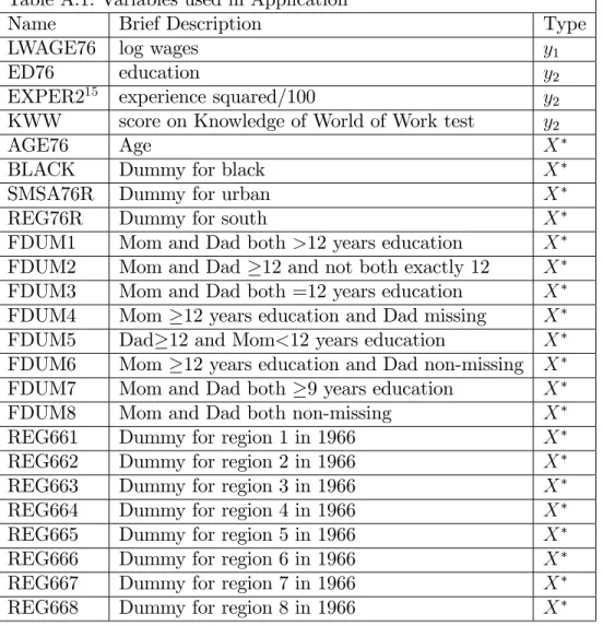
an instrument or a regressor (Z ). We follow Card (1995) in our classi…cation of variables and refer the reader to his paper for a justi…cation. The following is a summary of the 45 variables we use along with the category each belongs in. All variables refer to 1976 unless otherwise noted.
Table A.1: Variables used in Application
Name Brief Description Type
LWAGE76 log wages y1
ED76 education y2
EXPER215 experience squared/100 y
2
KWW score on Knowledge of World of Work test y2
AGE76 Age X
BLACK Dummy for black X
SMSA76R Dummy for urban X
REG76R Dummy for south X
FDUM1 Mom and Dad both>12 years education X
FDUM2 Mom and Dad 12 and not both exactly 12 X
FDUM3 Mom and Dad both =12 years education X
FDUM4 Mom 12 years education and Dad missing X
FDUM5 Dad 12 and Mom<12 years education X
FDUM6 Mom 12 years education and Dad non-missing X
FDUM7 Mom and Dad both 9 years education X
FDUM8 Mom and Dad both non-missing X
REG661 Dummy for region 1 in 1966 X
REG662 Dummy for region 2 in 1966 X
REG663 Dummy for region 3 in 1966 X
REG664 Dummy for region 4 in 1966 X
REG665 Dummy for region 5 in 1966 X
REG666 Dummy for region 6 in 1966 X
REG667 Dummy for region 7 in 1966 X
REG668 Dummy for region 8 in 1966 X
15Card de…nes experience as age - education - 6 and includes it, together with EXPER2,
as an endogenous explanatory variable while age is included as an instrument. To avoid having a singular covariance matrix, we instead include age as a regressor (i.e. in X ) and exclude experience from the analysis (but still include EXPER2 in y2). Note that
our speci…cation is just a reparameterization of that of Card (1995), and in our case the return to schooling is given by the sum of the coe¢ cients of ED76 and AGE76.
Table A.1 (continued): Variables used in Application
Name Brief Description Type
SMSA66R Dummy for urban in 1966 X
MOMDAD14 Dummy for living with mom and dad at 14 X
SINMOM14 Dummy for living with single mom at 14 X
DADED Dad’s years of schooling X
MOMED Mom’s years of schooling X
NODADED Dummy for DADED imputed X
NOMOMED Dummy for MOMED imputed X
EDFDUM1 FDUM1*NEARC4 Z EDFDUM2 FDUM2*NEARC4 Z EDFDUM3 FDUM3*NEARC4 Z EDFDUM4 FDUM4*NEARC4 Z EDFDUM5 FDUM5*NEARC4 Z EDFDUM6 FDUM6*NEARC4 Z EDFDUM7 FDUM7*NEARC4 Z EDFDUM8 FDUM8*NEARC4 Z
NEARC4 Dummy grew up near any 4 year college Z
NEARC2 Dummy grew up near 2 year college Z
NEARC4A Dummy grew up near 4 year public college Z
AGE762 Age squared Z
Technical Appendix
Algorithm
To illustrate the general principle underlying the algorithm we use, suppose
that the vector of unknown parameters in model M can be decomposed
as M = ( 1M; 2M). Let q(M( )jM(r)) be a proposal density for models.
Because we are going to de…ne a move conditional on 1M, we require that
q(M( )jM(r))gives zero probability to modelsM( ) in which the dimension of
1M changes. Let q( 2Mj 1M; M) be a proposal density for 2M. The general
expression for the acceptance probability for a move from ( (r)
2M(r); M
(r)) to
( ( )2M( ); M
( ))conditional on
1M can be found for example at Waagepetersen
and Sorensen (2001) and it is equal to:
a= min ( 1;q(M (r) jM( )) q(M( )jM(r)) p(Y; 1M; ( ) 2M( )jM ( )) p(Y; 1M; (r) 2M(r)jM(r)) q( (2rM)(r)j 1M; M (r)) q( ( )2M( )j 1M; M( )) p(M( )) p(M(r)) )
where p(M ) is the prior probability of model M . Following the strategy of Holmes and Held (2006), we always choose q( ( )2M( )j 1M; M
( )) to be the
optimal choice p( ( )2M( )jY; 1M; M
( )), that is, the conditional posterior of 2M given 1M and M = M( ). As a consequence of choosing such proposal
density, the expression for a simpli…es to:
a= min 1;q(M (r) jM( )) q(M( )jM(r)) p(Y; 1MjM( )) p(Y; 1MjM(r)) p(M( )) p(M(n)) (7) where p(Y; 1MjM) = Z p(Y; 1M; 2MjM)d 2M = Z p( 1M; 2MjM)p(Yj 1M; 2M; M)d 2M
We use two indexes to describe the model space: (M; T), where T takes values0(for cold models, which are based on an approximation to the poste-rior),1(for hot models, which use Drèze’s prior) and 2 (for super-hot models, which use another prior p ( ; jM), where = ( 0; 0; vec( 2x); vec( 2z)0).
Let the prior probability of each(M; T)be denoted asp(M; T) = p(T)p(MjT). The functionp(T)can be chosen as a tuning parameter to ensure that the al-gorithm spends enough time at each temperature. Let ( (r); (r); M(r); T(r))
be the value of ( ; ; M; T) in the rth draw from the algorithm. Our
pro-posal density for(M; T), which we denote as q(M( ); T( )jM(r); T(r)), is such that with probability T(r) a candidate value for temperature (T( )) is drawn
from some distribution (q(T( )
jT(r))) while the model restrictions remain
constant (i.e. M( ) = M(r)) and with probability (1 T(r)) a candidate
model (M( ))is drawn from some distribution (q(M( )
jM(r); T(r)))while the
value of temperature remains constant (T( ) = T(r)). The values de…ning
T(r) are denoted as 1 and 2, with 1 2. These are constants that,
together with p(T), can be calibrated in the burn-in period to ensure that the algorithm visits each temperature enough times16.
The(r+1)thvalue of( ; ; M; T)(denoted as( (r+1); (r+1); M(r+1); T(r+1))
is obtained as follows: IfT(r) = 0:
Draw u from a uniform in(0;1).
If u < 1:(propose a change from a cold model to the analogous hot one conditioning only on 2z).
–Fix M(r+1) = M(r). Fix T(r+1) = 1 with probability a and …x
T(r+1)= 0 with probability(1 a), wherea is de…ned as:
a= min ( p(M(r+1); T(r+1) = 1)p(Y; (r) 2zjM(r+1); T(r+1) = 1) p(M(r+1); T(r+1) = 0)p(Y; (r) 2zjM(r+1); T(r+1) = 0) ;1 ) –If T(r+1) = 1 draw (r+1) conditional on ( (r) 2z; M(r+1); T(r+1))
and then draw( (2rz+1); (r+1); (r+1); (r+1)
2x )conditional on( (r+1)
; M(r+1); T(r+1)).
–IfT(r+1) = 0draw( (r+1); (r+1))conditional on(M(r+1); T(r+1)).
Ifu 1: (propose a change from a cold model to another cold model, changing any of the model restrictions)
–Fix T(r+1) = T(r) = 0. Draw a candidate value M( ) from a
pro-posal distributionq(MjM(r); T(r+1) = 0). This proposal distribu-tion changes any of the model restricdistribu-tions with some probability.
16Liu (2001, p. 210) recommends that simulated tempering algorithms are tuned so that
FixM(r+1) =M( ) with probabilityaand …xM(r+1) =M(r) with
probability (1 a), where a is de…ned as:
a= min p(M ( ); T(r+1))p(Y jM( ); T(r+1))q(M(r) jM( ); T(r+1)) p(M(r); T(r+1))p(YjM(r); T(r+1))q(M( )jM(r); T(r+1));1 –Draw ( (r+1); (r+1)) conditional on (M(r+1); T(r+1)). IfT(r) = 1:
Draw u from a uniform in(0;1).
If u < 1: (propose a change from a hot model to the analogous cold one conditioning only on 2z).
–Fix M(r+1) = M(r). Fix T(r+1) = 1 with probability a and …x
T(r+1)= 0 with probability(1 a), wherea is de…ned as:
a= min ( p(M(r+1); T(r+1) = 0)p(Y; (r) 2zjM(r+1); T(r+1) = 0) p(M(r+1); T(r+1) = 1)p(Y; (r) 2zjM(r+1); T(r+1) = 1) ;1 ) –If T(r+1) = 1 draw (r+1) conditional on ( (r) 2z; M(r+1); T(r+1))
and then draw( (2rz+1); (r+1); (r+1); (r+1)
2x )conditional on( (r+1)
; M(r+1); T(r+1)).
–IfT(r+1) = 0draw( (r+1); (r+1))conditional on(M(r+1); T(r+1)).
If 1 u 2: (propose a change from a hot model to another hot
model conditioning on ).
–Fix T(r+1) = T(r) = 1. Draw a candidate value M( ) from a
pro-posal distribution q(MjM(r); T(r+1)). This distribution proposes models that could change any restriction except for those related to . FixM(r+1) =M( )with probabilityaand …xM(r+1) =M(r)
with probability (1 a), where a is de…ned as:
a= min p(M
( ); T(r+1))p(Y; (r)
jM( ); T(r+1))q(M(r)
jM( ); T(r+1))