Tonolini, F., Jensen, B. S. and Murray-Smith, R. (2019) Variational Sparse
Coding. In: Conference on Uncertainty in Artificial Intelligence (UAI
2019), Tel Aviv, Israel, 22-25 July 2019
There may be differences between this version and the published version.
You are advised to consult the publisher’s version if you wish to cite from
it.
http://eprints.gla.ac.uk/191553/
Deposited on 31 July 2019
Enlighten – Research publications by members of the University of
Glasgow
Variational Sparse Coding
Francesco Tonolini
School of Computing Science University of Glasgow
Glasgow, UK
Bjørn Sand Jensen
School of Computing Science University of Glasgow
Glasgow, UK
Roderick Murray-Smith
School of Computing Science University of Glasgow
Glasgow, UK
Abstract
Unsupervised discovery of interpretable fea-tures and controllable generation with high-dimensional data are currently major chal-lenges in machine learning, with applications in data visualisation, clustering and artificial data synthesis. We propose a model based on variational auto-encoders (VAEs) in which interpretation is induced through latent space sparsity with a mixture of Spike and Slab dis-tributions as prior. We derive an evidence lower bound for this model and propose a spe-cific training method for recovering disentan-gled features as sparse elements in latent vec-tors. In our experiments, we demonstrate supe-rior disentanglement performance to standard VAE approaches when an estimate of the num-ber of true sources of variation is not available and objects display different combinations of attributes. Furthermore, the new model pro-vides unique capabilities, such as recovering feature exploitation, synthesising samples that share attributes with a given input object and controlling both discrete and continuous fea-tures upon generation.
1
INTRODUCTION
Variational auto-encoders (VAEs) offer an efficient way of performing approximate posterior inference with oth-erwise intractable generative models and yield proba-bilistic encoding functions that can map complicated high-dimensional data to lower dimensional representa-tions (Kingma & Welling, 2013; Rezende et al., 2014; Sønderby et al., 2016). Making such representations meaningful, however, is a particularly difficult task and currently a major challenge in representation learning
(Burgess et al., 2018; Tomczak & Welling, 2018; Kim & Mnih, 2018). Large latent spaces often give rise to many latent dimensions that do not carry any information, and obtaining codes that properly capture the complexity of the observed data is generally problematic (Tomczak & Welling, 2018; Higgins et al., 2017b; Burgess et al., 2018).
In the case of linear mappings, sparse coding offers an el-egant solution to the aforementioned problem; the repre-sentation space is induced to be sparse. In such a way, the encoding function can exploit a high-dimensional space to model a large number of possible features, while being encouraged to use a small subset of non-zero elements to describe each individual observation (Olshausen & Field, 1996a;b). Due to their efficiency of representa-tion, sparse codes have been used in many learning and recognition systems, as they provide easier interpretation when processing natural data (Lee et al., 2007; Bengio et al., 2013). Biological system have also notably been proven to exploit signal sparsity for visual perception (Olshausen & Field, 1996a;b).
In this work, we aim to extend the aforementioned ca-pability of linear sparse coding to non-linear probabilis-tic generative models thus allowing efficient, informative and interpretable representations in the general case. To this end we formulate a new variation of VAEs in which we employ a sparsity inducing prior and a discrete mix-ture recognition model based on the Spike and Slab dis-tribution. We construct a flexible sparse prior as a com-bination of Spike and Slab recognition models through auxiliary pseudo-inputs. We derive a non-trivial analyti-cal evidence lower bound (ELBO) for the model and de-sign a pre-training procedure that avoids mode collapse.1
In our experiments, we study feature disentanglement in the general situation where no estimate of the number of
1
An implementation of the VSC model is
avail-able from https://github.com/ftonolini45/
ground truth features is available and different features can be present or absent in each observed data exam-ple. We show how our model considerably outperforms traditional disentanglement approaches (Higgins et al., 2017a; Gao et al., 2019) in such conditions. We then consider two benchmark data sets, Fashion-MNIST and UCI HAR, and demonstrate how the variational sparse coding (VSC) model recovers sparse representations that properly capture the mixed discrete and continuous na-ture of their variability. We further show how such repre-sentations can be used to investigate feature relationships among different objects and classes and perform condi-tional generation completely unsupervisedly.
2
BACKGROUND
2.1 SPARSE CODING
Sparse coding aims to approximately represent observed signals with a weighted linear combination of few un-known basis vectors (Lee et al., 2007; Bengio et al., 2013). The task of determining the optimal basis is gen-erally formulated as an optimisation problem, where a reconstruction cost and a sparsity cost of the embedded representations are jointly minimised with respect to the coefficients of a linear transformation. Sparse coding makes the important realisation that, though large en-sembles of natural signals need many variables to be de-scribed, individual samples can be well represented by a small subset of such variables. This realisation is sup-ported by substantial empirical evidence and pioneering work by Olshausen & Field (1996a) also showed that the visual cortex in mammals processes information as sparse signals, demonstrating that biological learning ex-ploits sparsity in natural images similarly to sparse cod-ing based models. Olshausen & Field (2004) provide a comprehensive review of linear sparse coding.
Sparse coding can be probabilistically interpreted as a generative model, where the observed signals are gen-erated from unobserved latent variables through a linear process (Lee et al., 2007; Bengio et al., 2013). The model can then be described with a latent prior distribution, which assigns high density to sparse latent variables, and a likelihood distribution, which quantifies the reconstruc-tion density given a latent embedding. In fact, perform-ing maximum a posteriori (MAP) estimation with such models recovers the common formulation of sparse cod-ing described above. Previous work has also demon-strated variational inference with sparse coding proba-bilistic models, exploiting algorithms based on EM infer-ence (Titsias & L´azaro-Gredilla, 2011; Goodfellow et al., 2012). However, EM inference becomes intractable for more complicated non-linear posteriors and a large
num-ber of input vectors (Kingma & Welling, 2013), making such an approach unsuitable to scale to our target mod-els.
Conversely, some work has been done in generalising sparse coding to non-linear transformations, by defin-ing sparsity on Riemannian manifolds (Ho et al., 2013; Cherian & Sra, 2017). These generalisations, however, are not probabilistic, as they define a non-linear equiv-alent of MAP inference and are limited to simple mani-folds due to the need to compute the manifold’s logarith-mic map.
2.2 VARIATIONAL AUTO-ENCODERS
Variational auto-encoders (VAEs) are models for un-supervised efficient coding that aim to maximise the marginal likelihood p(x) = Q
p(xi) with respect to
some decoding parameters θ of the likelihood func-tion pθ(x|z) and encoding parameters φ of a
recogni-tion modelqφ(z|x)(Kingma & Welling (2013); Rezende
et al. (2014); Pu et al. (2016)).
The VAE model is defined as follows; an observed vec-torxi ∈ RM×1 is assumed to be drawn from a
likeli-hood functionpθ(x|z). Common choices are a Gaussian
or a Bernoulli distribution. The parameters ofpθ(x|z)
are the output of a neural network having as input a la-tent variablezi ∈RJ×1. The latent variable is assumed
to be drawn from a prior p(z) which can take differ-ent parametric forms. In the most common VAE im-plementations, the prior takes the form of a multivariate Gaussian with identity covarianceN(z; 0, I) (Kingma & Welling, 2013; Rezende et al., 2014; Higgins et al., 2017b; Burgess et al., 2018; Yeung et al., 2017). The aim is then to maximise a joint posterior distribution of the form p(x) = Q
i R
pθ(xi|z)p(z)dz, which for an
arbitrarily complicated conditionalp(x|z)is intractable. To address this intractability, VAEs introduce a recogni-tion modelqφ(z|x)and define an evidence lower bound
(ELBO) to be estimated in place of the true posterior, which can be formulated as
logpθ(xi) = log Z pθ(xi|z)p(z) qφ(z|xi) qφ(z|xi) dz≥ −DKL(qφ(z|xi)||p(z)) +Eqφ(z|xi)[logpθ(xi|z)]. (1)
The ELBO is composed of two terms; a prior term, which encourages minimisation of the KL divergence between the encoding distributions and the prior, and a recon-struction term, which maximises reconrecon-struction likeli-hood. The ELBO is then maximised with respect to the model’s parametersθandφ.
2.2.1 Interpretation in VAEs
Obtaining informative and interpretable representations of unlabelled data is currently a major objective of un-supervised learning. VAEs have been recently consid-ered as ideal models to obtain such representations, as they rely on a low dimensional latent space that nec-essarily embeds information about the observation they model. Inducing interpretation in a VAE latent space is generally formulated as a feature disentanglement prob-lem; assuming observed data is generated from hidden interpretable factors of variation, the task is to obtain a latent space in which such factors are aligned with the axis. The commonly adopted method to enhance the dis-entanglement of features in a VAE is to assign a larger weight to the KL divergence component in equation 1. Models following this approach are known asβ-VAEs, and they allow controllable improvement of latent disen-tanglement, at the expense of reconstruction likelihood (Higgins et al., 2017a; Burgess et al., 2018). Several al-ternative methods to improve disentanglement have been proposed. Recent works extended theβ-VAE to explic-itly control total correlation between latent dimensions, expressing it as a penalty term that quantifies disentan-glement (Chen et al., 2018; Gao et al., 2019). Kim & Mnih (2018) proposed an algorithm to directly induce factorisation, demonstrating a more favourable trade-off between disentanglement and reconstruction accuracy. These approaches have proven promising, however they rely on the assumption that target features are always present in every observation with continuously varying values. Differently from these, the model presented here relies on the sparse coding realisation of natural signals, assuming that individual observations are described by only a small subset of a large ensemble of possible fea-tures. Furthermore, we assume no knowledge of the number of source factors.
2.2.2 Discrete Latent Variables and Sparsity in VAEs
Discrete latent distributions are a closely related theme to sparsity, as exactly sparse PDFs involve sampling from some discrete variables. Nalisnick & Smyth (2017) and Singh et al. (2017) model VAEs with a Stick-Breaking Process and an Indian Buffet Process priors respectively in order to allow for stochastic dimensionality in the la-tent space. In such a way, the prior can set unused di-mensions to zero. However, the resulting representations are not truly sparse; the same elements are set to zero for every encoded observation. The scope of these works is dimensionality selection rather than sparsification. Other models which present discrete variables in their la-tent space have been proposed in order to capture discrete
features in natural observations. Rolfe (2017) models a discrete latent space composed of continuous variables conditioned on discrete ones in order to capture both dis-crete and continuous sources of variation in observations. Similarly motivated, van den Oord et al. (2017) per-form variational inference with a learned discrete prior and recognition model. The resulting latent spaces can present sparsity, depending on the choice of prior. How-ever, they do not induce directly sparse statistics in the latent space.
Other works model sparsity more directly. Yeung et al. (2017) propose to learn a deterministic selection vari-able that dictates which latent dimensions the recogni-tion model should exploit in the latent space. In such a way, different embeddings can exploit different com-binations of variables, which achieves the goal of coun-teracting over-pruning. This approach does result into sparse latent variables. However, only the continuous components are treated variationally, while the activa-tion of elements is deterministic. More recently, Mathieu et al. (2019) modelled sparsity in the latent space with a mixture of Gaussians models using a narrow Gaussian component to encourage elements to be close to zero. In their work, a continuous relaxation of sparsity is mod-elled in the latent space, as elements are not encouraged to be zero exactly, but only close to zero by the narrow Gaussian component of the prior.
Differently from these prior works, we directly model the mixed continuous-discrete nature of sparsity in the latent space through an exactly sparse prior and find a suitable evidence lower bound and training procedure to perform approximate variational inference.
3
VARIATIONAL SPARSE CODING
We propose to use the framework of VAEs to perform approximate variational inference with neural network sparse coding architectures. With this approach, we aim to discover and discern the non-linear features that con-stitute variability in data and represent them as few non-zero elements in sparse vectors.
3.1 RECOGNITION MODEL
In order to encode observations as sparse vectors in the latent space, the recognition model is chosen to be a Spike and Slab distribution. The Spike and Slab dis-tribution is defined over two variables; a binary spike variablesj and a continuous slab variablezj (Mitchell
& Beauchamp, 1988). The spike variable is either one or zero with defined probabilitiesγand(1−γ) respec-tively and the slab variable has a distribution which is either a Gaussian or a Delta function centered at zero,
conditioned on whether the spike variable is one or zero respectively. The resulting recognition model is
qφ(z|xi) = J Y
j=1
[γi,jN(zi,j;µz,i,j, σ2z,i,j)
+(1−γi,j)δ(zi,j)],
(2)
where the distribution parameters µz,i,j, σz,i,j2 andγi,j
are the outputs of a neural network having parametersφ and inputxi,J is the number of latent dimensions and
δ(·)indicates the Dirac delta function centered at zero. A description of the recognition model neural network can be found in supplementary A.2.
3.2 PRIOR DISTRIBUTION
In order to induce sparsity in the latent space while al-lowing the model to flexibly adjust to represent differ-ent combinations of features, we build upon two re-cent advances in VAEs. Following the prior structure presented in Tomczak & Welling (2018), we build the prior with recognition models qφ(z|xu) from
pseudo-inputsxu, which are trained along with the networks’
weights. However, differently from this previous work, which builds the prior with the sum of all pseudo inputs’ encodingsp(z) = U1P
uqφ(z|xu), we implement a
clas-sifieru∗=Cω(xi)with parametersωto select a specific
pseudo-input xu∗ and consequentially a single compo-nent qφ(z|xu∗) for an observation xi, hence assuming that each observationxiis generated from a single
com-ponent in the latent space. This feature is similar to the latent variable selection presented in Yeung et al. (2017), with the difference that the selector in the VSC model as-signs a different prior for each observations, rather then different latent dimensions. The sparse prior is then
ps(z) =qφ(z|xu∗), u∗=Cω(xi),
(3)
whereCω(x)is a neural network classifier. The use of
the classifierCω(x)rather than taking the whole
ensem-ble as prior allows us to compute the KL divergence an-alytically, hence rendering optimisation efficient while maintaining the flexibility of a prior composed of mul-tiple PDFs. A detailed description of the selection func-tionCω(x)can be found in supplementary A.3.
3.3 VSC OBJECTIVE FUNCTION
As in the standard VAE setting, we aim to perform ap-proximate variational inference by maximising an ELBO of the form detailed in equation 1, with the Spike and Slab probability density function of equation 3 as prior and the recognition model of equation 2. Additionally,
we need to infer a defined prior sparsityαin the latent space. This is done by inducing the average Spike prob-ability of each pseudo-input’s recognition model γu to match the prior oneα. a sparsity KL divergence penalty termDKL(γu||α)is then minimised jointly to the
max-imisation of the ELBO
arg max θ,φ,ω,xu X i −DKL(qφ(z|xi)||qφ(z|xu∗)) +Eqφ(z|xi)[logpθ(xi|z)]−J·DKL(γu∗||α). (4)
The KL divergence between the pseudo-input’s prior and target sparsityDKL(γu∗||α)has a simple form and can
readily be differentiated with respect to the weights and pseudo-inputs. This term induces the encodings to have the prior sparsity on average, acting similarly to the ag-gregate posterior regularisation term described in Math-ieu et al. (2019). In the following subsections, we elabo-rate on the remaining two terms: the reconstruction and KL divergence terms of the ELBO.
3.3.1 Reconstruction Term
The reconstruction component of the ELBO is estimated stochastically as follows Eqφ(z|xi)[logpθ(xi|z)]' 1 L L X l=1 logpθ(xi|zi,l), (5)
where the sampleszi,l are drawn from the recognition
modelqφ(z|xi)andLis the number of such draws. As
in the standard VAE, to make the reconstruction term dif-ferentiable with respect to the encoding parametersφ, we employ a reparameterization trick to draw fromqφ(z|xi).
To parametrise samples from the discrete binary compo-nent ofqφ(z|xi) we use a continuous relaxation of
bi-nary variables analogous to that presented in Maddison et al. (2017) and Rolfe (2017). We make use of two aux-iliary noise variables andη, normally and uniformly distributed respectively. is used to draw from the Slab distributions, resulting in a reparametrisation analo-gous to the standard VAE (Kingma & Welling, 2013). η is used to parametrise draws of the Spike variables through a non-linear binary selection functionT(yi,l).
The two variables are then multiplied together to obtain the parametrised draw fromqφ(z|xi). A more detailed
description of the reparametrisation of sparse samples is reported in supplementary B.
3.3.2 Spike and Slab KL Divergence
KL divergences with discrete mixture PDFs have been used in various discrete latent variables models (Rolfe, 2017; Nalisnick & Smyth, 2017). However, in these works, they are estimated and optimised stochastically.
Gal (2016) derives an analytic form for a particular case in which the recognition model contains the prior. Dif-ferently form these, we derive a closed-form expression for the KL divergence between two arbitrary Spike and Slab distributions, hence rendering the optimisation of the ELBO for our model of comparable complexity to the standard VAE case.
By solving the KL divergence between the prior of equa-tion 3 and the recogniequa-tion model of equaequa-tion 2 we derive with a novel approach the closed-form expression DKL(qφ(z|xi)||qφ(z|xu∗)) = = J X j γi,j logσz,u∗,j σz,i,j + σz,i,j+ (µz,i,j−µz,u∗,j)2
2σz,u∗,j −1 2 + (1−γi,j) log 1−γi,j 1−γu∗,j +γi,jlog γi,j γu∗,j . (6)
A detailed derivation of this expression is reported in supplementary C. This expression naturally presents two components. The first term in the sum is the negative KL divergence between the distributions of the Slab vari-ables, multiplied by the probability ofzi,jbeing non-zero
γi,j. This component gives a similar regularisation to
that of the standard VAE and encourages the Gaussian components of the recognition model to match those of the prior, proportionally to the Spike probabilitiesγi,j.
The second term is the negative KL divergence between the distributions of the Spike variables, which encour-ages the probabilities of the latent variables being non-zeroγi,jto match those of the pseudo-input priorγu∗,j.
3.4 TRAINING
The VSC model is trained by maximizing the objective function in equation 4 using gradient descent, with the KL divergence of equation 6 and the empirical recon-struction term of equation 5. As other VAE models, VSC suffers from the inherent problem of posterior collapse; during training, certain latent variables tend to store all information about the encoded observations while the re-maining ones perfectly satisfy the KL divergence con-straint. In a VSC model with a very low prior Spike prob-abilityαthis results in a dimensionality collapse; some latent variables are set to zero for almost all encodings, while others store most of the information necessary to represent data. This may be desirable in some settings, such as dimensionality selection, but hinders the ability to adequately describe observations with different com-binations of recovered features.
To counteract the aforementioned posterior collapse
Algorithm 1Training the VSC Model
Inputs: observations x; initial model parameters,
{θ(0), φ(0), ω(0),x(0)
u }; user-defined latent
dimensional-ity,J; user-defined prior sparsity level,α; user-defined number of warm-up steps,Nwarmup; user-defined linear
increment in warm-up coefficient λ, ∆λ; user-defined number of iterations,Niter; user-defined number of
sam-ples,L, used in estimating the reconstruction term.
1: λ(k=0)←0
2: forthek’thiterationin[0 :Niter−1]
3: forthei’thobservation
4: zi,l∼qφ(k),λ(k)(z|xi) ∀l∈[1 :L] (Eq.5)
5: E(ik)←P
llogpθ(k)(xi|zi,l) (Eq.5)
6: u∗←Cω(k)(xi) (Eq.3) 7: K(ik)←DKL(qφ(k)(z|xi)||qφ(k)(z|xu∗)) 8: D(ik)←J·DKL(γu∗||α) (Eq.6) 9: end 10: F(k)=P i E(ik)−Ki(k)−D(ik) (Eq.4) 11: θ(k+1), φ(k+1), ω(k+1),x(k+1) u ←arg max(F(k)) (Eq.4)
12: ifλ(k)<1andk > Nwarmup (Eq.7)
13: λ(k+1)←λ(k)+ ∆λ
14: else
15: λ(k+1)←λ(k)
16: end 17: end
effect, we employ a straightforward Spike variable warm-up strategy. During a pre-training phase, the recognition modelqφ(z|xi)is modified as follows:
qφ,λ(z|xi) = J Y
j=1
[γi,jN(zi,j;λµz,i,j, λσz,i,j2
+ (1−λ)) + (1−γi,j)δ(zi,j)],
(7)
whereλis a constant which is initially set to zero, then linearly increased from zero to one and lastly set equal to one throughout training. Whenλis equal to zero, the Slab components of the latent variables is fixed to a zero mean and unit covariance Gaussian. This implies that the recognition model can initially store information only in the Spike variables patterns, similarly to a binary encod-ing, hence forcing latent vectors from different observa-tions to activate different elements. Asλis increased to one, the model can store more information in the contin-uous Slab variables, however maintaining different com-binations of active latent variables for distinct observa-tions.
In summary, we contribute two main elements of nov-elty; the derivation of a closed form expression for the Spike and Slab KL divergence and the Spike warm-up strategy to avoid posterior collapse. Both are crucial in handling the mixed continuous-discrete nature of sparse representations and efficiently train the proposed model, hence obtaining sparse probabilistic representation of ob-servations. For completeness we outline the training pro-cedure in Algorithm 1. The values for each user defined parameters we employ in our experiments are reported in supplementary D. The maximisation at each iteration is carried out as an ADAM optimisation step.
4
EXPERIMENTS
4.1 ELBO EVALUATION
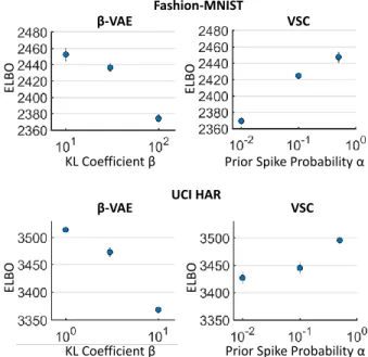
We evaluate and compare the ELBO values for VSC and β-VAE models. β-VAEs are VAEs in which the KL divergence term of equation 1 is assigned a control-lable weight β. Typically, they are used with a coef-ficient β greater than one to induce interpretation Hig-gins et al. (2017a). We make use of the Fashion-MNIST dataset, composed of28×28grey-scale images of dif-ferent pieces of clothing (Xiao et al., 2017), and the UCI HAR dataset, which consists of filtered accelerometer signals from mobile phones worn by different people during common activities (Anguita et al., 2012). In all cases, the latent space is chosen to have60latent dimen-sions and the neural networks of the two models are of equal capacity. For theβ-VAE we vary theβcoefficient, while for the VSC model we vary the prior spike proba-bilityα. Further details can be found in supplementary D.1. Results are shown in figure 1.
Overall, the ELBO values for the VSC model are com-parable to those recovered withβ-VAEs and a standard VAE (β = 1). The VSC results in lower ELBO values at decreasing prior spike probabilityα, similarly to the trend experienced by theβ-VAE at increasing KL coef-ficientβ. In fact, the two models present a similar be-haviour; as more structure is imposed in the latent space by enforcing a ‘stronger’ prior, the ELBO is necessarily reduced. The VSC model, however, imposes structure in the latent space through sparsity, rather than an increased weight on the KL divergence term of the ELBO. In the next subsection we show how this subtle difference re-sults into important representation advantages.
4.2 FEATURE DISENTANGLEMENT
We investigate the VSC model’s ability to disentangle generating features and align them with the latent space axis. To do so, we make use of an artificial dataset, where
the different examples are synthesised from a set of pa-rameters and therefore the generative source features are known and can be used as ground truth. Previous work similarly evaluated disentanglement with artificial sam-ples (Higgins et al., 2017a; Kim & Mnih, 2018). Data sets used in these investigations, however, contain signals generated by altering each feature continuously, leading to all examples expressing variability in all the generat-ing factors. Followgenerat-ing a sparse realisation of natural sig-nals, we are instead interested in situations where groups of generating features are present or absent in differ-ent combination. To this end, we contribute the Smiley sparse data set, in which four different attributes (mouth, eyes, hat and bow tie) can be present or absent, each with0.5probability. Each attribute constitutes a features group and, if present in an example, is controlled by a different number of continuous source features between
3and6, for a total of18source variables. Examples from the Smiley sparse data set are shown in figure 2, while a detailed description is provided in supplementary E. In our investigation, we consider both the situation in which the total number of source variables is known and that in which it is unknown. We obtain representations using60,000examples from the Smiley sparse data set with both aβ-VAE and a VSC and latent spaces of18
β-VAE VSC
β-VAE VSC
ELBO ELBO
ELBO ELBO
KL Coefficient β Prior Spike Probability α
KL Coefficient β Prior Spike Probability α
Fashion-MNIST
UCI HAR
Figure 1: ELBO evaluation forβ-VAEs and VSCs (in-cluding standard deviations over several repetitions with different random seeds). In both models, the ELBO is re-duced by imposing an increasingly more stringent struc-ture in the latent space through the prior, in theβ-VAE case through the KL divergence coefficient and in the VSC through the prior sparsity.
Figure 2: Examples from the Smiley sparse data set. Each is composed from a sparse superposition of 4 dif-ferent attributes, including mouth, eyes, hat and bow tie.
dimension, for experiments in which the source dimen-sionality is assumed to be known, and 60 dimensions, to test instead the situation in which knowledge of the source features’ number is not available. The VSC model is trained in both instances with a purposely low prior sparsity coefficientα = 0.01. In such a way, the prior regularisation encourages almost all variables to be inac-tive and the model activates only those that are needed to describe each observation.
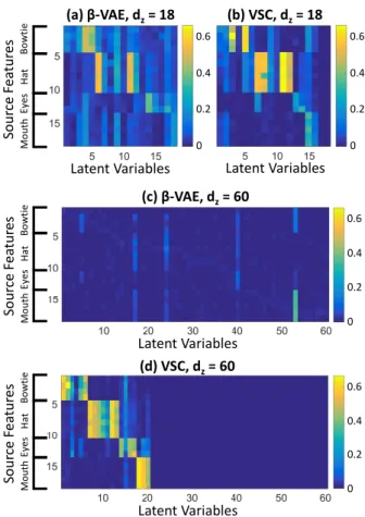
Both models are given neural networks of equal capac-ity. We then test features disentanglement with a test set of20,000new samples by computing the absolute value of the correlation between each source feature and each recovered latent variable. Additional details about these experiments can be found in supplementary D.2. Abso-lute value of correlation matrices for the two models are shown in figure 3. If the number of latent dimensions is chosen to match that of the generating features, the β-VAE displays appreciable correlation between the true attributes and the recovered latent variables. The VSC model displays higher correlation contrast and hence bet-ter disentanglement. This is due to the fact that VSC is able to model with its prior both the presence or absence of different features in different observations and their continuous variability, while aβ-VAE attempts to model the data only with continuous variables.
As shown in figure 3(c), in the situation where the num-ber of generating dimensions was assumed to be un-known, theβ-VAE did not recover latent variables that well correlate with each source feature.β-VAEs encour-age encoded data to be distributed as a univariate Gaus-sian distribution which is factorisable along all its latent space axis. This is effective in situations where the num-ber of latent variables is chosen to match fairly well the number of source features, as shown in figure 3(a), and even more so if such features are all present and contin-uously distributed in each example, as demonstrated by Higgins et al. (2017a). However, in a more general situa-tion, where data is described by different superpositions
(d) VSC, dz= 60 Latent Variables So ur ce Fea tu res Bowtie Hat Ey es Mo u th So u rc e Fea tu res Bowtie Hat Ey es Mo u th (c) β-VAE, dz= 60 Latent Variables So u rc e Fea tu res Bowtie Hat Ey es Mo u th
Latent Variables Latent Variables (a) β-VAE, dz= 18 (b) VSC, dz= 18 0 0.2 0.4 0.6 0 0.2 0.4 0.6 0 0.2 0.4 0.6 0 0.2 0.4 0.6
Figure 3: Absolute value of correlation between source features and latent variables for the Smiley data set. The x-axis indicates the index of the latent variable. Variables have been permuted to group dimensions that display the highest correlation with the same feature. Feature disen-tanglement is achieved if each latent variable correlates strongly with one source attribute but weakly with the re-maining ones thus leading to a block diagonal structure.
of features and their number is not known a priori, en-forcing a latent distribution that factorises along all axis does not result into good source features recovery; the model forces data to stretch along many more dimen-sions than it is necessary to describe it, dispersing the correlation with the true sources of variation.
Conversely, as shown in figure 3(d), the VSC model is able to disentangle well the different features groups. Because it is designed to model different combinations of features, it can activate or deactivate latent variables for each encoding according to the features recognised in each observation and it successfully disentangles each at-tribute in distinct sub-spaces with little interdependence, regardless of the choice of latent space dimensionality. The VSC model adjusted to a suitable number of latent variables needed to represent the data. In the matrix of figure 3(d), the zero columns correspond to collapsed
di-mensions where the latent variables were consistently in-active. Given60latent dimensions prior to training and no knowledge of the source dimensionality or sparsity, the model collapsed to 20 exploited dimensions to de-scribe data generated independently from18source vari-ables. The number of latent variables assigned to each feature group is also recovered with fairly good accu-racy, as the VSC correlation matrix in figure 3 presents a near-block diagonal structure. We also compare feature disentanglement with theβ-TCVAE (Gao et al., 2019) and its behaviour at increasing latent space dimensional-ity was found to be analogous to that of theβ−VAE. The correlation matrices from these experiments are shown in full in supplementary F.
It is not possible to quantify feature disentanglement in natural data, as the source features are not known. How-ever, similarly to Kim & Mnih (2018), we can qualita-tively examine the effect of changing single latent vari-ables on generated samples. To this end, we train a VSC model with 100,000 examples from the CelebA data set, encode examples from a test set, alter individu-ally exploited dimensions in the latent space and finindividu-ally generate samples from these altered latent vectors. We find that several of the dimensions exploited by the VSC model control interpretable aspects in the generated data, as shown in the examples of figure 4.
4.3 FEATURE ACTIVATION RECOVERY
The Spike probabilities retrieved when encoding an ob-servation can be interpreted as the probabilities of cer-tain recognised features being present or absent in a given sample. These activation patterns can be used to
Lighting position
Smile
Fringe
Figure 4: Examples are generated by altering individ-ual latent variables in a VSC model trained on the celebA data set. Individual latent variables control in-terpretable aspects of the generated images, i.e., inter-pretable sources of variation are aligned with the repre-sentation space axis.
investigate what features different objects are expected to have in common. As an example, we train two VSC models having60latent dimensions with the training sets from the Fashion-MNIST and UCI HAR data sets re-spectively, encode the entire test sets and examine the
T-shirt Trousers Jumpers Dresses Shirts Sandals Tops Shoes Bags Boots Latent Variables Cl as se s Up p er B ody Foo tw ear Fashion-MNIST Walking Walking Upstairs Laying Sitting Standing Walking Downstairs UCI HAR Act ivity In ac tivit y Cl as se s Latent Variables Cl as se s 10 20 30 40 50 60 10 20 30 40 50 60 1 0.2 0.4 0.6 0.8 0 0.2 0.4 0.6 0.8 0 1
Figure 5: Average Spike probability per class in (a) Fashion-MNIST and (b) UCI HAR. Black corresponds to0, or always inactive, and white to1, or always active. The Spike probabilities show the recovered features classes have in common. Objects that are similar, such as T-shirts and shirts in the Fashion-MNIST example, activate mostly the same latent dimensions, i.e., they can largely be described with the same features. More distinct objects, such as T-shirts and trousers, activate different latent dimensions, i.e., they exploit different features to express their variability.
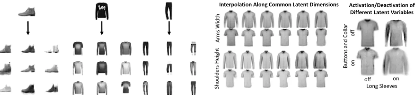
Figure 6: Generation conditioned on single observations with the VSC model. An object is encoded in the latent space and synthetic examples are then generated by sam-pling only along the activated latent dimensions. This makes it possible to generate a variety of objects that share the same features with the input object without any supervision.
average Spike probabilities per class recovered by the recognition model. Results are shown in figure 5. In the VSC latent space, similar classes present a high over-lap of active latent variables, while classes that are very different exploit different sets of latent dimensions to de-scribe their samples. These Spike variable activation pat-terns readily provide a visualisation of the similarity of different objects in terms of the factors of variation they are described by.
The capability of VSC to recover feature exploitation for a given observation can also be used to control gener-ation. For instance, it is possible to generate samples conditioned on a single object by exploring the subspace defined by the activated latent variables of such object. Figure 6 shows examples of images generated by encod-ing a sencod-ingle observation from Fashion-MNIST and sub-sequently sample the subspace defined by the resulting active dimensions. As shown in figure 6, the VSC model naturally provides a way of performing conditional gen-eration without the need for any supervision.
The VSC model can also be used to study the nature of the difference between objects through controlled gener-ation. Two objects may have some active latent variables in common, describing characteristics that they both re-tain, but that might have different values, and some that are different, describing features that they do not have in common. For instance, in figure 7, we consider the features of a T-shirt and a shirt taken from the Fashion-MNIST test set. The VSC latent variables for the two observations share some dimensions, which we individ-ually alter and generate from. Examples are shown on the left of figure 7. As shown, these dimensions control features the two objects have in common. Conversely, there are some latent dimensions that are active for one
Interpolation Along Common Latent Dimensions Activation/Deactivation of Different Latent Variables
B ut tons a nd C ol la r Long Sleeves off on of f on A rm s Wi dth Shoul der s He ig h t
Figure 7: Investigating the difference between two ob-jects with VSC. Single examples of a T-shirt and a shirt are encoded in the latent space. On the left, generations obtained by individually altering two latent dimensions which are active for both objects. On the right, gener-ations obtained by activating and deactivating latent di-mensions exploited by one object, but not the other.
observation, but not the other and vice versa. These di-mensions correspond to the recovered features the two objects do not share. The effects on generation of activat-ing and deactivatactivat-ing two of these for the T-shirt example are shown on the right of figure 7.
All of the controlled generation examples described above are carried out without any supervision, but sim-ply by examining and individually controlling the latent dimensions activated by single observation examples.
5
CONCLUSION
We present a new model to retrieve non-linear sparse rep-resentations of data through a variational auto-encoding approach. The proposed VSC model is capable of re-trieving and disentangling sources of variation from di-verse data, where attributes can be present and absent in different combinations and the total number of factors of variation and their occurrence is unknown a priori. The sparse representations also offer novel visualisation and generation capability, thanks to the ability to exam-ine and exploit latent variable activation. In defining the VSC model, we also contribute general components and methods that can be used to perform sparse probabilis-tic inference in different settings, such as an analyprobabilis-tical expression for the Spike and Slab KL divergence and a Spike pre-training strategy.
Acknowledgements:
F.T. acknowledges support from Amazon Research and EPSRC grant EP/M01326X/1, B.S.J. from EP-SRC grant EP/R018634/1, and R.M-S. EPEP-SRC grants EP/M01326X/1 and EP/R018634/1.
References
D. Anguita, A. Ghio, L. Oneto, X. Parra, and J. L Reyes-Ortiz. Human activity recognition on smartphones us-ing a multiclass hardware-friendly support vector ma-chine. InProceedings of the International Workshop
on Ambient Assisted Living, pp. 216–223. Springer,
2012.
Y. Bengio, A. Courville, and P. Vincent. Representation learning: A review and new perspectives.IEEE
Trans-actions on Pattern Analysis and Machine Intelligence,
pp. 1798–1828, 2013.
C. P. Burgess, I. Higgins, A. Pal, L. Matthey, N. Wat-ters, G. Desjardins, and A. Lerchner. Understanding disentangling inβ-VAE. arXiv:1804.03599, 2018. T. Q. Chen, X. Li, R.B. Grosse, and D.K. Duvenaud.
Isolating sources of disentanglement in variational au-toencoders. InProceedings of the Advances in
Neu-ral Information Processing Systems, pp. 2610–2620,
2018.
A. Cherian and S. Sra. Riemannian dictionary learning and sparse coding for positive definite matrices.IEEE Transactions on Neural Networks and Learning Sys-tems, 28(12):2859–2871, 2017.
Y. Gal. Uncertainty in deep learning. PhD thesis, Uni-versity of Cambridge, 2016.
S. Gao, R. Brekelmans, G.V. Steeg, and A. Galstyan. Auto-encoding total correlation explanation. In Pro-ceedings of the International Conference on Artificial
Intelligence and Statistics, 2019.
I. Goodfellow, A. Courville, and Y. Bengio. Large-scale feature learning with Spike-and-Slab sparse coding. In
Proceedings of the International Conference on
Ma-chine Learning, 2012.
I. Higgins, L Matthey, A Pal, C Burgess, X Glorot, M. Botvinick, S Mohamed, and A Lerchner. β-VAE: Learning basic visual concepts with a constrained vari-ational framework. InProceedings of the International
Conference on Learning Representations, 2017a.
I. Higgins, L. Matthey, A. Pal, C. Burgess, X. Glorot, M. Botvinick, S. Mohamed, and A. Lerchner.β-VAE: Learning basic visual concepts with a constrained vari-ational framework. InProceedings of the International
Conference on Learning Representations, 2017b.
J. Ho, Y. Xie, and B. Vemuri. On a nonlinear generaliza-tion of sparse coding and dicgeneraliza-tionary learning. In Pro-ceedings of the International Conference on Machine
Learning, pp. 1480–1488, 2013.
H. Kim and A. Mnih. Disentangling by factorising. In
Proceedings of the International Conference on
Ma-chine Learning, pp. 2649–2658, 2018.
D. P. Kingma and M. Welling. Auto-encoding variational bayes. InProceedings of the International Conference
on Learning Representations, 2013.
H. Lee, A. Battle, R. Raina, and A. Y. Ng. Efficient sparse coding algorithms. Neural Computation, pp. 801–808, 2007.
C. J. Maddison, A. Mnih, and Y. W. Teh. The Concrete distribution: A continuous relaxation of discrete ran-dom variables. In Proceedings of the International
Conference on Learning Representations, 2017.
E. Mathieu, T. Rainforth, N. Siddharth, and Y. W. Teh. Disentangling disentanglement in variational autoen-coders. In Proceedings of the International
Confer-ence on Machine Learning, pp. 4402–4412, 2019.
T. J. Mitchell and J. J. Beauchamp. Bayesian variable selection in linear regression.Journal of the American
Statistical Association, 83(404):1023–1032, 1988.
E. Nalisnick and P. Smyth. Stick-breaking variational au-toencoders. InProceedings of the International
Con-ference on Learning Representations, 2017.
B. A. Olshausen and D. J. Field. Emergence of simple-cell receptive field properties by learning a sparse code for natural images. Nature, 381(6583):607, 1996a. B. A. Olshausen and D. J. Field. Natural image statistics
and efficient coding.Network: Computation in Neural
Systems, 7(2):333–339, 1996b.
B. A. Olshausen and D. J. Field. Sparse coding of sen-sory inputs. Current opinion in neurobiology, 14(4): 481–487, 2004.
Y. Pu, Z. Gan, R. Henao, X. Yuan, C. Li, A. Stevens, and L. Carin. Variational autoencoder for deep learning of images, labels and captions. InProceedings of the
Advances in Neural Information Processing Systems,
2016.
D. J. Rezende, S. Mohamed, and D. Wierstra. Stochastic backpropagation and approximate inference in deep generative models. InProceedings of the International
Conference on Machine Learning, 2014.
J. T. Rolfe. Discrete variational autoencoders. In Pro-ceedings of the International Conference on Learning
R. Singh, J. Ling, and F. Doshi-Velez. Structured Vari-ational Autoencoders for the Beta-Bernoulli Process.
InProceedings of the Advances in Neural Information
Processing Systems, 2017.
C. K. Sønderby, T. Raiko, L. Maaløe, S. K. Sønderby, and O. Winther. How to train deep variational au-toencoders and probabilistic ladder networks. In Pro-ceedings of the International Conference on Machine
Learning, 2016.
M. K. Titsias and M. L´azaro-Gredilla. Spike and Slab variational inference for multi-task and multiple ker-nel learning. InProceedings of the Advances in
Neu-ral Information Processing Systems, pp. 2339–2347,
2011.
J. M. Tomczak and M. Welling. VAE with a
Vamp-Prior. In Proceedings of the International
Confer-ence on Artificial IntelligConfer-ence and Statistics, pp. 1214–
1223, 2018.
A. van den Oord, O. Vinyals, and K. Koray. Neural dis-crete representation learning. InProceedings of
Ad-vances in Neural Information Processing Systems, pp.
6306–6315, 2017.
H. Xiao, K. Rasul, and R. Vollgraf. Fashion-MNIST: a novel image dataset for benchmarking machine learn-ing algorithms.arXiv:1708.07747, 2017.
S. Yeung, A. Kannan, Y. Dauphin, and L. Fei-Fei. Tack-ling over-pruning in variational autoencoders. Inter-national Conference on Machine Learning: Workshop
Variational Sparse Coding - Supplementary material
A
DETAILS OF THE VSC MODEL
We describe here the details of the VSC model and the architecture of all the neural networks the VSC model is constructed with.
A.1 LIKELIHOOD FUNCTION
The likelihood functionp(x|zi)is composed of a neural network which takes as input a latent variablezi ∈ RJ×1
and outputs the meanµi ∈ RM×1 and log variancelog(σ2i) ∈ RM×1. The log likelihood of a samplexi is then
computed evaluating the log probability density assigned toxiby a Gaussian having meanµiand standard deviation
σi. In our experiments we use a one hidden layer fully connected neural network for all experiments. The hidden layer
between the latent space and the observation space was chosen to have between1,000and3,000units, depending on the experimental settings.
A.2 RECOGNITION MODEL
The recognition modelp(z|xi)is composed of a neural network which takes as input an observationxi ∈RM×1and
outputs the meanµz,i ∈ RJ×1, the log variancelog(σz,i2 ) ∈RJ×1and the log Spike probabilities vectorlog(γi)∈
RJ×1. The elements ofγineed to be constrained between0and1, therefore, other than usinglog(γi)as output, which
ensuresγi>0, we employ a ReLU non-linearity at this output of the neural network as follows
log(γi) =−ReLU(−vout,i),
wherevout,iis output to the same standard neural network that outputsµz,iandlog(σ2z,i). This ensures thatγi <1.
Samples in the latent spacezi,lcan then be drawn as detailed in supplementary B.1. The structure of the neural network
is analogous to that of the likelihood function, with one hidden layer of1,000to3,000units between the observation space and the latent space.
A.3 SELECTION FUNCTION
The selection functionCω(xi)is composed of a one layer neural network which takes observationsxi as input and
returns a vector with the dimensionaliy equal to the number of possible pseudo-inputsu. The output is normalised to unitary sum, then, to encourage the selection of a single pseudo-input while retaining differentiability, the resulting vector is passed through a scaled and displaced Sigmoid function as follows
u∗=S(a(u−b)),
whereu∗is the output selection vector,ais chosen to be equal to60in our experiments andbis chosen to be0.5. The ELBO KL divergence for a given inputxi is then computed as a weighted sum of the KL divergences of the
recognition model with each pseudo-input encoding, where the weights are the elements ofu∗.
B
SPIKE AND SLAB DRAWS REPARAMETRISATION
B.1 REPARAMETRISATION OF THE DRAWS
The drawszi,lare computed as follows
whereindicates an element wise product. The functionT(yi,l)is in principle a step function centered at zero,
however, in order to maintain differentiability, we employ a scaled Sigmoid function T(y) = S(cy). In the limit c → ∞,S(cy)tends to the true binary mapping. In practice, the value ofc needs to be small enough to provide stability of the gradient ascent. In our implementation we employ a warm-up strategy to gradually increase the value ofcduring training.
B.2 SPIKE VARIABLE REPARAMETRISATION
We report here a detailed description of the Spike variable reparametrisation, similar to the relaxation of discrete variables in Maddison et al. (2017) and Rolfe (2017). Our aim is to find a functionf(ηl,j, γi,j)such that a binary
variablewi,l,j ∼p(wi,l,j)drawn from the discrete distributionp(wi,l,j = 1) =γi,j, p(wi,l,j = 0) = (1−γi,j)can be
expressed aswi,l,j =f(ηl,j, γl,j), whereηl,j is some noise variable drawn from a distribution which does not depend
onγi,j.
The function of choicef(ηl,j, γi,j) should ideally only take values1 and0, as these are the only values ofwi,l,j
permitted byp(wi,l,j). Furthermore, the probabilities ofwi,l,jbeing1or0are linear inγi,j, therefore the distribution
of the noise variableηi,jshould have evenly distributed mass. The simplest function which satisfy these conditions
and yields our reparametrisation is then a step functionf(ηl,j, γi,j) =T(ηl,j−p(wi,l,j = 0)) =T(ηl,j −1 +γi,j)
whereηl,jis uniformly distributed andT(y)is the following step function
T(y) =
(
1, ify≥0. 0, ify <0.
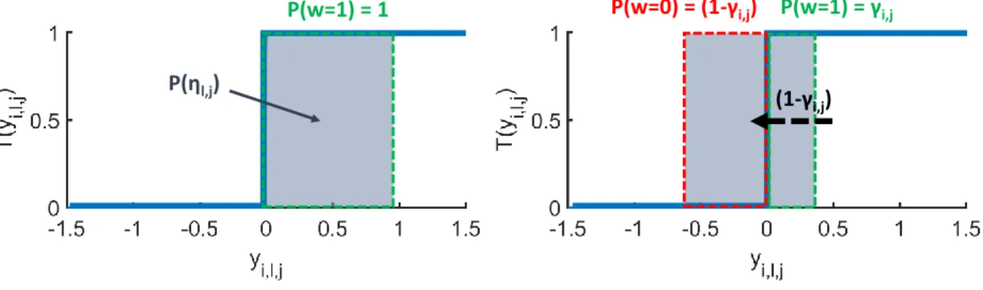
An illustration of this reparametrisation is shown in figure 8.
P(η
l,j)
P(w=0) = (1-
γ
i,j)
P(w=1) = 1
P(w=1) =
γ
i,j(1-
γ
i,j)
Figure 8: Schematic representation of the reparametrisation of the Spike variable. The variableyi,l,j is drawn in
the range covered by the grey square with probability proportional to its height. On the left, for a spike probability γi,j= 1, the variableyi,l,jis drawn to always be greater than zero and the Spike variablewi,l,jis always one. On the
right, for an arbitraryγi,j, the probability density ofyi,l,jis displaced to the left by1−γi,jandyi,l,j has probability
γi,jof being≥0, in which casewi,l,jis one, and probability1−γi,jof being<0, in which casewi,l,jis zero.
The functionT(yi,l,j)is not differentiable, therefore we approximate it with a scaled SigmoidS(cyi,l,j), wherecis a
real positive constant. In our implementation, we gradually increasecfrom50to200during training to achieve good approximations without making convergence unstable.
C
DERIVATION OF THE SPIKE AND SLAB KL DIVERGENCE
We report here a detailed derivation of the KL divergence between two Spike and Slab distributions shown in equation 6. The KL divergence can be separated into four cross entropy components in each latent dimension
DKL(qφ(z|xi)||qφ(z|xu∗)) = Z qφ(z|xi)(logqφ(z|xi)−logqφ(z|xu∗))dz = J X j −γi,j Z
N(zi,j;µz,i,j, σz,i,j2 ) log
γu∗,jN(zi,j;µz,u∗,j, σz,u2 ∗,j) + (1−γu∗,j)δ(zj)dzj
| {z }
1 −(1−γi,j)
Z
δ(zi,j) logγu∗,jN(zi,j;µz,u∗,j, σz,u2 ∗,j) + (1−γu∗,j)δ(zj)dzj
| {z }
2
+γi,j Z
N(zi,j;µz,i,j, σz,i,j2 ) log
γi,jN(zi,j;µz,i,j, σz,i,j2 ) + (1−γi,j)δ(zi,j) dzj | {z } 3 + (1−γi,j) Z δ(zi,j) log
γi,jN(zi,j;µz,i,j, σz,i,j2 ) + (1−γi,j)δ(zi,j) dzj | {z } 4 .
1 and 3 are of a similar form; the cross entropy between a Gaussian and a discrete mixture distributions. These components reduce to the corresponding Gaussian-Gaussian entropy terms, as the point mass contributions vanish. In fact, for any finite density distributionsf(zj)andg(zj), the point mass contribution to the cross entropy between
f(zj)and a discrete mixtureh(zj) =αg(zj) + (1−α)δ(zj−c)is infinitesimal. The proof is as follows; the cross
entropy between the functionsf(zj)andh(zj)is Z
f(zj) log [αg(zj) + (1−α)δ(zj−c)]dzj.
We can split this integral in two components over two different domains, the first in the region wherezj 6=cand the
second in the region wherezj =c. By using a Dirac Delta function, the first component can be expressed as follows Z zj6=c f(zj) log [αg(zj) + (1−α)δ(zj−c)]dzj= Z zj6=c f(zj) log [αg(zj)]dzj= Z 1−δ(zj−c) δ(0) f(zj) log [αg(zj)]dzj,
where from the first to the second line we can ignore the component containingδ(zj −c), as the domain does not
includezj = c. We then use a coefficient which is zero atzj = cand one otherwise to write the integral over the
whole domain ofzj. Similarly, we can write the term in the domainzj=cas Z zj=c f(zj) log [αg(zj) + (1−α)δ(zj−c)]dzj = Z δ(z j−c) δ(0) f(zj) log [αg(zj) + (1−α)δ(zj−c)]dzj,
Z f(zj) log [αg(zj) + (1−α)δ(zj−c)]dzj = Z 1−δ(zj−c) δ(0) f(zj) log [αg(zj)] + +δ(zj−c) δ(0) f(zj) log [αg(zj) + (1−α)δ(zj−c)] dzj.
Rearranging to gather the terms inδ(zj−c)/δ(0)we get
Z f(zj) log [αg(zj)]dzj+ Z δ(z j−c) δ(0) f(zj) log [αg(zj) + (1−α)δ(zj−c)]−f(zj) log [αg(zj)] dzj = Z f(zj) log [αg(zj)]dzj+ Z δ(z j−c) δ(0) f(zj) log αg(z j) + (1−α)δ(zj−c) αg(zj) dzj.
Simplifying the argument of the second logarithm and solving the second integral we get
Z f(zj) log [αg(zj) + (1−α)δ(zj−c)]dzj = Z f(zj) log [αg(zj)]dzj+ lim u→∞ f(c) u log(1 + 1−α α u g(c)),
where the second term tends to zero, leaving the cross entropy betweenf(zj)andαg(zj). Applying this result to 1
and 3 we obtain the following
3 − 1 =γi,j
Z
N(zi,j;µz,i,j, σz,i,j2 ) log
γi,jN(zi,j;µz,i,j, σ2z,i,j)
− N(zi,j;µz,i,j, σ2z,i,j) log
γu∗,jN(zi,j;µz,u∗,j, σ2z,u∗,j)
dzj
=γi,j Z
N(zi,j;µz,i,j, σz,i,j2 ) log "
γi,jN(zi,j;µz,i,j, σ2z,i,j)
γu∗,jN(zi,j;µz,u∗,j, σz,u2 ∗,j)
#
dzj
=γi,jDKL N(zi,j;µz,i,j, σ2z,i,j) || N(zi,j;µz,u∗,j, σz,u2 ∗,j)+γi,jlog
γ i,j γu∗,j . (8)
The KL divergenceDKL N(zi,j;µz,i,j, σz,i,j2 ) || N(zi,j;µz,u∗,j, σ2z,u∗,j)
is the Gaussian-Gaussian KL divergence and has a simple analytic form:
DKL N(zi,j;µz,i,j, σz,i,j2 ) || N(zi,j;µz,u∗,j, σz,u2 ∗,j)= log σz,u∗,j
σz,i,j
+σz,i,j+ (µz,i,j−µz,u∗,j)
2
2σz,u∗,j
−1
2 (9)
2 and 4 take the form of the cross entropy between a Dirac Delta function and a discrete mixture distribution. In this case, instead, the continuous density contributions vanish:
4 − 2 = (1−γi,j) Z
δ(zi,j) log
γi,jN(zi,j;µz,i,j, σz,i,j2 ) + (1−γi,j)δ(zi,j)
−log
γu∗,jN(zi,j;µz,u∗,j, σz,u2 ∗,j) + (1−γu∗,j)δ(zi,j) dzj
= lim
u→∞(1−γi,j) log "
γi,jN(0;µz,i,j, σz,i,j2 ) + (1−γi,j)u
γu∗,jN(0;µz,u∗,j, σ2 z,u∗,j) + (1−γu∗,j)u # = (1−γi,j) log 1−γ i,j 1−γu∗,j . (10)
Substituting the results of equations 8, 9 and 10 into equation 8, we obtain the KL divergence between two general Spike and Slab distributions
DKL(qφ(z|xi)||qφ(z|xu∗)) = J X j 3 − 1 + 4 − 2 = J X j γi,jlog σz,u∗,j σz,i,j
+σz,i,j+ (µz,i,j−µz,u∗,j)
2 2σz,u∗,j −1 2 | {z } Slab KL Divergence + (1−γi,j) log 1−γ i,j 1−γu∗,j +γi,jlog γ i,j γu∗,j | {z } Spike KL Divergence .
This prior term presents two components. The first is the negative KL divergence between the distributions of the Slab variables, multiplied by the probability ofzi,j being non-zeroγi,j. The second term is the negative KL divergence
between the distributions of the Spike variables. We find of particular interest that by computing the KL divergence analytically we recover a linear combination of the Spike and Slab components divergences.
D
DETAILS OF THE EXPERIMENTS
D.1 ELBO EVALUATION EXPERIMENTAL DETAILS
For the ELBO evaluation experiments, we train identical VSC models for the Fashion-MNIST and UCI-HAR datasets, with the exception of the first layer in the recognition model and the last layer in the likelihood function, as the two data sets have different dimensionality (784 and 561 respectively). The likelihood function takes as input of a fully connected network a latent variablezi and maps it to a first deterministic layer of3,000dimensions. Two separate
fully connected network then map this layer to the observation space meanµand log variancelog(σ2)respectively. The recognition model takes as input of a fully connected network an observationxiand maps it to a first deterministic
layer of3,000dimensions. Three separate fully connected networks then map this layer to the latent space meanµz,i,
log variancelog(σ2
z,i)and spike probabilitiesγirespectively. The selection functionu∗ =Cω(x)is composed of a
single fully connected layer (linear matrix and ReLu non-linearity) taking as input observationsxiand outputting a
selection vector, as described in supplementary A.3. The total number of pseudo-inputs was set to20.
The models were then trained with the ADAM optimiser in Tensorflow, with a batch size of500. The spike pre-training, carried out as described in section 3.4, was performed over15,000iterations withλ= 0.λwas then linearly increased between0and1over 5,000iterations. During this phase, the initial training rate was set to10−3. The model is then trained further for50,000iterations and an initial training rate of10−4.
Theβ-VAE was trained with as an identical structure as possible; The likelihood function was identical to that of the VSC and the recognition model was given the same structure, a side of the fact that there is no mapping to a Spike variable. Theβ-VAE was trained for70,000iterations with the same batch size and an initial training rate of
10−4. Each data point in figure 1 is obtained by performing the same experiment five times with different random initialisation and seeds. the points are obtained as the means and the error bars as the standard deviations of the results.
D.2 FEATURES DISENTANGLEMENT EXPERIMENTAL DETAILS
For the feature disentanglement experiments using the Smiley sparse data set we use a VSC andβ-VAE identical to those used in the Fashion-MNIST ELBO evaluation, as the two types of data have the same dimensionality. The VSC model is trained with the ADAM optimiser over a total of200,000iterations with a batch size of500. 50,000
iterations are dedicated to pre-training, withλ= 0, thenλis linearly increased to1over10,000iterations and the model is then trained withλ= 1for the remaining training duration. During the first pre-training60,000iterations, the optimiser is given a step size of5×10−4, which is then decreased to5×10−5for the rest of training. Theβ-VAE was given analogous structure and was trained over200,000iterations and a step size of5×10−5. The value ofβ
was cross validated between1and50at increasing steps between1and8and the model giving the best correlation contrast in the matrices shown was chosen.
The results obtained with the CelebA data set were obtained with the same VSC architecture described above, with the only differences that the observation space is of3072dimensions (the CelebA examples were down-sampled to
32×32) and, due to this higher dimensionality, the latent space was given300dimensions. The model was trained with the same training parameters described above. However, the total number of iterations was extended to500,000, maintaining the same Spike pre-training procedure.
D.3 FEATURES ACTIVATION EXPERIMENTAL DETAIL
The matrices of figure 6 were obtained from the exact models trained for the ELBO evaluations at a prior sparsity ofα= 0.01. The images shown for the examples of conditional sampling in figure 6 and controlled continuous and discrete interpolation of figure 7 are also generated from the same VSC model, trained with the Fashion-MNIST data set.
E
SMILEY DATA SET DETAILS
The Smiley sparse data set is composed of32×32binary images of automatically generated smileys. the base of every example is a centered filled circle10pixels in radius. Each example is then generated with a sparse superposition of4
attributes, each defined by a variable number of features. The attribute are assigned a fixed probability of being present or absent in each example. The attributes are the following:
• Eyes- The eyes are added as two symmetric circular holes in the circular head and are determined by3variables: vertical position, horizontal separation and radius. If eyes are active, each of these features is drawn from a normal distribution with standard deviation of0.5pixels.
• Mouth- The mouth is added as a central horizontal rectangular hole and two smaller horizontal rectangular holes
at its side at the bottom of the head. It is determined by5variables: vertical position, horizontal position, vertical width, horizontal length and vertical position of side holes. If mouth is active, each of these features is drawn from a normal distribution with standard deviation of0.5pixels.
• Hat - The hat is added as a larger rectangle above the smiley’s head and a smaller rectangle above it. It is determined by6variables: vertical and horizontal position, height and width of larger rectangle, height and width of smaller rectangle. If hat is active, features are drawn from normal distributions with the following standard deviations:0.5pixels for the two position variables,1pixels for the vertical position of the larger rectangle,1.5
pixels for the horizontal position of the larger rectangle,0.5pixels for the vertical position of the smaller rectangle and1pixels for the horizontal position of the smaller rectangle.
• Bowtie- The Bowtie is inserted by adding an image of two triangles connected at a corner at the bottom of
the smiley’s head. It is determined by 4 variables: vertical position, horizontal position, vertical width and horizontal length. If mouth is active, these features are drawn from normal distributions with the following standard deviations: 0.5pixels for vertical position,0.25pixels for horizontal position,1pixels for height, and
All of the aforementioned standard deviations and other parameters can be altered in the generating code to make dif-ferent variations of the smiley sparse data set. THe dataset used in our experiments was generated with the parameters detailed above and an attribute presence probability of0.5.
F
ADDITIONAL FEATURE DISENTANGLEMENT RESULTS
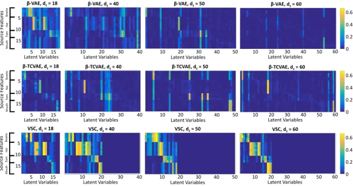
We show in figure 9 absolute value of correlation matrices analogous to those shown in figure 3, but forβ-VAE, β-TCVAE, and VSC for different choices of latent space dimensionalitydz. As the number of latent dimensions
in-creases, the correlation between ground-truth features and latent variables recovered with theβ-VAE and theβ-TCVAE decreases, as these unsupervised disentanglement models force to disperse the18original generating variables into an increasingly larger number of factors of variation. Conversely, the VSC model maintains good feature disentanglement regardless of latent dimensionality, as the correlation contrast remails strong in all experiments. Furthermore, VSC consistently activates a number of variables which is close to the true number of sources of variation, both in total and for each attribute (zero column indicate latent variables that were never used), as the correlation matrices all present a close to square matrix with block diagonal structure.
So u rc e Fea tu res Bow ti e Hat Ey es M o u th Latent Variables β-VAE, dz= 18 β-VAE, dz= 40
Latent Variables Latent Variables
β-VAE, dz= 50 β-VAE, dz= 60 Latent Variables 5 10 15 5 10 15 10 20 30 40 10 20 30 40 50 10 20 30 40 50 60 So u rc e Fea tu res Bo w ti e Hat Ey es M o u th Latent Variables β-TCVAE, dz= 18 β-TCVAE, dz= 40
Latent Variables Latent Variables
β-TCVAE, dz= 50 β-TCVAE, dz= 60 Latent Variables 5 10 15 5 10 15 10 20 30 40 10 20 30 40 50 10 20 30 40 50 60 So u rc e Fea tu res Bow ti e Hat Ey es M o u th Latent Variables VSC, dz= 18 VSC, dz= 40
Latent Variables Latent Variables
VSC, dz= 50 VSC, dz= 60 Latent Variables 5 10 15 5 10 15 10 20 30 40 10 20 30 40 50 10 20 30 40 50 60 0.2 0 0.4 0.6 0.2 0 0.4 0.6 0.2 0 0.4 0.6
Figure 9: Absolute value of correlation between source features and recovered latent variables with the Smiley sparse data set for multiple choices of latent space dimensionality. While theβ-VAE and the β-TCVAE gradually loses their feature disentanglement properties as the number of dimensions is made increasingly different from the number of true sources of variation, the VSC maintains strong disentanglement properties, independently of the choice of dimensionality.
Variational Sparse Coding - Supplementary material
A
DETAILS OF THE VSC MODEL
We describe here the details of the VSC model and the architecture of all the neural networks the VSC model is constructed with.
A.1 LIKELIHOOD FUNCTION
The likelihood functionp(x|zi)is composed of a neural network which takes as input a latent variablezi ∈ RJ×1
and outputs the meanµi ∈ RM×1 and log variancelog(σ2i) ∈ RM×1. The log likelihood of a samplexi is then
computed evaluating the log probability density assigned toxiby a Gaussian having meanµiand standard deviation
σi. In our experiments we use a one hidden layer fully connected neural network for all experiments. The hidden layer
between the latent space and the observation space was chosen to have between1,000and3,000units, depending on the experimental settings.
A.2 RECOGNITION MODEL
The recognition modelp(z|xi)is composed of a neural network which takes as input an observationxi ∈RM×1and
outputs the meanµz,i ∈ RJ×1, the log variancelog(σz,i2 ) ∈RJ×1and the log Spike probabilities vectorlog(γi)∈
RJ×1. The elements ofγineed to be constrained between0and1, therefore, other than usinglog(γi)as output, which
ensuresγi>0, we employ a ReLU non-linearity at this output of the neural network as follows
log(γi) =−ReLU(−vout,i),
wherevout,iis output to the same standard neural network that outputsµz,iandlog(σ2z,i). This ensures thatγi <1.
Samples in the latent spacezi,lcan then be drawn as detailed in supplementary B.1. The structure of the neural network
is analogous to that of the likelihood function, with one hidden layer of1,000to3,000units between the observation space and the latent space.
A.3 SELECTION FUNCTION
The selection functionCω(xi)is composed of a one layer neural network which takes observationsxi as input and
returns a vector with the dimensionaliy equal to the number of possible pseudo-inputsu. The output is normalised to unitary sum, then, to encourage the selection of a single pseudo-input while retaining differentiability, the resulting vector is passed through a scaled and displaced Sigmoid function as follows
u∗=S(a(u−b)),
whereu∗is the output selection vector,ais chosen to be equal to60in our experiments andbis chosen to be0.5. The ELBO KL divergence for a given inputxi is then computed as a weighted sum of the KL divergences of the
recognition model with each pseudo-input encoding, where the weights are the elements ofu∗.
B
SPIKE AND SLAB DRAWS REPARAMETRISATION
B.1 REPARAMETRISATION OF THE DRAWS
The drawszi,lare computed as follows
whereindicates an element wise product. The functionT(yi,l)is in principle a step function centered at zero,
however, in order to maintain differentiability, we employ a scaled Sigmoid function T(y) = S(cy). In the limit c → ∞,S(cy)tends to the true binary mapping. In practice, the value ofc needs to be small enough to provide stability of the gradient ascent. In our implementation we employ a warm-up strategy to gradually increase the value ofcduring training.
B.2 SPIKE VARIABLE REPARAMETRISATION
We report here a detailed description of the Spike variable reparametrisation, similar to the relaxation of discrete variables in Maddison et al. (2017) and Rolfe (2017). Our aim is to find a functionf(ηl,j, γi,j)such that a binary
variablewi,l,j ∼p(wi,l,j)drawn from the discrete distributionp(wi,l,j = 1) =γi,j, p(wi,l,j = 0) = (1−γi,j)can be
expressed aswi,l,j =f(ηl,j, γl,j), whereηl,j is some noise variable drawn from a distribution which does not depend
onγi,j.
The function of choicef(ηl,j, γi,j) should ideally only take values1 and0, as these are the only values ofwi,l,j
permitted byp(wi,l,j). Furthermore, the probabilities ofwi,l,jbeing1or0are linear inγi,j, therefore the distribution
of the noise variableηi,jshould have evenly distributed mass. The simplest function which satisfy these conditions
and yields our reparametrisation is then a step functionf(ηl,j, γi,j) =T(ηl,j−p(wi,l,j = 0)) =T(ηl,j −1 +γi,j)
whereηl,jis uniformly distributed andT(y)is the following step function
T(y) =
(
1, ify≥0. 0, ify <0.
An illustration of this reparametrisation is shown in figure 8.
P(η
l,j)
P(w=0) = (1-
γ
i,j)
P(w=1) = 1
P(w=1) =
γ
i,j(1-
γ
i,j)
Figure 8: Schematic representation of the reparametrisation of the Spike variable. The variableyi,l,j is drawn in
the range covered by the grey square with probability proportional to its height. On the left, for a spike probability γi,j= 1, the variableyi,l,jis drawn to always be greater than zero and the Spike variablewi,l,jis always one. On the
right, for an arbitraryγi,j, the probability density ofyi,l,jis displaced to the left by1−γi,jandyi,l,j has probability
γi,jof being≥0, in which casewi,l,jis one, and probability1−γi,jof being<0, in which casewi,l,jis zero.
The functionT(yi,l,j)is not differentiable, therefore we approximate it with a scaled SigmoidS(cyi,l,j), wherecis a
real positive constant. In our implementation, we gradually increasecfrom50to200during training to achieve good approximations without making convergence unstable.