Any correspondence concerning this service should be sent
to the repository administrator: [email protected]
This is an author’s version published in:
http://oatao.univ-toulouse.fr/22365
Official URL
DOI : https://doi.org/10.1109/ICASSP.2018.8462197
Open Archive Toulouse Archive Ouverte
OATAO is an open access repository that collects the work of Toulouse
researchers and makes it freely available over the web where possible
To cite this version: Lagrange, Adrien and Fauvel, Mathieu and May,
Stéphane and Dobigeon, Nicolas A Bayesian model for joint unmixing and
robust classification of hyperspectral image. (2018) In: IEEE International
Conference on Acoustics, Speech, and Signal Processing (ICASSP 2018),
15 April 2018 - 20 April 2018 (Calgary, Canada).
A
BAYESIAN
MODEL
FOR
JOINT
UNMIXING
AND
ROBUST
CLASSIFICATION
OF
HYPERSPECTRAL
IMAGES
Adrien Lagrange
⋆Mathieu Fauvel
†St´ephane May
⋄Nicolas Dobigeon
⋆ ⋆University of Toulouse, IRIT/INP-ENSEEIHT, Toulouse, France
†
University of Toulouse, INP-ENSAT, UMR 1201 DYNAFOR, France,
⋄Centre National d’ ´
Etudes Spatiales (CNES), Toulouse, France
firsname.name@
{
enseeiht,ensat,cnes,enseeiht
}
.fr
ABSTRACT
Supervised classification and spectral unmixing are two methods to extract information from hyperspectral images. However, despite their complementarity, they have been scarcely considered jointly. This paper presents a new hierarchical Bayesian model to perform simultaneously both analysis in order to ensure that they benefit from each other. A linear mixture model is proposed to described the pixel measurements. Then a clustering is performed to identify groups of statistically similar abundance vectors. A Markov random field (MRF) is used as prior for the corresponding cluster labels. It pro-motes a spatial regularization through a Potts-Markov potential and also includes a local potential induced by the classification. Finally, the classification exploits a set of possibly corrupted labeled data provided by the end-user. Model parameters are estimated thanks to a Markov chain Monte Carlo (MCMC) algorithm. The interest of the proposed model is illustrated on synthetic and real data.
Index Terms— Bayesian model, Markov random Field, super-vised learning, image interpretation.
1. INTRODUCTION
Hyperspectral images are mainly interpreted via two widely used techniques, namely spectral unmixing (SU) and classification. SU aims at retrieving elementary components (referred to as endmem-bers) present in the image and the corresponding proportions within each pixel [1]. Conversely, classification assigns a unique label to each pixel using a predetermined nomenclature [2]. Both analysis own distinct advantages making them complementary. In particular, unmixing is an unsupervised subpixel analysis relying on physical descriptions of the observations [1, 3, 4]. To the contrary, supervised classification provides a semantic description of the hyperspectral image relying on external labeled data. Classification methods are extensively used to interpret remote sensing images and in particular hyperspectral images because of the multitude of available methods and the quality of their results [5–8]. Despite its potential interest in hyperspectral image analysis, the joint exploitation of the high-level (classification) and low-level (unmixing) approaches has been barely proposed [9, 10]. This paper proposes to fill this gap.
In [11], the authors proposed a Bayesian model as well as a corresponding algorithm to perform unmixing and spatial cluster-ing accordcluster-ing to the homogeneity of abundance vectors, which is a property also exploited recently in [12]. This paper extends this approach to handle the availability of a set of labeled data, akin to any conventional supervised framework which allows end-user to provide a set of labeled pixels. More precisely, the spectral-spatial
Par of this work has been supported Centre National d’ ´Etudes Spatiales (CNES) and Occitanie region.
clustering proposed in [11] is enriched to be also informed by the classification step. Moreover, since the classification step is recip-rocally informed by the clustering, this model allows errors in the ground-truth labels to be identified and corrected. Indeed, label mis-takes in user-provided labeled data is a well known issue when con-ducting supervised classification since they can impair the training process [13, 14]. By exploiting both labeled data and clustering, the robustness to labeling errors of the obtained classifier is improved, as illustrated in [15]. The resulting Bayesian model allows abundance vectors, clustering label and classification labels to be estimated si-multaneously. Consequently, the proposed algorithm produces a hi-erarchical description of the hyperspectral image in terms of unmix-ing, spectral-spatial segmentation and thematic classification.
The paper is organized as follows. Section 2 presents the model and more particularly develops the strategy to handle the unmixing, clustering and classification tasks jointly. A Markov chain Monte Carlo (MCMC) method is derived in Section 3 to sample according to the posterior of interest. Section 4 shows the results obtained on synthetic and real data. Conclusion is reported in Section 5.
2. FROM UNMIXING TO CLASSIFICATION 2.1. Problem statement
This work aims at performing the unmixing and classification of an hyperspectral image composed ofP pixel spectrayp ∈ RD (p ∈ P , {1, . . . , P}) which are measured inDspectral bands. TheRendmembersM= [m1, . . . ,mR]associated to elementary components of the mixing are assumed to be known. Two main quantities will be estimated: an abundance mapA= [a1, . . . ,aP] and a classification mapω = [ω1, . . . , ωP], whereapis the abun-dance vector associated to thepth pixel andωp∈ J ,{1, . . . , J}
is the classification label relating this pixel to a particular semantic class, withJthe number of classes. Each pixel is also characterized by a cluster labelzp ∈ K , {1, . . . , K}assigning this pixel to a group of homogeneous pixels. To reflect possible heterogeneity of the semantic class, each class is assumed to contain one or several clusters. Within a traditional supervised classification context, a par-tial ground-truth map of the image is provided as a training set. For-mally, a subset of thePpixels is assigned class labelscp∈ J. These labels are assumed to be potentially corrupted, e.g., due to some mis-classification by the end-user. In the following,L ⊂ Pstands for the set of indexes of this subset of labeled pixels and, conversely,
U = P\Ldenotes the set of indexes of the remaining (i.e., non-labeled) pixels. The hierarchical Bayesian model described hereafter is derived to perform the low-level (e.g., unmixing) and high-level (e.g., classification) tasks jointly, while simultaneously exploiting the high-level external informationcL ,{cp, p∈ L}. This model,
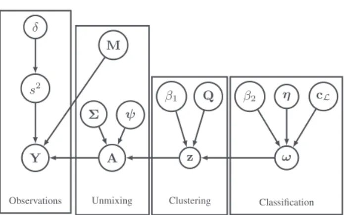
Y s2 δ M A Σ ψ z β1 Q ω β2 η cL
Observations Unmixing Clustering Classification
Fig. 1: Directed acyclic graph of the proposed model.
2.2. Bayesian hierarchical model
Mixing model – Following the conventional linear mixing model [1], each pixel of the observed hyperspectral image is described as a linear combination ofRendmembers corrupted by an additive noise
yp=Map+np (1)
wherenpis the noise associated to thepth pixel, assumed to be white and Gaussian, i.e.,np|s2 ∼ N(0D, s2ID), withID theD×D identity matrix and0DtheD-dimensional zero vector. It is worth noting that the proposed model can be easily adapted to handle non-whiteness or even non-Gaussian noises. Following the approach pro-posed by [11], a conjugate inverse-gamma distribution and a non-informative Jeffreys prior are used as a prior distributions for the noise variances2and the associated hyperparameter
s2|δ∼ IG(1, δ), p(δ)∝ 1
δ✶R+(δ) (2) where∝means proportional to and✶R+(·)is the indicator function
onR+. These choices ensure a straightforward estimation of the noise parameters. The observation model is then complemented by clustering and classification models described in the following sections.
Clustering model – As a bridge between the low-level task (i.e. unmixing) and the high-level task (i.e. classification), an additional clustering step is introduced in the model. More precisely, capital-izing on [11], the hyperspectral pixels are assumed to belong toK distinct clusters. To identify this belonging, each pixel is assigned a cluster labelzp ∈ K, {1, . . . , K}. Within a given cluster, the pixels are assumed to share common statistical behavior, i.e., abun-dance vectors are assumed to be characterized by identical 1stand 2ndorder moments, justifying the followinga prioridistribution
ap|zp=k,ψk,Σk∼ N(ψk,Σk). (3) In this work, the mean vectorψk and covariance matriceΣk are assumed to be unknown and are also included within the Bayesian model to be estimated. Thus, as unknown parameters, they are also assigned prior distributions. First, Dirichlet distributions are chosen as priors forψk(k∈ K)
ψk,r∼Dir(1). (4)
This choice allows the positivity and sum-to-one constraints clas-sically used in SU to be imposed on the mean behavior of the abundance vectors. TheΣkcovariance matrix is chosen asΣk = diag(σ2
k,1, . . . , σ2k,R)and conjugate inverse-gammaa priori distri-butions are assigned to the variance σ2
k,r, assumed to be a priori independent
σ2k,r∼ IG(aσ, bσ) (5)
whereaσ = 1andbσ= 0.01are chosen to define non-informative priors.
One of the main contributions of the proposed model lies in the prior model designed for the cluster labelsz = [z1, . . . , zP]. A
non-homogeneous MRF [16] is designed to promote two behaviors, namely, spatial coherence of the clustering and consistency between clusters and classes. This non-homogeneous MRF is composed of two terms, each associated with one of this behavior. Firstly, as in [11], a Potts-Markov potential [17] of granularity parameter β1 is employed to promote spatial regularity of the cluster labels.
Secondly, a local potential is introduced to promote coherence be-tween cluster labelszand classification labelsω. This potential is parametrized by aK×Jinteraction matrixQ. Thus, the prior conditional probability ofzpis defined as follows
P[zp=k|zV(p), ωp, qk,ωp]∝ exp V1(k, ωp, qk,ωp) + X p′∈V(p) V2(k, zp′) (6)
whereV(p)stands for the set of indexes of pixels neighboring the pth pixel (a conventional4-neighbor structure in our case) andqk,j is thekth component of thejth column ofQ. The two termsV1(·)
andV2(·)are the potential of coherence with classification and the
Potts-Markov potential defined by, respectively, V1(k, j, qk,j) = log(qk,j)
V2(k, zp′) =β1δ(k, zp′)
withδ(·,·)the Kronecker function. The matrixQgathers a set of coefficients that encodes the relation of each pair(k, j)∈ K × J of cluster and classification labels. More precisely, a high value ofqk,j promotes the assignation, for a given pixel of class labelωp = j, a cluster labelzp= k. More generally, the coefficients defining a given column ofQprovide an implicit description of a given class in terms of cluster contributions. Thus, Dirichlet distribution is as-signed as a prior for each columnqjofQassumed to be independent
qj∼Dir(1). (7)
It is worth noting that, in the special case whereβ = 0(i.e., no spatial regularization is imposed on the cluster labels), the choice of this Dirichlet distribution leads to the following posterior conditional distribution
qj|z,ω∼Dir(n1,j+ 1, . . . , nK,j+ 1) (8) wherenk,j = #{p|zp = k, ωp = j}is the number of pixels be-longing to clusterkand classj. In particular, the posterior mean ofqk,jcan be written asE[qk,j|z,ω] = nk,j+1
PK
i=1ni,k+K which is an
empirical estimator ofP[zp=k|ωp=j].
Robust classification model –The prior probabilities for the classi-fication labelsωare defined similarly to the prior probabilities of the cluster labelszdefined in the previous paragraph. Two potentials are tailored to define an appropriate non-homogeneous MRF as a prior model for theω. The first potential is a spatial regularization simi-lar to the potentialV2(·). The second potential exploits the external
ground-truth informationcLavailable for pixels whose indexes
be-long toLand reduces to a non-informative potential for pixels whose indexes belong toU. Thus, this prior probability is defined as
P[ωp=j|ωV(p), cp, ηp]∝ exp W1(j, cp, ηp) + X p′∈V(p) W2(j, ωp′)
with W1(j, cp, ηp) = ( log(ηp), ifj=cp log(1−ηp J−1), otherwise ifp∈ L −log(J) otherwise and W2(j, ωp′) =β2δ(j, ωp′).
The potentialW1(·)is parametrized byηp∈(0,1), a user-provided
hyperparameter reflecting the confidence the user owns in the classi-fication labelcpfor thepth pixel. In the case of a high confidence in this external data (ηp ≈ 1), the estimated classification label tends to be equal to the user-provide one, i.e.,ωp =cp. In the case of a lower confidence, a pixel can be assigned an estimated classification labelωpdifferent from the labelcpprovided by the end-user. Thus, the proposed hierarchical model allows this ground-truthed external information to be corrected, resulting in a supervised classification which is robust to the presence of mislabeling.
3. GIBBS SAMPLER
Bayesian estimators associated with the parameters defining the model introduced in the previous sections are approximated thanks to a MCMC algorithm [18]. This algorithm generates samples asymptotically distributed according to the joint posterior distribu-tion of the parameters using Gibbs moves. These samples are then used to approximate the maximum a posteriori (MAP) estimators of the cluster and classification labels, which consists in retaining the most recurrent labels. Then, the minimum mean square error (MMSE) estimators of the remaining parameters is approximated by empirical averages over the samples. This Gibbs sampling strategy consists in sampling according to the conditional posterior distri-butions of each parameter. These distridistri-butions are derived in the following paragraphs. More details are available in [19].
Abundances –Given the mixture model (1) and the prior (3), the abundance vectors are a posteriori distributed according to the fol-lowing multivariate Gaussian distributions
p(ap|yp, zp=k, s2,ψk,Σk) ∝ |Λk|− 1 2exp −1 2(ap−µk) t Λ−k1(ap−µk) with µk = Λk(s12M ty p+ Σ−k1ψk) andΛk = (s12M tM+ Σ−k1)−1.
Cluster labels –As the cluster labelzpis a discrete random variable, its sampling can be achieved by evaluating the conditional probabil-ities associated with all possible values ofzp∈ K
P(zp=k|ψk,Σk, ωp=j, qk,j) ∝ |Σk|− 1 2exp −1 2(ap−ψk) t Σ−k1(ap−ψk) ×qk,jexp β1 X p′∈V(p) δ(k, z′p) . (9)
Interaction matrix –The conditional distribution of each column
qj(j∈ J) of the interaction matrixQcan be expressed as follows p(qj|z,Q\j,ω)∝ QK k=1q nk,j k,j C(ω,Q) ✶S(qj)
where C(ω,Q) is the partition function of the MRF (introduced as a normalization constant),Q\j denotes the matrixQwhosejth
column has been removed and✶S(·)is the indicator function of the
probability simplex which ensures the positivity and sum-to-one constraints. In particular, whenβ1 = 0 (i.e., no spatial
regular-ization is imposed on the cluster labels), this conditional posterior distribution reduces to the Dirichlet distribution (8), which is easy to sampled from. More advanced sampling strategies should be considered whenβ1>0[19].
Classification map –Similarly to the cluster labels, the classifica-tion labels are sampled by evaluating their condiclassifica-tional probabilities for all possible labelsj ∈ J, while distinguishing the cases when an external datacpis available or not for the consideredpth pixel. More precisely, whenp∈ U, this probability reads
P[ωp=j|zp,zν(p),qj,ωV(p), cp, ηp] ∝ qzp,jπjexp β2Pp′∈ν(p)δ(j, ωp′) K P k′=1 qk′,jexp β1 P p′∈ν(p) δ(k′, zp′) !.
Conversely, whenp∈ L, this posterior probability is P[ωp=j|zp,zν(p),qj,ωV(p), cp, ηp] ∝ qzp,jexp β2 P p′∈ν(p) δ(j, ωp′) ! K P k′=1 qk′,jexp β1 P p′∈ν(p) δ(k′, zp′) !× ( ηp,whenωp=cp 1−ηp C−1,otherwise. 4. EXPERIMENTS
Synthetic images – To assess the effectiveness of the proposed model, experiments are first conducted on synthetic data. These synthetic images are generated from a clustering map drawn from a Potts-MRF. The classification map is then obtained by grouping together several clusters. Abundance vectors are generated from a Dirichlet distribution of fixed parameters for each cluster. Finally, pixels of the hyperspectral images are generated using the mixing model (1) with real spectra composed ofD = 413spectral bands and a Gaussian noise with SNR= 30dB. To illustrate, two particular instances of the cluster and classification maps generated according to this protocol are represented in Fig. 2. The first case corresponds to a100×100image composed ofR= 3endmembers,K= 3 clus-ters andJ = 2classes (Image 1). The second case is a200×200
image withR= 9endmembers,K = 12clusters andJ= 5classes (Image 2).
For both images (Images 1 & 2), the upper quarter of the clas-sification map has been used as external training data{cp}p∈L. To evaluate the robustness of the proposed model face to mislabeling, these labels have been corrupted by replacing the correct label class by another with a probability equal to a particular corruption rate. The confidenceηp(p ∈ L) in the provided ground truth has been set equal to the percentage of correct labels. Classification results have been compared to those obtained by conducting a mixture dis-criminant analysis (MDA) [20]. MDA has been applied following two different ways: either directly on the pixel spectra, or on the abundance vectors estimated with the proposed model. Fig. 3 shows the quality of the classification evaluated with Cohen’s kappa as a function of the corruption rate. The obtained results underline the expected robustness of the model.
(a) (b)
(c) (d)
Fig. 2: Top, Image 1: classification (a) and clustering (b) maps. Bot-tom, Image 2: classification (c) and clustering (d) maps.
0 0.2 0.4 0 0.2 0.4 0.6 0.8 1 Label corruption in % kappa
Fig. 3: Cohen’s kappa as a function of label corruption: MDA with measured reflectance (green), MDA with abundance vectors (blue) and proposed model (red). Shaded areas correspond to standard de-viation resulting from 20 trials.
Moreover, to illustrate the richness of the proposed model in term of possible interpretation, Fig. 4 represents theQmatrices esti-mated for Images 1 & 2. These matrices lead to explicit descriptions of the data structure by providing the distribution of the clusters with respect to the different classes. For example, class♯5in Image2
gathers clusters♯3and♯5.
1 2 3 1 2 Cluster Class 1 3 5 7 9 11 1 3 5 Cluster Class 0 0.2 0.4 0.6 0.8 1
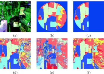
Fig. 4: EstimatedQmatrix for Image 1 (left) and Image 2 (right). Real images – Finally, experiments are conducted on a real600×
600hyperspectral image composed ofD= 349spectral bands (af-ter removing the bands of low SNR) obtained within the MUESLI mission1. First,R = 7endmembers have been extracted by
con-ducting a vertex component analysis [21]. The classification ground-truth provided by the experts after a field campaign is composed of L = 6classes (summer crops, straw cereals, wooded area, build-ings, bare/hayed land, meadow) and the left half of the ground-truth is used as external datacLwith a confidenceηp= 95%(∀p∈ L). 1http://fauvel.mathieu.free.fr/pages/muesli.html
The number of clustersKhas been set to a high value, i.e.,K= 40. The proposed algorithm is expected to empty most of these clusters. Results in term of classification accuracy obtained by the proposed method are compared to those obtained with a state-of-the-art ran-dom forest (RF) classifier, known to be particularly robust to label-ing errors [22]. Parameters of the RF classifier are optimized uslabel-ing
5-folds cross-validation (50trees, maximum depth of20). The quan-titative results are averaged over10trials.
Table 1: Classification results averaged over10trials (±standard deviation).
Cohen’s kappa Time (s) Proposed model 0.737 (±0.030) 6651 (±62) Random forest 0.695 (±0.003) 16 (±0.2)
Experiment results reported in Table 1 show significant better classification results for the proposed model on this particular im-age. Nevertheless, this result is obtained at the cost of more exten-sive computations induced by the MCMC algorithm, as underlined in the same table. However, it is worth noting that the proposed method also provides additional parameters of interest, in terms of abundance and cluster maps. To illustrate, results obtained for a par-ticular trial are displayed in Fig. 5.
(a) (b) (c)
(d) (e) (f)
Fig. 5: Real data: (a) pseudo-colored image, (b) expert ground-truth, (c) training ground-truth, (d) RF classification, (e) obtained cluster-ing and (f) obtained classification (withβ1= 0andβ2= 1.0).
5. CONCLUSION
This paper introduced a new Bayesian model to perform spectral unmixing, clustering and robust classification jointly. Through the clustering step, the two well-admitted hyperspectral analysis meth-ods, namely unmixing and classification, were conducted in a unified framework, benefiting from low-level and high-level descriptions of the data simultaneously. Interestingly, akin to any conventional supervised classification setup, external ground-truth data could be provided. However, the proposed model allowed corrupted ground-truth labels to be taken into account and corrected, resulting in a supervised classification robust to mislabeling. Results conducted on synthetic and real hyperspectral datasets illustrated good perfor-mance in term of classification and underlined the robustness of the model in case of label errors in training data. Future works will focus on the generalization of the proposed model to handle other low-level tasks, i.e., different from spectral unmixing.
6. REFERENCES
[1] J. M. Bioucas-Dias, A. Plaza, N. Dobigeon, M. Parente, Q. Du, P. Gader, and J. Chanussot, “Hyperspectral Unmixing Overview: Geometrical, Statistical, and Sparse Regression-Based Approaches,”IEEE J. Sel. Topics Appl. Earth Observ. in Remote Sens., vol. 5, pp. 354–379, 2012.
[2] A. Plaza, J. A. Benediktsson, J. W. Boardman, J. Brazile, L. Bruzzone, G. Camps-Valls, J. Chanussot, M. Fauvel, P. Gamba, A. Gualtieri, and others, “Recent advances in tech-niques for hyperspectral image processing,”Remote Sens. En-viron., vol. 113, pp. S110–S122, 2009.
[3] N. Dobigeon, S. Moussaoui, M. Coulon, J.-Y. Tourneret, and A. O. Hero, “Joint Bayesian endmember extraction and linear unmixing for hyperspectral imagery,”IEEE Trans. Signal Pro-cess., vol. 57, pp. 4355–4368, 2009.
[4] D. C. Heinz and C. Chang, “Fully constrained least squares linear spectral mixture analysis method for material quantifi-cation in hyperspectral imagery,”IEEE Trans. Geosci. Remote Sens., vol. 39, pp. 529–545, 2001.
[5] G. Camps-Valls, D. Tuia, L. Bruzzone, and J. A. Benediktsson, “Advances in hyperspectral image classification: Earth moni-toring with statistical learning methods,”IEEE Signal Process. Mag., vol. 31, pp. 45–54, 2014.
[6] M. Dalla Mura, A. Villa, J. A. Benediktsson, J. Chanussot, and L. Bruzzone, “Classification of hyperspectral images by us-ing extended morphological attribute profiles and independent component analysis,”IEEE Geosci. Remote Sens. Lett., vol. 8, pp. 542–546, 2011.
[7] M. Fauvel, Y. Tarabalka, J. A. Benediktsson, J. Chanussot, and J. C. Tilton, “Advances in spectral-spatial classification of hy-perspectral images,”Proc. IEEE, vol. 101, pp. 652–675, 2013. [8] A. Villa, J. A. Benediktsson, J. Chanussot, and C. Jutten, “Hyperspectral image classification with independent compo-nent discriminant analysis,”IEEE Trans. Geosci. Remote Sens., vol. 49, pp. 4865–4876, 2011.
[9] A. Villa, J. Li, A. Plaza, and J. M. Bioucas-Dias, “A new semi-supervised algorithm for hyperspectral image classifica-tion based on spectral unmixing concepts,” in Proc. IEEE GRSS Workshop Hyperspectral Image SIgnal Process.: Evo-lution in Remote Sens. (WHISPERS). IEEE, 2011, pp. 1–4. [10] J. Li, I. D´opido, P. Gamba, and A. Plaza, “Complementarity
of discriminative classifiers and spectral unmixing techniques for the interpretation of hyperspectral images,” IEEE Trans. Geosci. Remote Sens., vol. 53, pp. 2899–2912, 2015. [11] O. Eches, J. A. Benediktsson, N. Dobigeon, and J.-Y.
Tourneret, “Adaptive Markov random fields for joint unmix-ing and segmentation of hyperspectral images,” IEEE Trans. Image Process., vol. 22, pp. 5–16, 2013.
[12] P. V. Giampouras, K. E. Themelis, A. A. Rontogiannis, and K. D. Koutroumbas, “Simultaneously sparse and low-rank abundance matrix estimation for hyperspectral image unmix-ing,” IEEE Trans. Geosci. Remote Sens., vol. 54, no. 8, pp. 4775–4789, 2016.
[13] D. F. Nettleton, A. Orriols-Puig, and A. Fornells, “A study of the effect of different types of noise on the precision of su-pervised learning techniques,” Artif. Intell. Rev., vol. 33, pp. 275–306, 2010.
[14] C. Pelletier, S. Valero, J. Inglada, N. Champion, C. Marais Sicre, and G. Dedieu, “Effect of Training Class Label Noise on Classification Performances for Land Cover Mapping with Satellite Image Time Series,” Remote Sens., vol. 9, p. 173, 2017.
[15] C. Bouveyron and S. Girard, “Robust supervised classification with mixture models: Learning from data with uncertain la-bels,”Pattern Recognit., vol. 42, pp. 2649–2658, 2009. [16] S. Z. Li,Markov Random Field Modeling in Image Analysis.
Springer Science & Business Media, 2009.
[17] F.-Y. Wu, “The potts model,”Rev. Mod. Phys., vol. 54, p. 235, 1982.
[18] C. P. Robert and G. Casella,Monte Carlo Statistical Methods, ser. Springer Texts in Statistics. New York, NY: Springer New York, 2004.
[19] A. Lagrange, M. Fauvel, S. May, and N. Dobigeon, “Hierarchical Bayesian image analysis: From low-level modeling to robust supervised learning,” 2017. [Online]. Available: https://arxiv.org/abs/1712.00368
[20] T. Hastie and R. Tibshirani, “Discriminant Analysis by Gaus-sian Mixtures,”J. Roy. Stat. Soc. Ser. B, vol. 58, pp. 155–176, 1996.
[21] J. M. P. Nascimento and J. M. Bioucas-Dias, “Vertex compo-nent analysis: A fast algorithm to unmix hyperspectral data,”
IEEE Trans. Geosci. Remote Sens., vol. 43, pp. 898–910, 2005. [22] A. Folleco, T. M. Khoshgoftaar, J. V. Hulse, and L. Bullard, “Identifying learners robust to low quality data,” inProc. IEEE Int. Conf. on Inf. Reuse and Integr., 2008, pp. 190–195.