Fluid Simulation For Computer Graphics: A Tutorial in Grid Based and Particle
Based Methods
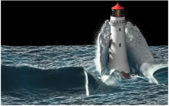
Colin Braley∗ Virginia Tech Adrian Sandu† Virginia TechFigure 1:Fluid Simulation Examples
Abstract
In this paper we present a tutorial on the implementation of both a grid based and a particle based fluid simulator for computer graph-ics applications. Many research papers on fluid simulation are read-ily available, but these papers often assume a very sophisticated mathematical background not held by many undergraduates. Fur-thermore, these papers tend to gloss over the implementation de-tails, which are very important to people trying to implement a working system.
Recently, Robert Bridson release the wonderful book, ”Fluid Simu-lation for Computer Graphics.[Bridson 2009]” We base a large por-tion of our own grid-based simulator off of this text. However, this text is very dense and theory intensive, and this document serves as easy version for those who want to implement a simulator quickly. Furthermore, Bridson’s text does not cover particle based methods, like SPH, which are quickly becoming commonplace within the graphics community. This work provides an introduction to SPH as well.
Keywords: Fluids, Physically Based Animation, SPH, Grid Based
1
Introduction
2
Introduction
In the context of physics, the word fluid may mean something dif-ferent than you might usually think. In physics, fluids fall into two categoriesincompressibleandcompressibleflow. Incompressible flow is a liquid, such as water or juice. Compressible flow, on the other hand, corresponds to gas such as air or steam. Compressible flow is called compressible, because you can easily change the vol-ume of this fluid. Note that there is no such thing as 100 percent incompressible fluid. All fluids, even water can change volume to some degree. If they could not, there would be no way to audi-bly yell under water. However, we simply choose to ignore com-pressibility in fluids like water that are nearly incompressible, and instead we refer to them simply as incompressible.
There are many, many ways to simulate fluids. In graphics, the most common two techniques are grid based simulations, and par-ticle based simulations. (Very recently, new techniques such as the Lattice-Boltzmann method have been introduced to graphics, but they are beyond the scope of this paper.) Grid based simulations
∗e-mail: [email protected] †e-mail:[email protected]
are typically highly accurate, although relatively slow compared to particle based solutions. Particle based simulations are usually much faster, but they typically do not look as good as grid based simulations.
Some readers may not know the difference between grid based and particle based simulations. The best description of this can be found in page 6 of [Bridson 2009]. I will attempt to paraphrase this de-scription here.
Fluid can be simulated from 2 viewpoints,LagrangianorEulerian. In theLagrangianviewpoint, we simulate the fluid as discrete blobs of fluid. Each particle has various properties, such as mass, veloc-ity, etc. The benefit of this approach is that conservation of mass comes easily. TheEulerianviewpoint, on the other hand tracks fixed points inside of the fluid. At each fixed point, we store quan-tities such as the velocity of the fluid as it flows by, or the density of the fluid as it passes by. TheEulerianapproach corresponds to grid based techniques. Grid based techniques have the advantage of hav-ing higher numerical accuracy, since it is easier to work with spatial derivatives on a fixed grid, as opposed to an unstructured cloud of particles. However, grid based techniques often suffer from mass loss, and are often slower than particle based simulations. Finally, grid based simulations often do much better tracking smooth water surfaces, whereas particle based approaches often have issues with these smooth surfaces.
3
Governing Equations
Here we will describe the governing equations for fluid motion, and also describe some of the special notation used in fluid simulation literature. For someone only interested in a basic implementation, this section can be skimmed with the exception of the final para-graph on notation. However, for a full understanding of thewhyin fluid simulation, this section should be read in full.
First, we will describe the general incompressible Navier Stokes equations. We will attempt to intuitively describe the vector cal-culus operators involved, and those without a knowledge of vector calculus may wish to consult the appendix of [Bridson 2009] for review. Here are the incompressible Navier Stokes equations:
∂~u ∂t +~u+ 1 ρ∇p= ~ F+ν∇ · ∇~u (1) ∇ ·~u= 0 (2)
In these equations,~uis fluid velocity. The time variable istThe density of the fluid is represented byρ. For water,ρ ≈1000mkg3. The pressure inside the fluid (in force units per unit area) is repre-sented byp. Note thatpandρare different things(the first is the Greek letterrhowhile the second isp). Body forces (usually just gravity) are represented byF~. Finally,νis the fluid’s coefficient of kinematic viscosity.
In our simulator, we currently don’t take fluid viscosity into ac-count. For inviscid fluids like water, viscosity does usually not play a large role in the look of an animation. However, if you wish to include viscosity, see chapter 8 of [Bridson 2009]. The fundamen-tal work on viscous fluids in graphics is [Goktekin et al. 2004], and can be taken as a starting point for implementation.
When the viscosity term is dropped from the incompressible Navier Stokes equations, we get the following set of equations:
∂~u ∂t + 1 ρ∇p= ~ F (3) ∇ ·~u= 0 (4) These equations are simpler, and they are the equations we will con-sider for the rest of this paper. These are called theEuler Equations. Lastly, we will quickly discuss some unique notation used in fluid simulation. In simulation, we take small discrete time steps in or-der simulate some phenomenon. Consior-der the velocity field~u be-ing simulated. In a grid based simulation, we store~uas a discreetly sampled vector field. However, we need some type of notation to describe which grid element we are referring to. To do this, we use subscripts like the following~ua,b,cto refer to the vector ata, b, c (Note that our indexing scheme is actually more complicated, but this is discussed in the beginning of the grid based simulation sec-tion.) However, we also need a way to indicate which timestep we are referring to. To do this, we use superscripts, such as~uka,b,c. The previous equation would indicate the velocity at indexa, b, c at timestepk. While some would consider this an egregious abuse of notation, this syntax is extremely convenient in fluid simulation. In order to maintain clarity, we will explicitly state when we are raising a quantity to a power (as opposed to indicating a timestep). Furthermore, timesteps are written in bold (ab), whereas exponents are written in a regular script (ab).
4
Grid Based Simulation
4.1 OverviewHere we will present a high level version of the algorithm for grid based fluid simulation, assuming one wants to simulatenframes of animation.
1. Initialize Grid with some Fluid 2. for(ifrom1ton)
Lett= 0.0 Whilet < tf rame
Calculate∆t Advect Fluid
Pressure Projection (Pressure Solve) Advect Free Surface
t=t+ ∆t Write frameito disk
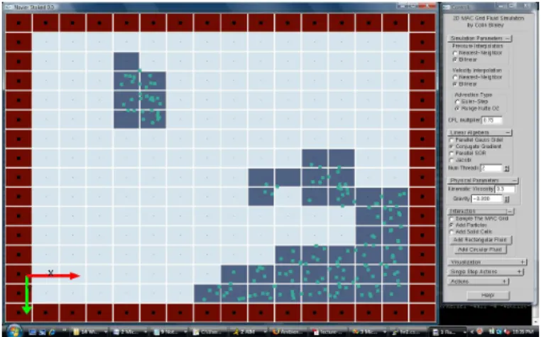
Figure 2:Our 2D Eulerian Solver
4.2 Data Structures
While we have discussed Lagrangian vs. Eulerian viewpoints, we have yet to define what exactly we mean by ”grid” in grid based simulation. Throughout the simulation, we must store many dif-ferent quantities (velocity, pressure, fluid concentration, etc.) at various points in space. Clearly, we will lay them out in some form of regular grid. However, not just any grid will do. It turns out that some grids work much better than others.
Most peoples intuition is to go with the simplest approach: store ev-ery quantity on the same grid. However, for reasons which we will soon discuss, this is not a good approach. Back in the 1950’s the seminal paper [Harlow and Welch 1965a] by Harlow and Welch de-veloped the innovateMAC Gridtechnique. (Note that MAC stands for Marker-and-Cell.) Among many things, this paper developed a new way to track liquid movement through the grid, called marker particles, and a new type of grid, a staggered grid. Marker particles are still used in some simulators for their simplicity, but they are no longer state of the art. However, the staggered grid developed by Harlow and Welch is still used in many, many simulators.
This grid is called staggered because it stores different quantities at different locations. In two dimensions, a single cell in a MAC Grid might look as follows:
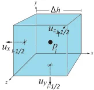
Figure 3:Two Dimensional MAC Cell In three dimensions, a MAC cell would look like this:
Note that in these imagesprepresents pressure, and~uis velocity. We see in these images that pressure is stored in the center of every grid cell, while velocity is stored on the faces of the cells. Note that these velocity samples are the normal component of the velocity at
Figure 4:Three Dimensional MAC Cell
each cell face. We will now describe why the grid is arranged in this manner.
Consider a quantity w sampled at discrete locations w0, w1, . . . wi−1, wi, wi+1, . . . wn−1, wn along the real line. Imagine we want to estimate the derivative at some sample pointi. We must use central differences of some form. Immediately, one can see that:
∂w ∂xi
≈ wi+1−wi−1
2∆x (5)
Recall from numerical analysis that this isO(∆x2)accurate. How-ever, there is clearly a huge problem with this equation. It ignores the actual value ofwatwi! We clearly need a way to estimate this derivative without ignoring the actual value at the point which we are trying to estimate. We could forward or backward differences, but these are biased and onlyO(∆x)accurate. Instead, we choose to stagger our grid to make these accurate central differences work. Our staggered central difference looks like this:
∂w ∂xi≈
wi+1 2 −wi−12
2∆x (6)
This formula is stillO(x2)accurate.
It turns out that, later on in ourPressure Projectionstage, this stag-gered grid is very useful, as it allows us to accurately estimate cer-tain derivatives that we require.
However, this staggered grid is not without drawbacks. In order to evaluate a pressure value at an arbitrary point which is not an exact grid point, trilinear interpolation (or bilinear in the 2D case) is required. If we want to evaluate velocityanywherein the grid, a separate trilinear interpolation is required for each component of the velocity! Therefore, in 3D we need to to 3 trilinear interpolations, and in the 2D case we need to do 2 bilinear interpolations! Clearly, this is slightly unwieldy. However, the added accuracy makes up for the complications in interpolation.
The above notation with half-indices is clearly useful since it greatly simplifies our formulae. However, it is obvious that half-indices can’t be used in an actual implementation. [Bridson 2009] recommends the following formulae for converting these half-indices to array half-indices for a real system:
p[i][j][k] =pi,j,k (7) ux[i][j][k] =ui−1 2,j,k (8) uy[i][j][k] =vi,j−1 2,k (9) uz[i][j][k] =wi,j,k−1 2 (10)
Therefore, for a grid ofnx, ny, nzcells, we store the pressure in a nx, ny, nzarray, the x component of the velocity in anx+1, ny, nz array, the y component of the velocity in anx, ny+ 1, nzarray, and the z component of the velocity in anx, ny, nz+ 1array. 4.3 Algorithm
4.3.1 Choosing a Timestep
When simulating fluids, we want to simulate as fast as possible without losing numerical accuracy. Therefore, we want to chose a timestep that is as large as possible, but not large enough to desta-bilize our simulation. The CFL condition helps us do this. The CFL says to chose a value of∆tsmall enough so that when any quantity is moved from the center of some cell through the velocity field, it will only move∆hdistance. This makes sense intuitively, seeing as if a particle was allowed to move in any larger amounts than this you would effectively be ignoring some parts of the velocity field. Therefore, our equation for∆tis as follows:
∆t= ∆h
~ umax
(11)
As you can see, this requires us to know the maximum velocity in the velocity field at any given time. There are 2 ways to get this value, either by doing a linear search through all of the velocities, or by keeping track of the maximum velocity throughout the sim-ulation. These details are discussed in the Implementation section. In computer graphics, we are often willing to sacrifice strict nu-merical accuracy for the sake of increased computational speed. In many situations, a practitioner is not worried about if the fluid being simulated is one-hundred percent accurate. Instead, we want plau-sible looking results. Therefore, in many applications you can get away with using a timestep larger than that prescribed by the CFL condition. For instance, in [Foster and Fedkiw 2001], the authors were able to use a timestep 5 times bigger than that dictated by the CFL condition. Either way, it is good practice to let the user be able to scale the CFL based timestep by a factor of their choice,kCF L. In this case, our equation becomes:
∆t=kCF L
∆h ~ umax
(12)
f(v, vmax, vmin) =κmin(v−vmin)
κmax−κmin vmax−vmin
(13)
In [Bridson 2009], a slightly more robust treatment of the CFL condition is presented. In this text, Bridson suggests a modification where~umaxis calculated with:
~
umax= max (|~u|) +
q
∆h|F~| (14)
whereF~ is whatever body forces are to be applied (usually just gravity), andmax~uis simply the largest velocity value currently on the grid. This solution is slightly more robust in that it takes into account the effect that the body forces will have on the simulation’s current timestep.
4.3.2 Advection
Central to any grid based method is our ability to advect both scalar and vector quantities through our simulation grid. Advection can be informally described as follows: ”Given some quantityQon our simulation grid, how willQchange∆tlater?” More formally, we can describe advection as:
Qn+1=advect(Qn,∆t,∂Q ∂t
n
) (15)
In this section we will develop a computational function for advect(Qn,∆t,∂Q∂tn).
Consider aPon our simulation grid. Using our central differencing schemes described previously, we can trivially calculate∂Q∂t. Using this derivative, along with our grid information, we can develop a technique to advect quantities through the grid. This technique sometimes called abackwards particle trace. Since we are using a particle, this is also commonly referred to asSemi-Lagrangian Advection. It is important to note that no particle is ever created, and the particle is purely conceptual. This is what leads to theSemi inSemi-Lagrangian Advection.
Note that our algorithm can not be done in place, and requires an extra copy of the pertinent data in our simulation grid. Our algo-rithm works as follows:
1. For each grid cell with indexi, j, k Calculate−∂Q
∂t
Calcluate the spatial position ofQi,j,k, store it inX~ CalculateX~prev=X~ −∂Q∂t ∗∆t
Set the gridpoint forQn+1
that is nearest toX~prevequal toQi,j,k
2. SetQ=Qn+1
This algorithm is very simple, and fairly accurate. However, if you are familiar with numerical analysis, you will recognize that this algorithm uses the simple time integratorForward Euler. This inte-grator is not very accurate. We recommend atleastusing an integra-tor such as RK2 or better (Runge Kutta Order-2). In our simulaintegra-tor, we tested out 5 different integrators, and found the followingO(h3)
accurate scheme to work the best:
κ1=f(Qn) (16) κ2=f(Qn+1 2∆tκ1) (17) κ3=f(Qn+3 4∆tκ2) (18) Qn+1=Qn+2 9∆tκ1+ 3 9∆tκ2+ 4 9∆tκ3 (19)
We will use this advection scheme throughout our simulator. One common use is advecting fluid velocity itself. Another use is ad-vecting temperatures or material properties in advanced simulators. A careful reader might have noticed one issue with the advection psuedocode. How would we perform an advection for a boundary
cell? This requires extrapolation for our MAC grid. In our expe-rience, simply clamping grid indices is fine in the advection code, but more advanced techniques do exist. However, we have found that in practice these advanced extrapolation techniques do little to visually augment the simulation.
4.3.3 Pressure Solve
So far, we have done nothing to deal with the incompressbility of our fluids. In this section, we will develop a numerical routine such that our fluid satisfies both the incompressibility condition:
∇ ·~un+1= 0 (20)
as well as our boundary conditions: ~
un+1·ˆn=~usolid·nˆ (21)
Additionally, this section finally allows us to show the reason for our staggered MAC grid discussed in our previous section. First, we will work out the individual equations to make a single grid cell satisfy our two conditions above. Then, we will show how this information can be used to make the entire grid incompressible. Consider a 2D MAC cell at locationi, j. Per the Euler equations, on every step we must update our cells velocity by the following equations. First, we present them in 2D where our velocity is rep-resented by~u=< u, v >. ~ uni++11 2,j =~uni+1 2,j−∆t 1 ρ pi+1,j−pi,j ∆h (22) ~ vi,jn+1+1 2 =~vi,jn+1 2 −∆t 1 ρ pi,j+1−pi,j ∆h (23)
Here are the equivalent equations in 3D for~u=< u, v, w >.
~ uni++11 2,j,k =~uni+1 2,j,k−∆t 1 ρ pi+1,j,k−pi,j,k ∆h (24) ~vi,jn+1+1 2,k =~vi,jn+1 2,k−∆t 1 ρ pi,j+1,k−pi,j,k ∆h (25) ~ wi,j,kn+1+1 2 =w~ni,j,k+1 2 −∆t 1 ρ pi,j,k+1−pi,j,k ∆h (26)
Just in case these don’t seem complicated enough already, there is another issue that must be attended to. These equations are only ap-plied tocomponentsof the velocity that border a grid cell that con-tain fluid. Getting these conditions correct was one of the hardest things in the actual programming of our simulation, and we recom-mend that an implementor try to first program this in 2D for easier debugging.
A careful reader will also notice that these equations may require the pressures of grid cells that lie either outside of the grid, or out-side of the fluid. Therefore, we must specify our boundary condi-tions.
There are two primary types of boundary conditions in grid based simulation,DirichletandNeumann. We will use Dirichlet condi-tions for free surface boundaries, indicating that we will specify the value of the quantity at and boundary case. Therefore, we simply assume that pressure is0in any region of air outside of the fluid.
The more complicated boundary is with solid walls. Here we will use aNeumannboundary condition. Using the above pressure up-date equations, we substitute in the solids velocity (0 for simula-tions without moving solids), and then we arrive at a single linear equation for our pressure. Rearranging our terms allows us to solve for the pressure.
Now we will work out how to make our fluid incompressible. This means that, for every velocity component on the grid, we want to satisfy:
∇ ·~u= 0 (27) Note that this divergence operator can be expanded to:
∇ ·~u= ∂u ∂x+ ∂v ∂y+ ∂w ∂z (28)
Therefore, it is clear that we simply want to find a way so that each component of our spatial derivatives equals zero. Recalling our cen-tral differences used earlier, we can approximate these divergences using the following numerical routines, which use our finite differ-ences developer earlier:
(∇·~u)i,j,k≈ ~ ui+1 2,j,k−~ui− 1 2,j,k ∆h + ~ vi,j+1 2,k−~vi,j− 1 2,k ∆h + ~ wi,j,k+1 2 −w~i,j,k− 1 2 ∆h (29) Finally, we have all the quantities necessary for our pressure update. We have developed equations for how the pressure affects the veloc-ity, and we also have numerical equations to estimate the pressure gradient. Using this information, we can create a linear equation for the new pressure in every grid cell. We can then combine these equations together into a system of simultaneous linear equations which we can solve for the whole grid, and finally complete our pressure update.
Eventually, we hope to end up with a system of equations of the form:
A~x=~b (30)
Every row ofAcorresponds to one equation for one fluid cell. In this formulation, we will setup our matrix such that~bis simply our negative divergences for every fluid cell. When written out, our linear system takes the following form:
−Ω1 β1,2 . . . β1,n β2,1 −Ω2 ... .. . −. .. βn−1,n βn,1 . . . βn,n−1 −Ωn p1 p2 .. . pn−1 pn = −D1 −D2 .. . −Dn−1 −Dn (31) In this equation,Diis the divergence through celli,Ωiis the num-ber of non-solid neighbors of celli, andβijtakes values based on the below equation:
βij=
(
1 if celliis a neighbor of cellj
0 otherwise. (32)
Our matrixAhas many unique properties we can exploit both in our choice of linear solver and in our storage ofAitself. It is immedi-ately clear thatAis sparse(most of its entires are zero), indicating
we should store is as asparse matrix. Each row has at most 4 non-zero entries in the 2D case, and 6 non-non-zero entries in the 3D case. Furthermore, is is clear thatAis symmetric. Every entry at index i, jthat is not on the main diagonal is defined byβi,j. Through our definition ofβ, it is clear thatβi,j =βj,i. Therefore, we only need to store half of the entries inA. We use the following scheme for storing our matrix. We store a main linked list, sorted first by column, then by row. We store in each linked list node the following < i, j, pij >. The column index is stored asi, the row index is stored byj, and the corresponding pressure value is stored as p. This storage scheme has many pros and cons. We are storing the minimum amount of data, as we are storing only half of the matrix’s non-zero entries. However, this memory saving comes at the cost of speed. Accessing an arbitrary matrix entry isO(1
2n) = O(n), which can be slow. For small simulations where memory usage is not a concern, we recommend including the option to store entries in a dense matrix.
Finally, a reader highly experienced in numerical analysis will real-ize thatAhas a form that is common to many other matrices. In 2D, Ais often called the5 point Laplacian Matrix, whereas in 3D it is called the7 Point Laplacian Matrix. Bridson recommends the Mod-ified Incomplete Cholesky Conjugate Gradient Level 0algorithm [Bridson 2009]. Essentially, this is simply the conjugate gradient algorithm with a special preconditioner designed for this particular matrix. If the reader is interested in implementing their own con-jugate gradient solver, we recommend the paper [Shewchuk 2007] as a good starting point. However, in our implementation we are not planning on dealing with enormous bodies of water so we im-plemented both the regularConjugate Gradientalgorithm, as well asParallel Successive Over-Relaxation(Parallel SOR), and the Ja-cobi Method. We found the parallel SOR to be faster than the con-jugate gradient implementation, but this is probably because we are not using a preconditioner. However, conjugate gradient was slightly faster than the Jacobi method in our tests. Note that we used OpenMP for parallelizing our SOR implementation. We hope to add a preconditioner to our conjugate gradient implementation in the near future.
While we have described the characteristics of the linear system to solve, and what kind of solvers to use, we realize that most readers will not want to spend their time writing a highly optimized im-plementation of a specialized conjugate gradient solver. Therefore, we will quickly direct the reader towards a few good linear algebra packages that have routines that suit our purposes:
• BoostµBLAS
• SparseKit
• http://people.cs.ubc.ca/ rbridson/mpcg/ Open Source Matlab Implementation of Specialized Form of Conjugate Gradient
4.3.4 Grid Update
4.4 Tracking the Water Surface In Grid Bases Simula-tion
While we have discussed the basic mechanisms for a grid based simulation, we have not discussed how to unify all these ideas into a full working simulator that can output data that encapsulates the position of a moving water surface.
There are many ways to approach the problem of tracking the move-ment of water through a simulation grid. The simplest way, in-troduced all the way back in Harlow and Welch’s seminal paper [Harlow and Welch 1965b]. This approach is relatively simple, and still quite useful. Here we store a collection of many discrete
marker particlesin our simulation, each representing a water parti-cle. Every timestep, we advect them through the velocity field by
∆t. Also, we store an enumeration value inside of each cell indi-cating whether the cell contains liquid, air, or solid. Once a fluid marker particle moves into a cell, we mark it as liquid. This is nec-essary for our pressure solve. After each timestep, we can output these particles to disk. However, the question remains as to how to render these particles. One approach is to use a implicit surface function to generate a water surface from these particles. We dis-cuss this approach later, in section the section on surfacing SPH simulations. Unfortunately, this approach can lead to blobby, ugly surfaces. Therefore, we turn to alevel-setbased approach, first in-troduced in [?].
Level set methods are currently the best way to achieve smooth high quality free surfaces in liquid simulation. However, they are far more computationally expensive than the above implicit surface approach. Here we will present a brief introduction to these tech-niques. We recommend that an interested reader refer to [Fedkiw and Sethian 2002] for more detailed information.
For the level set method, we define a new value,φi,j,k, at the center of all of our simulation cells. We define our liquid free surface to exist at locations where the following equation is satisfied:
φ(X~) = 0 (33)
WhereX~ is a position vector. Note that we can defineΦ(X~)at non-grid cell locations through any type of interpolation, either trilinear or Catmull-Romm is a fine choice.
Furthermore, we say that locations that satisfyφ(X~) < 0to be inside of the water, andφ(X~) <0to be outside of the water. To representφ, we use a function called thesigned distance function. Given an arbitrary setSofkSkpoints, we define our signed dis-tance functionD(X~)as:
DS(X~) =min~p∈SkX~−~pk (34) Clearly, for some arbitrary pointX~, the magnitude of the signed distance is the distance to the nearest point in the setS. Signed distance is also useful because of another property. If we want to check whether a grid cell is inside or outside of the fluid, all we must do is examine the sign of the signed distance.
Thus far we have ignored an important problem with signed dis-tance: how to compute it. At the beginning of a simulation, we can assume our signed distance function is already computed on the grid.
There are many ways to calculate signed distance, and new problem-specific techniques are developed frequently. Typically, people classify these methods into two groups: PDE based ap-proaches and Geometric Approaches. PDE Based techniques approximate something called the Eikonal Equation, k∇φk = 1. These techniques are mathematically and computationally in-volved, and are often overkill for graphics work. Instead, we will discuss briefly the geometric approaches. Our discussion will not go into much depth; for a more in depth treatment of geometric algorithms for computing signed distance see [?].
Our algorithms for computing signed distance take the following general form:
1. Set the signed distance of each grid-point to ”unknown”
2. for each grid pointPdirectly at the free-surface, set the signed distance to0
3. Loop over each grid-pointGi,j,kat which signed distance is unknown
Loop over each grid-pointP that neighbors Gi,j,k as long as the signed distance atP is known
Find the distance fromGi,j,k to the surface points. If this distance is closer thanP’s signed distance, markP as unknown once again
Take the minimum value of the distances of the neigh-bors, and determine ifGi,j,kis inside or outside, and set the sign of the distance based on this
There are two main techniques for implementing such an algorithm. These techniques are thefast marching method, and thefast sweep-ing method.
The fast marching method loops over the closest grid points first, and then those that are farther away. This technique works rapidly by storing the unknown grid points in apriority queuedata struc-ture. This algorithm runs inO(nlog(n))when the priority queue is implemented with a heap. A detailed description can be found in [Sethian 1999].
The other technique is the fast sweeping method. The fast sweeping method takes the opposite approach from the fast marching method. Here, we allow the signed distance function to first be calculated at our farthest away points. We then have this information propagate back towards the surface. Fast marching is great because it isO(n), and is very simple. Furthermore, it works well withnarrow band methods, discussed in [Bridson 2009] and [Fedkiw et al. 2001a]. While we have discussed how to compute a signed distance func-tion, we have not discussed how to update the signed distance as the fluid’s free surface moves. While this may seem complicated, this step is quite trivial. Since ourφvalues are stored in the cen-ter of our grid cells, we can simply advect these values according to the fluid’s velocity. However, it turns out that advection does not perfectly preserve signed distance. Therefore, we periodically recalculate our signed distance every few timesteps. Bridson rec-comends that we recalculate our signed distance once per frame (note that typically many timesteps of∆tare required per frame) [Bridson 2009].
TODO: Finish this section. I am still working on it since my level set implementation is not complete.
5
Particle Based Simulation
5.1 OverviewIn this section we describe an alternative approach to fluid simula-tion. Here we discussLagrangiantechniques. In this approach, we have a set of discrete particles that move through space to represent our fluid. We no longer simulate our fluid on a grid structure. This approach has many pros and cons compared to grid based tech-niques. In general, particle based approaches are less accurate than their grid based counterparts. This is primarily due to the difficul-ties in dealing with spatial derivatives on an unstructured particle cloud. However, particle based simulations are typically much eas-ier to program and understand. Furthermore, particle based tech-niques are much faster, and can be used in real time applications such as video games.
We will describe Smoothed Particle Hydrodynamics. This tech-nique was originally introduced for astrophysical simulations[?], but has also found a lot of uses in computer graphics [?]. This description is especially valuable, since SPH is not discussed in Bridson’s text[Bridson 2009], and crucial implementation details are scattered through both astophyics, computational fluid dynam-ics, and computer graphics literature.
Figure 5:Our Simple 2D SPH Implementation
5.2 Data Structures
First, we must outline what information we need to store for our simulation. Clearly, we need a data structure to list all of our parti-cles. Since particles must frequently be added to the simulation, we will choose a linked list. However, the question remains as to what information is stored in each particle.
Clearly, we need to store position, velocity, mass, density, and pres-sure. It turns out to be useful to store color and a force vector as well, so we will store these. We will refer to these quantities with the following variables throughout our discussion:
• X~ Position
• V~ Velocity
• MMass
• dDensity
• ρPressure
• C~ =< Cred, Cgreen, Cblue>Color
• F~Force
Note that for our color, each component of the color is∈ [0,1]. Each particle can be trivially implemented as a C structure. Nota-tionally, we will refer to particles with the variableP, and individ-ual particles using subscript notation. For instance, thei-th particle would bePi. Finally, we will refer to particle quantities in a similar manner. For example, the mass of the12th
particle would beM12. 5.3 Algorithm
Our final goal is to satisfy the following condition: For all particlesPi:
∂ ~V ∂ti
=A~pressurei +A~viscosityi +A~gravityi +A~externali (35)
Note that in this equation,A~somethingi refers to the acceleration on particleidue to ”something.” Also, recall from basic physics (F =M
A) thatAi= Fi Mi.
In order for our simulation to progress, we need a way to calculate fluid density at some arbitrary point.
Certain particle properties, such as mass, are given initial values at the beginning of the simulation and are not expected to change. However, other properties must be recalculated every step. Con-sider the pressure property. Here is how to determine the new pres-sure every time step:
However, we have a discrete cloud off particles, so we must use a discrete summation to approximate this integral. This leads us to the equation:
n
X
j6=i
MjWRij (36)
Here,Rijis equal to the Euclidean distance between particleiand particlej.
This functionW(d)is known as akernel function. This function takes a single scalar parameter, which is a distance between two particles, and returns a scalar∈ [0,1]. Typically, a kernel func-tion maps particles that are farther away to values closer to0. This makes sense, since particles far away will not have a large influence on a particle.
Once particles are far enough away from the source, the kernel function drops to0, and therefore these particles no longer have to be considered. We will exploit this fact in a later section when developing acceleration structures for SPH simulations.
The question of what kernel function is best is still a very open research question. However, since our simulations are targeted at begin visually pleasing, rather than scientifically accurate, we do not care much about this. The following kernel function has been used extensively in research and practical applications. This is the Gaussian Kernel. W(d) = 1 π32h3 exp(r 2 h2) (37)
Hereris a the distance between two particles,his our smoothing width. Once particles are greater than distance2haway, they will no longer affect the particles in question. Clearly, larger values of hwill make for a more realistic simulation, albeit at the expense of computational speed.
Finally, we present full psueo-code for an SPH simulation:
• Initialize all particles
• Sett= 0
• Choose a∆t
• forifrom0ton
forjfrom1tonumparticles Get listLjof neighbors forPj CalculateDensityjforPjusingLj CalculateP ressurejforPjusingLj
Calculate accelerationAjforPjusingDensityjand P ressurej
MovePjusingAjand∆tusing Euler step t=t+ ∆t
• Cleanup all data structures
• Exit
5.4 Acceleration Structures
As described above, there is a clear computational bottleneck in our application. We must calculate interaction forces between each and every particle. This is anO(n2)process, which is not computa-tionally viable. By using spatial data structures, we can reduce our computation time toO(n)in the typical case. In the worst case, where all of the particles are in one cell, our algorithm still runs O(n2)Advanced techniques using quadtrees in 2D, or octrees in 3D, can eliminate this possibility.
In addition to storing all of our particles in a linked list, we also store them in a spatial grid data structure. Our grid cells extend by a distance ofRin each dimension. Therefore, in order to cal-culate the forces on a particular particle, one must only examine
9grid cells in the 2D case, or27grid cells in the 3D case. This is because, for any grid cells far enough away, our kernel function will evaluate to0and their contributions will not be included on the current particle. In our experience, including this spatial grid can decrease simulation time by over an order of magnitude for large enough simulations.
However, the addition of this grid data structure requires additional book-keeping during the simulation process. Whenever a particle is moved, one must remove it from its current grid cell, and add it to the grid cell it belongs in. Unfortunately, there is no way to do this simulation in place, and one must maintain two copies of the simulation grid.
Additionally, this fixed grid requires us to change our kernel tion. Oftentimes, implementors in graphics define their kernel func-tions using a piecewise function. If the particles are less than some distancehapart, they evaluate some type of spline. If the particles are farther away, the kernel instead evalutes to0. However, more advanced kernels exist for these types of simulations, and they have recently been used with success in graphics. One of the most com-mon advanced kernels is the cubic spline kernel.
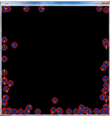
Figure 6:Our 2D SPH Implementation with Lookup Grid Finally, SPH can be further optimized in another way. SPH is clearly very data parallel. Therefore, each particle can be simu-lated in a separate thread with relative ease. Because of this, many high performance SPH implementations are done on the GPU.
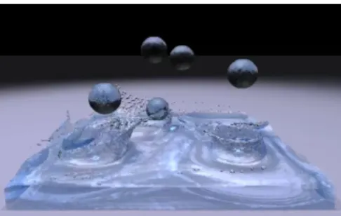
Figure 7:Raytraced GPU Based 3D SPH from University of Tokyo
5.5 Surface Tracking
At our current stage, all SPH results in is an unorganized point cloud of fluid particles. This is unacceptable for most applications. Usually the compuiter graphics practitioner desires a way to render these fluids using a off-the-shelf 3D renderer. In this section, we will outline a few techniques for transforming the result of our SPH simulations into a renderable form.
T and probably the easiest technique, is to sample our SPH results onto a uniform grid. Here we can step through the uniform grid points, and sample the fluid density on these points. Then, we can use this uniform grid as input to an application that performs iso-surface volume rendering. Here we have a choice betweendirect volume rendering, such as that presented in [Colin Braley 2009], andmarching cubes[Lorenson and Cline 1982]. Direct volume ren-dering, typically done through volume raycasting, has the advan-tage of speed. However, there is no easy way to integrate this result-ing image with other generated images, and therefore this technique is only suitable for creating previews. Marching cubes, on the other hand, produces triangle meshes. These meshes are suitable for use in a 3D animation program, and this is therefore a viable option for final production.
While there are benefits to sampling our SPH onto a grid, there are other techniques that often produce better results. Usually, these techniques use a special function for each particle that, whe com-bined with the other particles, produces a fluid surface.
The function usually used for this purpose was introduced by [Blinn 1982]. This technique is often referred to asmeta-ballsorblobbies in the graphics community.
F(X~) = Σnik(
kX~−x~ik
h ) (38)
Whereh is a user specified parameter representing the smooth-ness of the surface, andkis a kernel function like the one repre-sented above. Incremenetal improvements have been made to the the above function throughout the years, the most imporortant of which is presetned in [Williams 2008].
5.6 Extensions
This document has only scratched the surface in discussing the cur-rent state of the art fluid simulation techniques. For a thorough explanation of grid based methods, see [Bridson 2009]. No com-parable resource for SPH and particle based technique exists, but the author recommends reading the papers of Nils Theurey, and the SIGGRAPH 2006 Fluid Simulation Course Notes as a starting point.
Other active areas of fluid simulation research in the graphics com-munity include, smoke simulation, fire simulation, simulation of highly viscous fluids, and coupled simulations. Coupled simula-tions combine two or more simulasimula-tions and get them to interact plausibly. Recently, Ron Fedkiw’s group achieved 2-way coupled SPH and grid based simulations in [?]. Furthermore, examples of couplings with thin shells, rigid body simulations, soft body simu-lations, and cloth simulations exist as well.
Figure 9: Two Way Coupled SPH and Grid Based Simulation by Ron Fedkiw’s Group
Acknowledgments
Thanks to Robert Hagan for editing this work.
References
BATTY, C.,ANDBRIDSON, R. 2008. Accurate viscous free sur-faces for buckling, coiling, and rotating liquids. InProceedings of the 2008 ACM/Eurographics Symposium on Computer Ani-mation, 219–228.
BATTY, C., BERTAILS, F.,ANDBRIDSON, R. 2007. A fast varia-tional framework for accurate solid-fluid coupling. ACM Trans. Graph. 26, 3, 100.
BLINN, J. F. 1982. A generalization of algebraic surface drawing. ACM Trans. Graph. 1, 3, 235–256.
BRIDSON, R. 2009. Fluid Simulation For Computer Graphics. A.K Peters.
COLINBRALEY, ROBERTHAGAN, Y. C. D. G. 2009. Gpu based isosurface volume rendering using depth based coherence. Sig-graph Asia Technical Sketches.
FEDKIW, R.,ANDSETHIAN, J. 2002. Level Set Methods for Dy-namic and Implicit Surfaces.
FEDKIW, R., STAM, J.,ANDJENSEN, H. W. 2001. Visual sim-ulation of smoke. InProceedings of SIGGRAPH 2001, ACM Press / ACM SIGGRAPH, E. Fiume, Ed., Computer Graphics Proceedings, Annual Conference Series, ACM, 15–22.
FEDKIW, R., STAM, J.,ANDJENSEN, H. W., 2001. Visual simu-lation of smoke.
FOSTER, N.,ANDFEDKIW, R. 2001. Practical animation of liq-uids. InSIGGRAPH ’01: Proceedings of the 28th annual con-ference on Computer graphics and interactive techniques, ACM Press, New York, NY, USA, 23–30.
GOKTEKIN, T. G., BARGTEIL, A. W.,ANDO’BRIEN, J. F. 2004. A method for animating viscoelastic fluids. ACM Transactions on Graphics (Proc. of ACM SIGGRAPH 2004) 23, 3, 463–468. GUENDELMAN, E., SELLE, A., LOSASSO, F.,ANDFEDKIW, R.
2005. Coupling water and smoke to thin deformable and rigid shells. In SIGGRAPH ’05: ACM SIGGRAPH 2005 Papers, ACM, New York, NY, USA, 973–981.
HARLOW, F., ANDWELCH, J., 1965. Numerical calculation of time-dependent viscous incompressible flow of fluid with a free surface. the physics of fluids 8.
HARLOW, F., ANDWELCH, J., 1965. Numerical calculation of time-dependent viscous incompressible flow of fluid with a free surface. the physics of fluids 8.
HARLOW, F., ANDWELCH, J., 1965. Numerical calculation of time-dependent viscous incompressible flow of fluid with a free surface. the physics of fluids 8.
LORENSON, ANDCLINE. 1982. Marching cubes. ACM Trans. Graph. 1, 3, 235–256.
PETER, M. C., MUCHA, P. J., BROOKS, R., III, V. H., AND
TURK, G., 2002. Melting and flowing.
PETER, M. C., MUCHA, P. J.,ANDTURK, G. 2004. Rigid fluid: Animating the interplay between rigid bodies and fluid. InACM Trans. Graph, 377–384.
SETHIAN, J. A. 1999.Level Set Methods and Fast Marching Meth-ods: Evolving Interfaces in Computational Geometry, Fluid Me-chanics, Computer Vision, and Materials Science (Cambridge ... on Applied and Computational Mathematics), 2 ed. Cambridge University Press, June.
SHEWCHUK, J. R. 2007. Conjugate gradient without the agonizing pain. Tech. rep., Carnegie Mellon.
STAM, J. 1999. Stable fluids. 121–128.
WILLIAMS, B. W. 2008. Fluid Surface Reconstruction from Par-ticles. Master’s thesis, University of British Columbia.