Technical Report
Number 650
Computer Laboratory
UCAM-CL-TR-650
ISSN 1476-2986
Parallel iterative solution method for
large sparse linear equation systems
Rashid Mehmood, Jon Crowcroft
October 2005
15 JJ Thomson Avenue
Cambridge CB3 0FD
United Kingdom
c
2005 Rashid Mehmood, Jon Crowcroft
Technical reports published by the University of Cambridge
Computer Laboratory are freely available via the Internet:
Parallel iterative solution method for large sparse linear
equation systems
Rashid Mehmood and Jon Crowcroft
University of Cambridge Computer Laboratory, Cambridge, UK.
Email:
{
rashid.mehmood, jon.crowcroft
}
@cl.cam.ac.uk
Abstract
Solving sparse systems of linear equations is at the heart of scientific computing. Large sparse systems often arise in science and engineering problems. One such problem we consider in this paper is the steady-state analysis of Continuous Time Markov Chains (CTMCs). CTMCs are a widely used formalism for the performance analysis of computer and communi-cation systems. A large variety of useful performance measures can be derived from a CTMC via the compu-tation of its steady-state probabilities. A CTMC may be represented by a set of states and a transition rate matrix containing state transition rates as coefficients, and can be analysed using probabilistic model check-ing. However, CTMC models for realistic systems are very large. We address this largeness problem in this paper, by considering parallelisation of symbolic meth-ods. In particular, we consider Multi-Terminal Bi-nary Decision Diagrams (MTBDDs) to store CTMCs, and, using Jacobi iterative method, present a parallel method for the CTMC steady-state solution. Employ-ing a 24-node processor bank, we report results of the sparse systems with over a billion equations and eigh-teen billion nonzeros.
1 Motivation
Solving systems of linear equations is at the heart of scientific computing. Many problems in science and engineering give rise to linear equation systems, such as, forecasting, estimation, approximating non-linear problems in numerical analysis and integer factorisa-tion: another example is the steady-state analysis of
Continuous Time Markov Chains (CTMCs), a prob-lem which we will focus on in this document.
Discrete-state models are widely employed for mod-elling and analysis of communication networks and computer systems. It is often convenient to model such systems as continuous time Markov chains, provided probability distributions are assumed to be exponen-tial. A CTMC may be represented by a set of states and a transition rate matrix containing state transition rates as coefficients, and can be analysed using
proba-bilistic model checking. Such an analysis proceeds by specifying desired performance properties as some tem-poral logic formulae, and by automatically verifying these properties using the appropriate model checking algorithms. A core component of these algorithms is the computation of thesteady-state probabilitiesof the CTMC. This is reducible to the classical problem of solving a sparse system of linear equations, of the form
Ax = b, of size equal to the number of states in the CTMC.
A limitation of the Markovian modelling approach is that the CTMC models tend to grow extremely large due to the state space explosion problem. This is caused by the fact that a system is usually composed of a number of concurrent sub-systems, and that the size of the state space of the overall system is generally exponential in the number of sub-systems. Hence, real-istic systems can give rise to much larger state spaces, typically over 106. As a consequence, much research
is focused on the development of techniques, that is, methods and data structures, which minimise the com-putational (space and time) requirements for analysing large and complex systems.
A standard approach for steady-state solution of CTMCs is to useexplicit methods– the methods which store the state space and associated data structures us-ing sparse storage techniques inherited from the linear algebra community. Standard numerical algorithms can thus be used for CTMC analysis. These explicit approaches typically provide faster solutions due to the fast, array-based data structures used. However, these can only solve models which can be accommodated by the RAM available in contemporary workstations. The so-called (explicit)out-of-coreapproaches [16, 39] have used disk memory to overcome the RAM limita-tions of a single workstation, and have made significant progress in extending the size of the solvable models on a single workstation. A survey of the out-of-core solu-tions can be found in [45].
Another approach for CTMC analysis comprises im-plicit methods. The so-called implicit methods can be traced back toBinary Decision Diagrams (BDDs) [6] and the Kronecker approach [56]. These rely on
ex-ploiting the regularity and structure in models, and hence provide an implicit, usually compact, represen-tation for large models. Among these implicit tech-niques, the methods which are based on binary deci-sion diagrams and extendeci-sions thereof are usually known as symbolic methods. Further details on Kronecker-based approaches and symbolic methods can be found in the surveys, [9] and [53], respectively. A limitation of the pure implicit approach is that it requires ex-plicit storage of the solution vector(s). Consequently, the implicit methods have been combined with out-of-core techniques to address the vector storage limita-tions [40]. A detailed discussion and analysis of both the implicit and explicit out-of-core approaches can be found in [49].
Shared memory multiprocessors, distributed mem-ory computers, workstation clusters and Grids provide a natural way of dealing with the memory and com-puting power problems. The task can be effectively partitioned and distributed to a number of parallel processing elements with shared or distributed mem-ories. Much work is available on parallel numerical iterative solution of general systems of linear equa-tions, see [4, 19, 58], for instance. Parallel solutions for Markov chains have also been considered: for explicit methods which have only used the primary memories of parallel computers, see e.g. [44, 1, 51, 10]; and, for a combination of explicit parallel and out-of-core solu-tions; see [37,36,5]. Parallelisation techniques have also been applied to the implicit methods. These include the Kronecker-based parallel approaches [8,21,35]; and the parallel approaches [43, 64], which are based on a modified form [49] ofMulti-Terminal Binary Decision Diagrams (MTBDDs). MTBDDs [14, 3] are a simple extension of binary decision diagrams; these will be discussed in a later section of this paper.
In this paper, we consider parallelisation of the sym-bolic methods for the steady-state solution of CTMCs. In particular, for our parallel solution, we use the mod-ified form of MTBDDs which was introduced in [49,47]. We chose this modified MTBDD because it provides an extremely compact representation for CTMCs while delivering solution speeds almost as fast as the sparse methods. Secondly, because (although it is symbolic) it exhibits a high degree of parallelism, it is highly con-figurable, and allows effective decomposition and ma-nipulation of the symbolic storage for CTMC matrices. Third, because the time, memory, and decomposition properties for these MTBDDs have already been stud-ied for very large models, with over a billion states; see [49].
The earlier work ( [43,64]) on parallelising MTBDDs have focused on keeping the whole matrix (as a single MTBDD) on each computational node. We address the limitations of the earlier work by presenting a allel solution method which is able to effectively
par-tition, distribute, and manipulate the MTBDD-based symbolic storage. Our method, therefore, is scalable to address larger models.
We present a parallel implementation of the MTBDD-based steady-state solution of CTMCs using the Jacobi iterative method, and report solutions of models with over 1.2 billion states and 16 billion tran-sitions (off-diagonal nonzeros in the matrix) on a pro-cessor bank. The propro-cessor bank which simply is a collection of loosely coupled machines, consists of 24 dual-processor nodes. Using three widely used CTMC benchmark models, we give a fairly detailed analysis of the implementation of our parallel algorithm employ-ing up to 48 processors. Note that the experiments are performed without an exclusive access to the processor bank.
The rest of the paper is organised as follows. In Section 2, we give the background material which is related to this paper. In Section 3, we present and dis-cuss a serial block Jacobi algorithm. In Section 4, in the context of our method we discuss some of the main issues in parallel computing, and describe our paral-lel algorithm and its implementation. The experimen-tal results from the implementation, and its analysis is given in Section 5. In Section 6, the contribution of our work is discussed in relation to the other work on parallel CTMC solutions in the literature. Section 6 also gives a classification of the parallel solution ap-proaches. Section 7 concludes and summarises future work.
2 Background Material
This section gives the background material. In Sec-tions 2.1 to 2.4, and Section 2.6, we briefly discuss it-erative solution methods for linear equation systems. In Section 2.5, we explain how the problem of com-puting steady-state probabilities for CTMCs is related to the solution of linear equation systems. Section 2.7 reviews the relevant sparse storage schemes. We have used MTBDDs to store CTMCs; Section 2.8 gives a short description of the data structure. Finally, in Sec-tion 2.9, we briefly introduce the case studies which we have used in this paper to benchmark our solution method. Here, using these case studies, we also give a comparison of the storage requirements for the main storage schemes.
2.1 Solving Systems of Linear Equations
Large sparse systems of linear equations of the form
Ax=boften arise in science and engineering problems. An example is the mathematical modelling of physical systems, such as climate modelling, over discretized do-mains. The numerical solution methods for linear sys-tems of equations, Ax=b, are broadly classified into two categories: direct methods, such asGaussian
elim-ination, LU factorisation etc; and iterative methods. Direct methods obtain the exact solution in finitely many operations and are often preferred to iterative methods in real applications because of their robust-ness and predictable behaviour. However, as the size of the systems to be solved increases, they often become almost impractical due to the phenomenon known as
fill-in. The fill-in of a sparse matrix is a result of those entries which change from an initial value of zero to a nonzero value during the factorisation phase, e.g. when a row of a sparse matrix is subtracted from another row, some of the zero entries in the latter row may be-come nonzero. Such modifications to the matrix mean that the data structure employed to store the sparse matrix must be updated during the execution of the algorithm.
Iterative methods, on the other hand, do not mod-ify matrix A; rather, they involve the matrix only in the context of matrix-vector product (MVP) opera-tions. The term “iterative methods” refers to a wide range of techniques that use successive approximations to obtain more accurate solutions to a linear system at each step [4]. Beginning with a given approximate solution, these methods modify the components of the approximation, until convergence is achieved. They do not guarantee a solution for all systems of equations. However, when they do yield a solution, they are usu-ally less expensive than direct methods. They can be further classified into stationary methods like Jacobi
and Gauss-Seidel (GS), and non-stationary methods such as Conjugate Gradient, Lanczos, etc. The vol-ume of literature available on iterative methods is huge, see [4,2,24,25,58,38]. In [59], Saad and Vorst present a survey of the iterative methods; [61] describes iterative methods in the context of solving Markov chains. A fine discussion of the parallelisation issues for iterative methods can be found in [58, 4].
2.2 Jacobi and JOR Methods
Jacobi method belongs to the category of so-called sta-tionary iterative methods. These methods can be ex-pressed in the simple form x(k)=F x(k−1)+c, where
x(k)is the approximation to the solution vector at the
k-th iteration and neither F norcdepend onk. To solve a system Ax = b, where A ∈ Rn×n, and
x, b ∈ Rn, the Jacobi method performs the following
computations in itsk-th iteration:
x(ik)=a−ii1(bi − X j6=i aijx (k−1) j ), (1)
for alli, 0≤i < n. In the equation,aijdenotes the
el-ement in rowiand columnjof matrixAand,x(ik)and
x(ik−1)indicate thei-th element of the iteration vector for the iterations numbered kand k−1, respectively. The Jacobi equation given above can also be written
in matrix notation as:
x(k)=D−1(L+U)x(k−1) + D−1b, (2)
where A = D − (L + U) is a partitioning of A
into its diagonal, lower-triangular and upper-triangular parts, respectively. Note the similarities between
x(k) = F x(k−1) + c and Equation (2).
The Jacobi method does not converge for all linear equation systems. In such cases, Jacobi may be made to converge by introducing anunder-relaxation param-eter in the standard Jacobi. Furthermore, it may also be possible to accelerate the convergence of the stan-dard Jacobi method by using anover-relaxation param-eter. The resulting method is known asJacobi overre-laxation(JOR) method. A JOR iteration is given by
x(ik)=αxˆi(k)+ (1−α)x(ik−1), (3)
for 0 ≤ i < n, where ˆxdenotes a Jacobi iteration as given by Equation (1), andα∈(0,2) is the relaxation parameter. The method is under-relaxed for 0< α <
1, and is over-relaxed for α > 1; the choice α = 1 reduces JOR to Jacobi.
Note in Equations (1) and (3), that the order in which the equations are updated is irrelevant, since the Jacobi and the JOR methods treat them indepen-dently. It can also be seen in the Jacobi and the JOR equations that the new approximation of the iteration vector (x(k)) is calculated using only the old approxi-mation of the vector (x(k−1)). These methods, there-fore, possess high degree of natural parallelism. How-ever, Jacobi and JOR methods exhibit relatively slow convergence.
2.3 Gauss-Seidel and SOR
The Gauss-Seidel method typically converges faster than the Jacobi method by using the most recently available approximations of the elements of the itera-tion vector. The other advantage of the Gauss-Seidel algorithm is that it can be implemented using only one iteration vector, which is important for large linear equation systems where storage of a single iteration vector alone may require 10GB or more. However, a consequence of using the most recently available so-lution approximation is that the method is inherently sequential – it does not possess natural parallelism (for further discussion, see Section 4, Note 4.1). The Gauss-Seidel method has been used for parallel solutions of Markov chains, see [43, 64].
The successive over-relaxation (SOR) method ex-tends the Gauss-Seidel method using a relaxation fac-torω∈(0,2), analogous to the JOR method discussed above. For a good choice ofω, SOR can have consider-ably better convergence behaviour than GS. However, a priori computation of an optimal value for ω is not feasible.
2.4 Krylov Subspace Methods
TheKrylov subspace methodsbelong to the category of non-stationary iterative methods. These methods offer faster convergence than the methods discussed in the previous sections and do not require a priori estima-tion of parameters depending on the inner properties of the matrix. Furthermore, they are based on matrix-vector product computations and independent matrix-vector updates, which makes them particularly attractive for parallel implementations. Krylov subspace methods for arbitrary matrices, however, require multiple iter-ation vectors which makes it difficult to apply them to the solution of large systems of linear equations. For example, the conjugate gradient squared (CGS) method [60] performs 2 MVPs, 6 vector updates and two vector inner products during each iteration, and requires 7 iteration vectors.
The CGS method has been used for parallel solution of Markov chains, see [37, 5].
2.5 CTMCs and the Steady-State Solution
A CTMC is a continuous time, discrete-state stochastic process. More precisely, a CTMC is astochastic process {X(t), t≥0}which satisfies theMarkov property:
P[X(tk) =xk|X(tk−1) =xk−1,· · ·, X(t0) =x0]
=P[X(tk) =xk|X(tk−1) =xk−1], (4)
for all positive integers k, any sequence of time in-stancest0< t1 <· · · < tk and statesx0,· · ·, xk. The
only continuous probability distribution which satisfies the Markov property is the exponential distribution.
A CTMC may be represented by a set of states S, and the transition rate matrix R : S×S → R≥0. A
transition from stateito statej is only possible if the matrix entry rij > 0. The matrix coefficients
deter-mine transition probabilities and state sojourn times
(or holding times). Given the exit rate of state i,
E(i) =P
j∈S, j6=i rij, the mean sojourn time for statei
is 1/E(i), and the probability of making transition out of state i within t time units is 1−e−E(i)·t. When a
transition does occur from statei, the probability that it goes to statej isrij/E(i). Aninfinitesimal
genera-tor matrixQmay be associated to a CTMC by setting the off-diagonal entries of the matrixQwithqij =rij,
and the diagonal entries withqii =−E(i). The matrix
Q (or R) is usually sparse; further details about the properties of these matrices can be found in [61].
Consider Q ∈ Rn×n is the infinitesimal generator
matrix of a continuous time Markov chain with n
states, andπ(t) = [π0(t), π1(t), . . . , πn−1(t)] is the
tran-sient state probability row vector, where πi(t) denotes
the probability of the CTMC being in statei at time
t. The transient behaviour of the CTMC is described
by the following differential equation:
dπ(t)
dt =π(t)Q. (5)
The initial probability distribution of the CTMC,π(0), is also required to compute Equation (5). In this pa-per, we have focused on computing the steady-state behaviour of a CTMC. This is obtained by solving the following system of linear equations:
πQ= 0,
n−1
X
i=0
πi= 1. (6)
The vector π = limt→∞ π(t) in Equation (6) is the
steady-state probability vector. A sufficient condition for the unique solution of the Equation (6) is that the CTMC is finite and irreducible. A CTMC is irre-ducibleif every state can be reached from every other state. In this paper, we consider solving only irre-ducible CTMCs; for details on the solution in the gen-eral case, see [61], for example. The Equation (6) can be reformulated as QTπT = 0, and well-known
meth-ods for the solution of systems of linear equations of the formAx=bcan be used (see Section 2.1). 2.6 Test of Convergence for Iterative Methods The residual vector of a system of linear equations,
Ax = b, is defined by ξ = b−Ax. For an iterative method, the initial value for the residual vector, ξ(0),
can be computed byξ(0)←b−Ax(0), using some initial
approximation of the solution vector, x(0). Through
successive approximations, the goal is to obtainξ= 0, which gives the desired solutionxfor the linear equa-tion system.
An iterative algorithm is said to have converged af-ter k iterations if the magnitude of the residual vec-tor becomes zero or desirably small. Usually, some computations are performed in each iteration to test for convergence. A frequent choice for the convergence test is to compare, in thek-th iteration, theEuclidean normof the residual vector, ξ(k), against some
prede-termined threshold, usuallyε× kξ(0)k2 for 0< ε1.
The Euclidean norm (also known as the l2-norm) of
the residual vector in thek-th iteration, ξ(k), is given by:
kξ(k)k2=
q
ξ(k)T
ξ(k). (7)
For further details on convergence tests, see e.g. [4, 58]. In the context of the steady-state solution of a CTMC, a widely used convergence criterion is the so-calledrelative errorcriterion (l∞-norm):
max i { |x (k) i −x (k−1) i | ÷ |x (k) i | } < ε 1. (8)
2.7 Explicit Storage Methods for Sparse Matrices An n ×n dense matrix is usually stored in a two-dimensionaln×narray. For sparse matrices, in which most of the entries are zero, storage schemes are sought which can minimise the storage while keeping the com-putational costs to a minimum. A number of sparse storage schemes exist which exploit various matrix properties, e.g., the sparsity pattern of a matrix. We briefly survey the notable sparse schemes in this sec-tion, with no intention of being exhaustive; for more schemes see, for instance, [4, 38]. A relatively detailed version of the review of the sparse storage schemes given here can also be found in [49].
2.7.1 The Coordinate and CSR Formats
Thecoordinate format[57, 32] is the simplest of sparse schemes. It makes no assumption about the matrix. The scheme uses three arrays to store ann×nsparse matrix. The first arrayValstores the nonzero entries of the matrix in an arbitrary order. The nonzero en-tries include “a” off-diagonal matrix entries, andn en-tries in the diagonal. Therefore, the first array is of sizea+ndoubles. The other two arrays,ColandRow, both of size a+n ints, store the column and row in-dices for these nonzero entries, respectively. Given an 8-byte floating point number representation (double) and a 4-byte integer representation (int), the coordi-nate format requires 16(a+n) bytes to store the whole sparse matrix.
Thecompressed sparse row(CSR) [57] format stores the a+n nonzero matrix entries in the row by row order, in the array Val, and keeps the column indices of these entries in the arrayCol; the elements within a row are stored in an arbitrary order. Thei-th element of the arrayStarts(of size nints) contains the index inVal(andCol) of the beginning of thei-th row. The CSR format requires 12a+16nbytes to store the whole sparse matrix.
2.7.2 Modified Sparse Row
Since many iterative algorithms treat the principal di-agonal entries of a matrix differently, it is usually ef-ficient to store the diagonal separately in an array of
n doubles. Storage of column indices of diagonal en-tries in this case is not required, offering a saving of 4n bytes over the CSR format. The resulting stor-age scheme is known as themodified sparse row(MSR) format [57] (a modification of CSR). The MSR scheme essentially is the same as the CSR format except that the diagonal elements are stored separately. It requires 12(a+n) bytes to store the whole sparse matrix. For iterative methods, some computational advantage may be gained by storing the diagonal entries as 1/aii
in-stead of aii, i.e. by replacing n division operations
withnmultiplications.
2.7.3 Avoiding the Diagonal Storage
For the steady-state solution of a Markov chain, it is possible to avoid the in-core storage of the diagonal entries during the iterative solution phase. This is accomplished as follows. We define the matrix D as the diagonal matrix with dii = qii, for 0 ≤ i < n.
Given R = QTD−1, the system QTπT = 0 can be equivalently written as QTD−1DπT = Ry = 0, with
y=DπT. Consequently, the equivalent systemRy= 0
can be solved with all the diagonal entries of the matrix
Rbeing 1. The original diagonal entries can be stored on disk for computingπfromy. This saves 8nbytes of the in-core storage, along with computational savings ofndivisions for each step in an iterative method such as Jacobi.
2.7.4 Indexed MSR
The indexed MSR scheme exploits properties in CTMC matrices to obtain further space optimisations for CTMC storage. This is explained as follows. The number of distinct values in a generator matrix de-pends on the model. This characteristic can lead to significant memory savings if one considers indexing
the nonzero entries in the above mentioned formats. Consider the MSR format. Let MaxD be the number of distinct values among the off-diagonal entries of a matrix, withMaxD ≤216; then MaxD distinct values can be stored as an array, double Val[MaxD]. The indices to this array of distinct values cannot exceed 216, and, in this case, the arraydouble Val[a] in MSR format can be replaced with short Val−i[a]. In the
context of CTMCs, in general, the maximum number of entries per row of a generator matrix is also small, and is limited by the maximum number of transitions leaving a state. If this number does not exceed 28, the
array int Starts[n] in MSR format can be replaced by the arraychar row−entries[n].
The indexed variation of the MSR scheme (indexed MSR) uses three arrays: the arrayVal−i[a] of length
2a bytes for the storage of a short (2-byte integer representation) indices to the MaxD distinct entries, an array of length 4a bytes to store a column in-dices as int (as in MSR), and the n-byte long array row−entries[n] to store the number of entries in each
row. In addition, the indexed MSR scheme requires an array to store the actual (distinct) matrix values, double Val[MaxD]. The total memory requirement for this scheme (to store an off-diagonal matrix) is 6a+n
bytes plus the storage for the actual distinct values in the matrix. Since the storage for the actual distinct values is relatively small for large models, we do not consider it in future discussions. Note also that the indexed MSR scheme can be used to store matrix R, rather thanQ, and therefore the diagonal storage dur-ing the iterative computation phase can be avoided. The indexed MSR scheme has been used in the
litera-ture with some variations, see [17, 37, 5].
2.7.5 Compact MSR
We note that the indexed MSR format stores the col-umn index of a nonzero entry in a matrix as an int. An int usually uses 32 bits, which can store a column index as large as 232. The size of the matrices which can be stored within the RAM of a modern worksta-tion are usually much smaller than 232. Therefore, the
largest column index for a matrix requires fewer than 32 bits, leaving some spare bits. Even more spare bits can be made available for parallel solutions because it is a common practice (or, at least it is possible) to use per process local numbering for a column index. The com-pact MSRformat [39,49] exploits these facts and stores the column index of a matrix entry along with the index to the actual value of this entry in a single int. The storage and retrieval of these indices into, and from, an int is carried out efficiently using bit operations. The scheme uses three arrays: the array Col−i[a] of
length 4a bytes which stores the column positions of matrix entries as well as the indices to these entries, the
n-byte sized array row−entries[n] to store the
num-ber of entries in each row, and the 2n-byte sized array Diag−i[n] of short indices to the original values in the
diagonal. The total memory requirements for the com-pact MSR format is thus 4a+ 3n bytes, around 30% more compact than the indexed MSR format.
2.8 Multi-Terminal Binary Decision Diagrams We know from Section 1 that implicit methods are another well-known approach to the CTMC storage. These do not require data structures of size propor-tional to the number of states, and can be traced back to Binary Decision Diagrams (BDDs) [6] and the Kro-necker approach [56]. Among these methods are multi-terminal binary decision diagrams (MTBDDs), Matrix Diagrams (MD) [11, 52] and the Kronecker methods (see e.g. [56, 20, 62, 7], and the survey [9]); on-the-fly
method [18] can also be considered implicit because it does not require explicit storage of whole CTMC. We now will focus on MTBDDs.
Multi-Terminal Binary Decision Diagrams (MTB-DDs) [14, 3] are a simple extension of binary decision diagrams (BDDs). An MTBDD is a rooted, directed acyclic graph (DAG), which represents a function map-ping Boolean variables to real numbers. MTBDDs can be used to encode real-valued vectors and matrices by encoding their indices as Boolean variables. Since a CTMC is described by a square, real-valued matrix, it can also be represented as an MTBDD. The advan-tage of using MTBDDs (and other implicit data struc-tures) to store CTMCs is that they can often provide extremely compact storage, provided that the CTMCs exhibit a certain degree of structure and regularity. In practice, this is very often the case since they will have
been specified in some, inherently structured, high-level description formalism.
Numerical solution of CTMCs can be performed purely using conventional MTBDDs; see for exam-ple [29, 31, 30]. This is done by representing both the matrix and the vector as MTBDDs and using an MTBDD-based matrix-vector multiplication algorithm (see [14, 3], for instance). However, this approach is often very inefficient because, during the numerical so-lution phase, the soso-lution vector becomes more and more irregular and so its MTBDD representation grows quickly. A second disadvantage of the purely MTBDD-based approach is that it is not well suited for an efficient implementation of the Gauss-Seidel iterative method1. An implementation of Gauss-Seidel is
desir-able because it typically converges faster than Jacobi and it requires only one iteration vector instead of two. The limitations of the purely MTBDD-based ap-proach mentioned above were addressed by offset-labelled MTBDDs [42, 55]. An explicit, array-based storage for the solution vector was combined with an MTBDD-based storage of the matrix, by adding offsets to the MTBDD nodes. This removed the vector irreg-ularity problem. Nodes near the bottom of MTBDD were replaced by array-based (explicit) storage, which yielded significant improvements for the numerical so-lution speed. Finally, the offset-labelled MTBDDs allowed the use of the pseudo Gauss-Seidel iterative method, which typically converges faster than the Ja-cobi iterative method and requires storage of only one iteration vector.
Further improvements for (offset-labelled) MTBDDs have been introduced in [49, 47]. We have used this version of MTBDDs to store CTMCs for the parallel solution presented in this paper. The data structure in fact comprises a two-layered storage, made up en-tirely of sparse matrix storage schemes. It is, however, considered a symbolic data structure because it is con-structed directly from the MTBDD representation and is reliant on the exploitation of regularity that this pro-vides. This version of the MTBDDs is a significant im-provement over its predecessors. First, it has relatively better time and memory characteristics. Second, the execution speeds for the (in-core) solutions based on this version are equal for different types of models (at least for the case studies considered). Conversely, the solution times for other MTBDD versions are depen-dent on the amount of structure in a model, typically resulting in much worse performance for the models which have less structure. Third, the data structure exhibits a higher degree of parallelism compared to
1In fact, an MTBDD version of the Gauss-Seidel method,
using matrix-vector multiplication, has been presented in the literature [31]. However, this relies on computing and represent-ing matrix inverses usrepresent-ing MTBDDs. This will be inefficient in general, because converting a matrix to its inverse will usually result in a loss of structure and possibly fill-in.
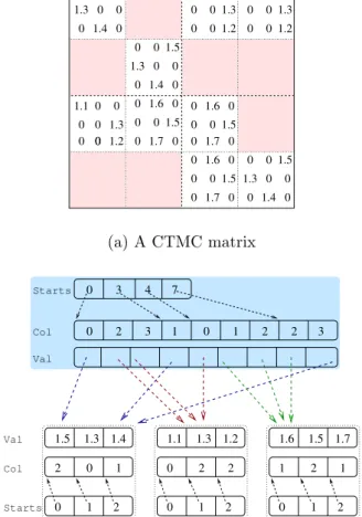
0 0 0 1.3 1.4 0 0 0 0 0 0 0 0 0 1.3 1.4 0 0 0 0 0 0 1.3 1.4 0 0 0 0 0 0 1.1 0 0 0 0 0 0 1.1 0 00 0 0 0 0 1.1 0 0 0 0 0 0 1.6 0 0 0 0 0 0 1.6 1.5 1.5 1.2 1.2 1.2 1.5 1.5 1.5 1.3 1.3 1.3 1.7 1.7 0 0 0 0 1.5 1.6 1.7 0 0 (a) A CTMC matrix Col Val Starts 1.5 2 0 1 2 0 1 1.3 1.4 1.1 0 1 2 2 2 1.3 1.2 1.6 1 0 1 2 2 1 1.5 1.7 0 Starts Col Val 0 2 1 0 1 2 2 3 0 3 4 7 3 (b) Modified MTBDD representation
Figure 1: A CTMC matrix and its representation as a modified MTBDD
its predecessors. It is highly configurable, and is en-tirely based on a fast, array-based storage, which al-lows effective decomposition, distribution, and manip-ulation of the data structure. Finally, the Gauss-Seidel method can be efficiently implemented using the mod-ified MTBDDs, which is not true for its predecessors; see [47,49], for serial Gauss-Seidel, and [43,64], for par-allel Gauss-Seidel implementations.
Figure 1 depicts a 12×12 CTMC matrix and its representation as a (modified) MTBDD. Note the two-layered storage. MTBDDs store the diagonal elements of a CTMC matrix separately as an array, in order to preserve structure in the symbolic representation of the CTMC. Hence, the diagonal entries of the matrix in Figure 1(a) are all zero. The matrix is divided into 42 blocks, where some of the blocks are zero (shown as shaded in pink). Each block in the matrix is of size 3×3. The blocks in the matrix are shown of equal size. However, usually, an MTBDD yields matrix blocks of unequal and varying sizes.
The information for the nonzero blocks in the ma-trix is stored in the MSR format, using the three arrays
Starts,Col, andVal(see the top part of Figure 1(b)). The arrayColstores the column indices of the matrix blocks in a row-wise order, and thei-th element of the arrayStartscontains the index inColof the beginning of thei-th row. The arrayValkeeps track of the actual block storage in the bottom layer of the data structure. Each distinct matrix block is stored only once, using the MSR format; see bottom of Figure 1(b). The mod-ified MTBDDs actually use the compact MSR format for both the top and the bottom layers of the storage. For simplicity, we used the (standard) MSR scheme in the figure.
The modified MTBDD can be configured to tailor the time and memory properties of the data structure according to the needs of the solution methods. This is explained as follows. An MTBDD is a rooted, di-rected acyclic graph, comprising two types of nodes:
terminal, andnon-terminal. Terminal nodes store the actual matrix entries, while non-terminal nodes store integers, called offsets. These offsets are used to com-pute the indices for the matrix entries stored in the terminal nodes. The nodes which are used to compute the row indices are calledrow nodes, and those used to compute the column indices are called column nodes. A level of an MTBDD is defined as an adjacent pair of rank of nodes, one for row nodes and the other for column nodes. Each rank of nodes in MTBDD corre-sponds to a distinct boolean variable. The total num-ber of levels is denoted byltotal. Descending each level
of an MTBDD splits the matrix into 4 submatrices. Therefore, descending lb levels, for some lb < ltotal,
gives a decomposition of a matrix intoP2blocks, where
P = 2lb. The decomposition of the matrix shown in Figure 1(a) into 16 blocks is obtained by descending 2 levels in the MTBDD, i.e. by usinglb= 2. The number
of block levelslbcan be computed usinglb=k×ltotal,
for somek, with 0≤k <1. A larger value for k(with some threshold value below 1) typically reduces the memory requirements to store a CTMC matrix, how-ever, it yields larger number of blocks for the matrix. A larger number of blocks usually can worsen perfor-mance for out-of-core and parallel solutions.
In [49], the author used lb = 0.6×ltotal for the
in-core solutions, andlb= 0.4×ltotalfor the out-of-core
solution. A detailed discussion of the affects of the pa-rameter lb on the properties of the data structure, a
comprehensive description of the modified MTBDDs, and the analyses of its in-core and out-of-core imple-mentations can be found in [49].
2.9 Case Studies
We have used three widely used CTMC case studies to benchmark our parallel algorithm. The case stud-ies have been generated using the tool PRISM [41]. First among these is the flexible manufacturing system
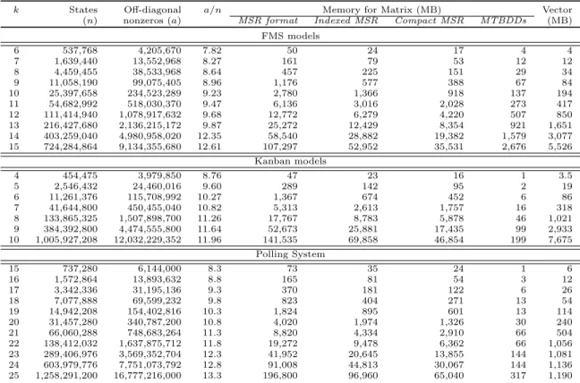
Table 1: Comparison of Storage Methods
k States Off-diagonal a/n Memory for Matrix (MB) Vector
(n) nonzeros (a) MSR format Indexed MSR Compact MSR MTBDDs (MB)
FMS models 6 537,768 4,205,670 7.82 50 24 17 4 4 7 1,639,440 13,552,968 8.27 161 79 53 12 12 8 4,459,455 38,533,968 8.64 457 225 151 29 34 9 11,058,190 99,075,405 8.96 1,176 577 388 67 84 10 25,397,658 234,523,289 9.23 2,780 1,366 918 137 194 11 54,682,992 518,030,370 9.47 6,136 3,016 2,028 273 417 12 111,414,940 1,078,917,632 9.68 12,772 6,279 4,220 507 850 13 216,427,680 2,136,215,172 9.87 25,272 12,429 8,354 921 1,651 14 403,259,040 4,980,958,020 12.35 58,540 28,882 19,382 1,579 3,077 15 724,284,864 9,134,355,680 12.61 107,297 52,952 35,531 2,676 5,526 Kanban models 4 454,475 3,979,850 8.76 47 23 16 1 3.5 5 2,546,432 24,460,016 9.60 289 142 95 2 19 6 11,261,376 115,708,992 10.27 1,367 674 452 6 86 7 41,644,800 450,455,040 10.82 5,313 2,613 1,757 16 318 8 133,865,325 1,507,898,700 11.26 17,767 8,783 5,878 46 1,021 9 384,392,800 4,474,555,800 11.64 52,673 25,881 17,435 99 2,933 10 1,005,927,208 12,032,229,352 11.96 141,535 69,858 46,854 199 7,675 Polling System 15 737,280 6,144,000 8.3 73 35 24 1 6 16 1,572,864 13,893,632 8.8 165 81 54 3 12 17 3,342,336 31,195,136 9.3 370 181 122 6 26 18 7,077,888 69,599,232 9.8 823 404 271 13 54 19 14,942,208 154,402,816 10.3 1,824 895 601 13 114 20 31,457,280 340,787,200 10.8 4,020 1,974 1,326 30 240 21 66,060,288 748,683,264 11.3 8,820 4,334 2,910 66 504 22 138,412,032 1,637,875,712 11.8 19,272 9,478 6,362 66 1,056 23 289,406,976 3,569,352,704 12.3 41,952 20,645 13,855 144 1,081 24 603,979,776 7,751,073,792 12.8 91,008 44,813 30,067 144 1,136 25 1,258,291,200 16,777,216,000 13.3 196,800 96,960 65,040 317 1,190
(FMS) of Ciardo and Tilgner [13], who used this model to benchmark their decomposition approach for the so-lution of large stochastic reward nets (SRNs), a class of Markovian stochastic Petri nets [54]. The FMS model comprises three machines which process different types of parts. One of the machines may also be used to as-semble two parts into a new type of part. The total number of parts in the system is kept constant. The model parameter k denotes the maximum number of parts which each machine can handle. Second CTMC model is the Kanban manufacturing system [12], again due to Ciardo and Tilgner. The authors used the Kan-ban model to benchmark their Kronecker-based solu-tion of CTMCs. The Kanban model comprises four machines. The model parameterkrepresents the max-imum number of jobs that may be in a machine at one time. Finally, third CTMC model is the cyclic server polling system of Ibe and Trivedi [33]. The Polling system consists of k stations or queues and a server. The server polls the stations in a cycle to determine if there are any jobs in the station for processing. We will abbreviate the names of these case studies to “FMS”, “Kanban” and “Polling” respectively.
Table 1 gives statistics for the three CTMC models, and compares storage requirements for MSR, indexed MSR, compact MSR and (modified) MTBDDs. The first column in the table gives the model parameterk;
the second and third columns list the resulting num-ber of reachable states and the numnum-ber of transitions respectively. The number of states and the number of transitions increase with an increase in the parameter
k. The fourth column (a/n) gives the average number of the off-diagonal nonzero entries per row, an indica-tion of the matrix sparsity. The largest model reported in the table is Polling (k= 25) with over 12.58 billion states and 16.77 billion transitions.
Columns 5−8 in Table 1 give the (RAM) storage requirements for the CTMC matrices (excluding the storage for the diagonal) in MB for the four data struc-tures. The indexed MSR format does not require RAM to store the diagonal for the iteration phase (see Sec-tion 2.7.3). The (standard) MSR format stores the diagonal as an array of 8nbytes. The compact MSR scheme and the (modified) MTBDDs store the diago-nal entries as short int (2 Bytes), and therefore require an array of 2nbytes for the diagonal storage. The last column lists the memory required to store a single iter-ation vector of doubles (8 bytes) for the solution phase. Note in Table 1 that the storage for the three ex-plicit schemes is dominated by the memory required to store the matrix, while the memory required to store vector dominates the storage for the implicit scheme (MTBDD). Note also that the memory require-ments for the three explicit methods are independent
of the case studies used, while for MTBDDs (implicit method), memory required to store CTMCs is heavily influenced by the case studies used. Finally, we observe that the memory required to store some of the Polling CTMC matrices is the same (e.g., k = 23, 24). This is possible in case of MTBDDs because these exploit structure in models which can possibly lead to similar amount of storage for different sizes of CTMCs.
The storage listed for the MTBDDs in Table 1 needs further clarification. We have mentioned earlier in Sec-tion 2.8 that the memory requirements for the MTB-DDs can be configured using the parameter lb. The
memories for the MTBDD listed in the table are given
for lb = 0.4×ltotal. For parallel solutions, we believe
that this heuristic gives an adequate compromise be-tween the amount of memory required for matrix stor-age and the number of blocks in the matrix. However, this issue needs further analysis and will be considered in our future work.
3 A Block Jacobi Algorithm
Iterative algorithms for the solution of linear equation system Ax=b perform matrix computations in row-wise or column-row-wise fashion. Block-based formulations of the iterative methods which perform matrix compu-tations on block by block basis usually turn out to be more efficient.
We have described Jacobi iterative method in Sec-tion 2.2. In this secSec-tion, we present a block Jacobi algorithm for the solution of the linear equation sys-tem Ax = b. Using this algorithm, we will be able to compute the steady-state probabilities of a CTMC, with A = QT, x = πT, and b = 0. In the
follow-ing, we briefly explain theblock iterative methods, and subsequently go on to describe our block Jacobi algo-rithm. For further details on block iterative methods, see e.g. [61, 15].
A block iterative method partitions a system of lin-ear equations into a certain number of blocks or sub-systems. We consider a decomposition of the state space S of a CTMC into P contiguous partitions
S0, . . . , SP−1, of sizes n0, . . . , nP−1, such that n =
PP−1
i=0 ni. We additionally definenmax= max{ni|0≤
i < P}, the size of the largest CTMC partition (or
equally, the largest block of the vector x). Using this decomposition of the state space, matrixAcan be di-vided into P2 blocks, {A
ij | 0 ≤ i, j < P}, where
the rows and columns of blockAij correspond to the
states inSiandSj, respectively, i.e. blockAij is of size
ni×nj. Therefore, forP = 4, the system of equations
Ax=bcan be partitioned as follows.
A00 A01 A02 A03 A10 A11 A12 A13 A20 A21 A22 A23 A30 A31 A32 A33 X0 X1 X2 X3 = B0 B1 B2 B3 (9)
Algorithm 1 A (Serial) Block Jacobi Algorithm
ser block Jac(A, b, x, P, n[ ], ε){
1. varx, Y, k˜ ←0, error←1.0, i, j 2. while(error> ε) 3. k←k+ 1 4. for( 0≤i < P) 5. Y ←Bi 6. for( 0≤j < P;j6=i) 7. Y ←Y −AijX (k−1) j
8. vec update Jac(Xi(k), Aii, X
(k−1)
i , Y, n[i])
9. computeerror 10. Xi(k−1)←Xi(k)
}
Using a partitioning of the systemAx=b, as described above, a block iterative method solvesPsub-systems of linear equations, of sizesn0, . . . , nP−1, within aglobal
iterative structure. If the Jacobi iterative method is employed as the global structure, it is called the block Jacobimethod. From Equations (1) and (9), the block Jacobi method for the solution of the system Ax=b
is given by: AiiX (k) i =Bi− X j6=i Aij X (k−1) j , (10)
for alli, 0≤i < P, whereXi(k),Xi(k−1)andBiare the
i-th blocks of vectorsx(k),x(k−1)andb respectively. Consequently, in thei-th of the totalP phases of the
k-th iteration of the block Jacobi iterative method, we solve Equation (10) forXi(k). These sub-systems can be solved using either direct or iterative methods. It is not necessary even to use the same method to solve each sub-system. If iterative methods are used to solve these sub-systems then we may have several inneriterative methods, within a global or outer iterative method. Moreover, each of theP sub-systems of equations can receive either a fixed or varying number ofinner iter-ations. The block iterative methods which employ an inner iterative method typically require fewer (outer) iterations, provided multiple (inner) iterations are ap-plied to the sub-systems. However, a consequence of multiple inner iterations is that each outer iteration will require more work. Note that applying one Jacobi iteration on each sub-system in the global Jacobi it-erative structure reduces the block Jacobi method to the standard Jacobi method, i.e., gives a block-based formulation of the (standard) Jacobi iterative method. Algorithm 1 gives a block Jacobi algorithm for the solution of the system Ax = b. The algorithm,
ser block Jac(·), accepts the following parameters as input: the references to matrix A and the vector b; the reference to the vectorx, which contains an initial
approximation for the iteration vector; the number of partitionsP; the vectorn[ ]; and, a precision value for
the convergence test, ε. The vector n[ ] is of size P,
and itsi-th element contains the size of thei-th vector block. According to the notation introduced earlier for the block methods,n[i] equalsni.
The local vectors and variables for the algorithm are declared, and initialised on line 1. The vectorsxand ˜x
are used for the two iteration vectors,x(k−1)andx(k), respectively. The notation used for the block methods applies to the algorithm: Xi(k),Xi(k−1)andBi are the
i-th blocks of vectorsx(k),x(k−1)andb, respectively.
Each iteration of the algorithm consists ofP phases of computations (see the outer for loop given by lines 4−8). Thei-th phase updates the elements from the i-th block (Xi) of the iteration vector, using the
entries from thei-th row of blocks inA, i.e.,Aij for all
j, 0≤j < P. There are two main computations
per-formed in each of thePphases: the computations given by lines 6−7, where matrix-vector products (MVPs) are accumulated for all the matrix blocks of the i-th block row, except the diagonal block (i.e.,i6=j); and the computation given by line 8, which invokes the function vec update Jac(·) to update the i-th vector block.
The function vec update Jac(·) uses the Jacobi method to update the iteration vector blocks, and is defined by Algorithm 2. In the algorithm, Xi[p]
de-notes thep-th entry of the vector blockXi, andAii[p,q]
denotes the (p, q)-th element of the diagonal blockAii.
Note that line 3 in Algorithm 2 updatesp-th element of
Xi(k)by accumulating the product of the vectorXi(k−1)
and thep-th row of the blockAii.
Algorithm 2 A Jacobi (inner) Vector Update
vec update Jac(Xi(k), Aii, X
(k−1) i , Y, n[i] ){ 1. varp, q 2. for( 0≤p < n[i]) 3. Xi(k)[p]←Aii[p,p]−1(Y[p]− X q6=p Aii[p,q]Xi(k−1)[q]) } 3.1 Memory Requirements
Algorithm 1 requires storage for matrix A. To obtain an efficient implementation, the matrix must be stored in a format such that the matrix elements can be ac-cessed in a block-row-wise fashion. Furthermore, the storage format should allow row-wise access to each block of the matrix. In addition to the matrix, the block Jacobi algorithm requires two arrays to store the iteration vectors, each of size n. Another array Y of sizenmaxis required to accumulate the MVPs on line 7
of the algorithm.
4 Parallelisation
We begin this section with a brief introduction to some of the issues in parallel computing in the context of iter-ative methods. Subsequently, we describe our parallel Jacobi algorithm and its implementation.
The design of parallel algorithms involves partition-ingof the problem – the identification and the specifi-cation of the overall problem as a set of tasks that can be performed concurrently. A goal when partitioning a problem into several tasks is to achieve loadbalanc-ing, such that no process waits for another while car-rying out individual tasks. The communication among processes is usually expensive and hence it should be minimised, wherever possible, and overlapped with the computations. These goals may be at odds with one another. Hence, one should aim to achieve a good com-promise between these conflicting demands.
Some computational problems naturally possess high degree of parallelism for concurrent scheduling, for ex-ample, the Jacobi iterative method. We know from Section 2.2, that in the Jacobi method, the order in which the linear equations are updated is irrelevant, since Jacobi treats them independently. The elements of the iteration vector, therefore, can be updated con-currently. Some problems, however, are inherently se-quential. The Gauss-Seidel iterative method is a such example. It uses the most recently available approx-imation of the iteration vector (see Section 2.3). For sparse matrices, however, it is possible to parallelise the Gauss-Seidel method usingwavefront or multicoloring
techniques.
Multicolor ordering and wavefront techniques have been in use to extract and improve parallelism in iterative solution methods. For sparse matrices, these techniques can be used to reorder the iterative computations such that the computations of unrelated vector elements can be carried out in parallel. Thewavefront
technique partitions a linear equation system into wavefronts. The unknown elements within a wavefront can be computed asynchronously by assigning these to multiple processors. Mul-ticolor orderingtechniques can take this further if the aim is to maximise parallelism. The ordering refers to a technique of col-oring the nodes of a graph associated with a matrix in such a way that no two adjacent nodes have the same color. The aim herein is to minimise the number of colors, and finding such min-imum colorings is a combinatorial problem of exponential com-plexity. For iterative methods, however, simple heuristics can provide acceptable colorings. A Gauss-Seidel iteration, precon-ditioned with multicolor ordering, can proceed in phases equal to the number of colors used in the ordering, while computation of the unknown elements within a color can proceed in parallel. Note that the solution of a permuted system with parallel Gauss-Seidel does not always result in improved overall performance, because it is possible that the Jacobi method delivers better per-formance by exploiting the natural ordering of a particular sparse system. Furthermore, as a result of multicolor ordering, the rate of convergence for the permuted matrix is likely to decrease. For further details, see e.g. [4, 58].
Note 4.1: Wavefronts, Multicoloring, and Gauss-Seidel
Parallelising the iterative methods involves decom-position of the matrix and the solution vector into blocks, such that the individual partitions can be com-puted concurrently. A number of schemes have been in use to partition a system. The row-wise block-striped
partitioning scheme is one such example. The scheme decomposes a matrix into blocks of complete rows, and each process is allocated one such block. The vector is also decomposed into blocks of corresponding sizes.
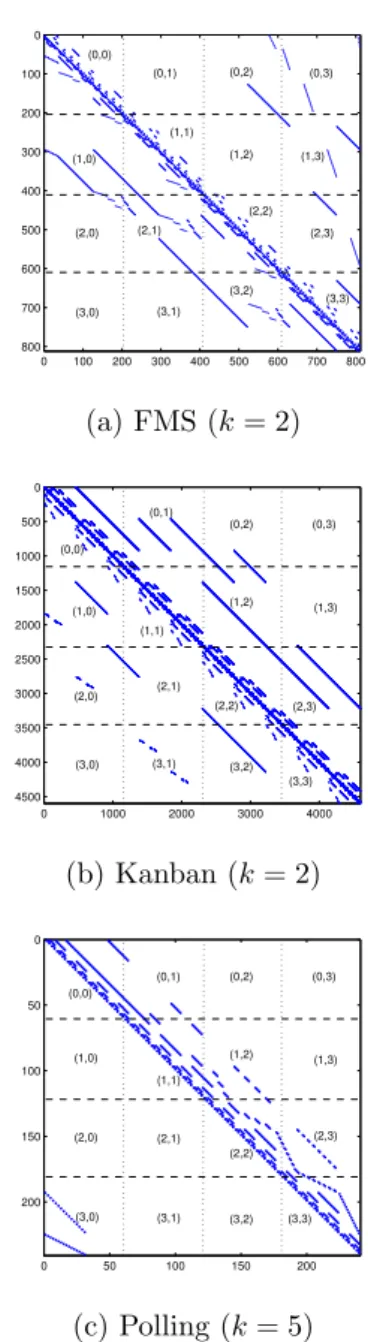
Figure 2 plots the off-diagonal nonzero entries for three CTMC matrices, one from each of the three case studies. The figure also depicts the row-wise block-striped partitioning for the three matrices. The ma-trices have been row-wise decomposed into four blocks (see dashed lines), for distribution to a total of four processes. Process p keeps all the (p, q)-th matrix blocks, for all q. Using this matrix partitioning, the iteration vector can also be divided into four blocks of corresponding sizes. Process p will be allocated, and made responsible to iteratively compute the p-th vec-tor block. Note that, to compute thep-th vector block, processpwill require access to all theq-th blocks such that Apq 6= 0. Hence, we say that the p-th block for
a processpis itslocal block, while all theq-th blocks,
q6=p, are theremoteblocks for the process.
Matrix sparsity usually leads to poor loadbalancing. For example, balancing the computational load for par-allel processes participating in the computations may not be easy, and/or the processes may have different communication needs. Sparsity in matrix also leads to high communication to computation ratio. For these reasons, parallelising sparse matrix computations com-pared to dense matrices is usually considered hard. However, it may be possible, sometimes, to exploit
sparsity pattern of a matrix. For example,bandedand
block-tridiagonalmatrices possess a fine degree of par-allelism in their sparsity patterns. This is explained further in the following paragraph, using the CTMC matrices from the three case studies.
Consider again Figure 2, which also shows the spar-sity pattern for three CTMC matrices. The sparspar-sity pattern for all the matrices of a particular CTMC model is similar. Note in the figure that both FMS and Kanban matrices have irregular sparsity patterns, while the Polling matrix exhibits a regular pattern. Most of the nonzero entries in the Polling matrix are confined to a band on top of the principal diagonal, except those relatively few nonzero entries which are located within the lower left block of the matrix. If the matrix is partitioned among 4 processes, as shown in the figure, communication is only required in be-tween two neighbouring processes. Furthermore, since most of the nonzero entries are located within the di-agonal blocks, relatively few elements of the remote vector blocks are required. It has been shown in [48], that a parallel algorithm tailored in particular for the
0 100 200 300 400 500 600 700 800 0 100 200 300 400 500 600 700 800 (0,0) (0,1) (0,2) (0,3) (1,0) (1,1) (1,2) (1,3) (2,0) (2,1) (2,2) (2,3) (3,0) (3,1) (3,2) (3,3) (a) FMS (k= 2) 0 1000 2000 3000 4000 0 500 1000 1500 2000 2500 3000 3500 4000 4500 (0,0) (0,1) (0,2) (0,3) (1,0) (1,1) (1,2) (1,3) (2,0) (2,1) (2,2) (2,3) (3,0) (3,1) (3,2) (3,3) (b) Kanban (k= 2) 0 50 100 150 200 0 50 100 150 200 (0,0) (0,1) (0,2) (0,3) (1,0) (1,1) (1,2) (1,3) (2,0) (2,1) (2,2) (2,3) (3,0) (3,1) (3,2) (3,3) (c) Polling (k= 5)
Figure 2: Sparsity pattern for three CTMC matrices selected from the three case studies
sparsity pattern of the Polling matrices achieves signif-icantly better performance than for arbitrary matrices. The parallel algorithm presented in this paper does not
explicitly exploit sparsity patterns in matrices. How-ever, we will see in Section 5 that the performance of the parallel algorithm for the Polling matrices is better than for the other two case studies.
4.1 The Parallel Algorithm
Algorithm 3 presents a high-level description of our parallel Jacobi iterative algorithm. It is taken with some modifications from our earlier work [48]. The algorithm employs the Jacobi iterative method for the
Algorithm 3 A Parallel Jacobi for Processp
par block Jac( ˇAp, Dp, Bp, Xp, T, Np, ε){
1. varX˜p, Z, k←0, error←1.0, q, h, i 2. while(error> ε) 3. k←k+ 1 4. h= 0 5. for( 0≤q < T;q6=p) 6. if( ˇApq6=0) 7. send(requestXq, q) 8. h=h+ 1 9. Z←Bp−AˇppX (k−1) p 10. while(h >0)
11. if( probe(message) ) 12. if(message=requestX
p) 13. send(Xp, q) 14. else 15. receive(Xq, q) 16. Z←Z−AˇpqX (k−1) q 17. h=h−1 18. serve(Xp,requestXp) 19. for( 0≤i < Np) 20. Xp(k)[i]←Dp[i]−1Z[i]
21. computeerror collectively }
solution of the system ofnlinear equations, of the form
Ax =b. The steady-state probabilities can be calcu-lated using this algorithm withA=QT,x=πT, and
b = 0. The algorithm uses the single program mul-tiple data (SPMD) paradigm – all the nodes execute the same binaries but operate on different sets of data. Note that the design of Algorithm 3 is influenced by the fact that MPI is thread-unsafe, otherwise concurrency in the algorithm can easily be improved.
We store the off-diagonal CTMC matrix using the (modified) MTBDDs [49, 47] (see Section 2.8). The di-agonal entries of the matrix are stored separately as an array. For convenience in this discussion, we addition-ally introduce: the matrix ˇA, which contains the off-diagonal elements ofA, with ˇaii = 0, for all 0≤i < n;
and the diagonal vectord, with the entriesdi=aii.
Consider a total of T processes2. Algorithm 3 as-sumes that the off-diagonal matrix ˇAis row-wise block-striped partitioned into T contiguous blocks of com-plete rows, of sizes N0, . . . , NT−1, such that n =
PT−1
p=0 Np. A such partitioning is depicted in Figure 2.
Processpis allocated a matrix block of sizeNp×n, with
all the rows numbering fromPp−1
q=0Nq to
Pp
q=0Nq−1.
Moreover, each row of blocks is further divided intoT
blocks such that thep-th process keeps all the blocks,
2In this paper, we have used process, rather than processor
or node, because it has a more general meaning.
ˇ
Apq, 0 ≤q < T. We will use ˇAp to denote the block
row containing all the blocks ˇApq.
Using the same partitioning as for the matrix, the it-eration vectorx, and the diagonal vectord, are divided intoT blocks each, of the sizes,N0, . . .NT−1. Process
p keeps the p-th blocks, Xp and Dp, of the two
vec-tors and is responsible for updating the iteration vector block Xp during each iteration. As mentioned earlier,
we will refer to the blockXp as thelocalblock for
pro-cesspbecause it does not require communication while computing the MVP ˇAppX
(k−1)
p . Conversely, all the
blocks Xq, q6=p, are the remoteblocks for process p
because computing ˇApqX
(k−1)
q requires blocksXq(k−1)
which are owned by the other processes.
The algorithm, par block Jac(·), accepts the follow-ing parameters as input: the reference to thep-th row of the off-diagonal matrix blocks, ˇAp; the reference to
thep-th diagonal block,Dp; the reference to the block
Bp which is zero in our case; the reference to the
vec-tor block Xp which contains an initial approximation
for the iteration vector block; the total number of pro-cessesT; the constantNp, which gives the number of
entries in the vector block Xp; and a precision value
for the convergence test,ε.
The vectors and variables local to the algorithm are declared, and initialised on line 1. The vectors Xp
and ˜Xp are used in the algorithm for the two iteration
vectors,Xp(k−1), Xp(k), respectively.
In each Jacobi iteration, given in Algorithm 3, the main task of process p is to accumulate the MVPs,
ˇ
ApqXq, for all q (see lines 9 and 16). These MVPs
are accumulated using the vector Z. Having accom-plished this, the local block Xp for process p can be
computed using the vectorsZ andDp (lines 19−20).
Since processpdoes not have access to all the blocks
Xq, except for q=p, it sends requests to all the
pro-cesses numbered qfor the blocksXq corresponding to
the nonzero matrix blocks ˇApq (lines 4−8). The
pro-cess computes the MVP for local block on line 9. Sub-sequently, the process iteratively probes for the mes-sages from other processes (lines 10−17). The block
Xp is sent to processqif a request from the process is
received (lines 12−13)). If processqhas sent the block
Xq, the block is received and the MVP for this remote
block is computed (lines 15−17). Once all the MVPs have been accumulated, processpwaits and serves for any remaining requests for Xp from other processes
(line 18), and then goes on to update its local block
Xp for the k-th iteration (lines 19−20). Finally, on
line 21, all the processes collectively perform the test for convergence – each process pcomputes error us-ing the criteria given by Equation (8), for 0≤i < Np,
and the maximum of all these errors is determined and communicated to all the processes.
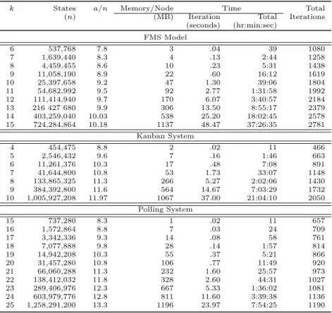
Table 2: Solution Results for Parallel Execution on 24 Nodes
k States a/n Memory/Node Time Total
(n) (MB) Iteration Total Iterations
(seconds) (hr:min:sec) FMS Model 6 537,768 7.8 3 .04 39 1080 7 1,639,440 8.3 4 .13 2:44 1258 8 4,459,455 8.6 10 .23 5:31 1438 9 11,058,190 8.9 22 .60 16:12 1619 10 25,397,658 9.2 47 1.30 39:06 1804 11 54,682,992 9.5 92 2.77 1:31:58 1992 12 111,414,940 9.7 170 6.07 3:40:57 2184 13 216 427 680 9.9 306 13.50 8:55:17 2379 14 403,259,040 10.03 538 25.20 18:02:45 2578 15 724,284,864 10.18 1137 48.47 37:26:35 2781 Kanban System 4 454,475 8.8 2 .02 11 466 5 2,546,432 9.6 7 .16 1:46 663 6 11,261,376 10.3 17 .48 7:08 891 7 41,644,800 10.8 53 1.73 33:07 1148 8 133,865,325 11.3 266 5.27 2:02:06 1430 9 384,392,800 11.6 564 14.67 7:03:29 1732 10 1,005,927,208 11.97 1067 37.00 21:04:10 2050 Polling System 15 737,280 8.3 1 .02 11 657 16 1,572,864 8.8 7 .03 24 709 17 3,342,336 9.3 14 .08 58 761 18 7,077,888 9.8 28 .14 1:57 814 19 14,942,208 10.3 55 .37 5:21 866 20 31,457,280 10.8 106 .77 11:49 920 21 66,060,288 11.3 232 1.60 25:57 973 22 138,412,032 11.8 328 2.60 44:31 1027 23 289,406,976 12.3 667 5.33 1:36:02 1081 24 603,979,776 12.8 811 11.60 3:39:38 1136 25 1,258,291,200 13.3 1196 23.97 7:54:25 1190
converge with the Jacobi iterative method. For Kan-ban matrices, hence, on line 20, we apply additional (JOR) computations given by Equation (3).
4.1.1 Implementation Issues
For each processp, Algorithm 3 requires two arrays of
Npdoubles to store its share of the vectors for the
iter-ations,k−1 andk. Another array of at mostnmax(see
Section 3) doubles is required to store the blocks Xq
received from process q. Moreover, each process also requires storage of its share of the off-diagonal matrix
ˇ
A, and the diagonal vector Dp. The number of the
distinct values in the diagonal of the CTMC matrices considered is relatively small. Therefore, storage ofNp
short int indices to an array of the distinct values is required, instead ofNp doubles.
Note also that the modified MTBDD partitions a CTMC matrix intoP2blocks for someP, as explained
in Section 3. For the parallel algorithm, we make the additional restrictions thatT ≤P, which implies that each process is allocated with at least one row of MTBDD blocks. In practice, however, the numberP
is dependent on the model and is considerably larger than the total number of processesT.
5 Experimental Results
In this section, we analyse performance for Algorithm 3 using its implementation on a processor bank. The pro-cessor bank is a collection of loosely coupled machines. It consists of 24 dual-processor nodes. Each node has 4GB of RAM. Each processor is anAMD Opteron(TM) Processor 250 running at 2400MHz with 1MB cache. The nodes in the processor bank are connected by a pair ofCisco 3750G-24Tswitches at 1Gbps. Each node has dualBCM5703X Gb NICs, of which only one is in use. The parallel Jacobi algorithm is implemented in C language using the MPICH implementation [27] of the message passing interface (MPI) standard [22]. The results reported in this section were collected without an exclusive access to the processor bank.
We analyse our parallel implementation with the help of the three benchmark CTMC case studies: FMS, Kanban and Polling systems. These have been intro-duced in Section 2.9. We use the PRISM tool [41] to generate these models. For our current purposes, we have modified version 1.3.1 of the PRISM tool. The modified tool generates the underlying matrix of a CTMC in the form of the modified MTBDD (see Sec-tion 2.8). It decomposes the MTBDD into partiSec-tions, and exports the partitions for parallel solutions.
0 150 300 450 600 750 900 1050 1200 1400 0 5 10 15 20 25 30 35 40 45 50 States (millions)
Time per iteration (seconds)
FMS Kanban Polling
Figure 3: Comparison of the execution times per it-eration for the three case studies (plotted against the number of states)
time and space statistics reported in this table are col-lected by executing the parallel program on 24 proces-sors, where each processor pertains to a different node. For each CTMC, the first three columns in the table report the model statistics: column 1 gives the values for the model parameterk, column 2 lists the resulting number of reachable states (n) in the CTMC matrix, and column 3 lists the average number of nonzero en-tries per row (a/n). Column 4 reports the maximum of the memories used by the individual processes. The last three columns, 5−7, report the execution time per iteration, the total execution time for the steady-state solution, and the number of iterations, respec-tively. All reported run times are wall clock times. For FMS and Polling CTMCs, the reported iterations are for the Jacobi iterative method, and for Kanban, the column gives the number of JOR iterations (Kanban matrices do not converge with Jacobi). The iterative methods were tested for the convergence criterion given by Equation (8) forε= 10−6.
In Table 2, the largest CTMC model for which we obtain the steady-state solution is the Polling system (k = 25). It consists of over 1258 million reachable states. The solution for this model used a maximum of 1196MB RAM per process. It took 1190 Jacobi it-erations, and 7 hours, 54 minutes, and 25 seconds, to converge. Each iteration for the model took an av-erage of 23.97 seconds. The largest Kanban model (k = 10) which was solved contains more than 1005 million states. The model required 2050 JOR itera-tions, and approximately 21 hours (less then a day) to converge, using no more than 1.1GB per process. The largest FMS model which consists of over 724 million states, took 2781 Jacobi iterations and less than 38 hours (1.6 days) to converge, using at most 1137MB of memory per process.
A comparison of the solution statistics for the three models in Table 2 reveals that the Polling CTMCs of-fer the fastest execution times per iteration, the FMS matrices exhibit the slowest times, and the times per
1 4 8 12 16 20 24 32 40 48 0 5 10 15 20 25 30 35 40 45 50 55 60 Processes
Time per iteration (seconds)
FMS(k=12) FMS(k=15)
(a) FMS (times per iteration)
1 4 8 12 16 24 32 40 48 0 5 10 15 20 25 30 35 40 45 50 60 Processes
Time per iteration (seconds)
Kanban(k=8) Kanban(k=10)
(b) Kanban (times per iteration)
1 4 8 12 16 24 32 40 48 0 4 8 12 16 20 24 28 32 36 60 Processes
Time per iteration (seconds)
Polling(k=22) Polling(k=25)
(c) Polling (times per iteration)
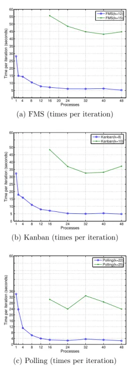
Figure 4: Time per iteration against the number of processes for six CTMCs, two from each case study iteration for the Kanban CTMCs lie in between. Note also that the convergence rate for the Polling CTMCs is the highest (e.g. 1190 iterations) among the three types of models, while for FMS, it is the lowest (2781 iterations). To further explore the relative performance of our parallel solution for the three case studies, we plot the run times per iteration for the three exam-ple CTMCs against the number of states in Figure 3. In the figure, the magnitudes of the individual slopes for the three models expose their comparative speeds. A potential cause for the differences in the perfor-mance lies in that the three models possess different
amount of structure. The FMS system is the least structured of the three models. Since an MTBDD ex-ploits model structure to produce a compact storage for CTMCs, models with less structure yield a larger MTBDD (see [49], Chapter 5, for a detailed discussion of the MTBDD). A larger MTBDD may require addi-tional overhead for its parallelisation. However, a more important and stronger cause for this behaviour is the differences in the sparsity patterns of the three mod-els; see Figure 2. Note in the figure that, among the three case studies, the FMS model exhibits the most ir-regular sparsity pattern. An irir-regular sparsity pattern can lead to load imbalance for computations as well as communications, and, as a consequence, can cause an overall worse performance.
We now analyse performance for the parallel solution with respect to the number of processes. In Figure 4, for the three case studies, we plot the execution times per iteration against the number of processes. We se-lect two models from each case study. One of these is the largest model solved for each case study; e.g., the Kanban (K= 10) model with 1005 million states. The execution times are collected for up to a maximum of 48 processes. For the larger models, however, run time are only collected for 16 or more processes due to their excessive RAM requirements. To explain the figure, we consider the FMS plots given in Figure 4(a), in partic-ular, the plot for the (smaller) FMS model (k = 12), which contains over 111 million states. As expected, the increase in the number of processes (from 1 to 24) causes a decrease in the time per iteration (from 28.18 to 6.07 seconds). However, there is a somewhat contin-ual drop in the value of the magnitude of the slope for the plot as it approaches the 24 process mark. Simi-larly, in Figure 4(a), the plot for the larger FMS model (k = 15, 724 million states) also shows a decrease in the execution times with an increase in the number of processes: increasing the processes from 16 to 24 brings the execution time from 55.63 seconds down to 48.47
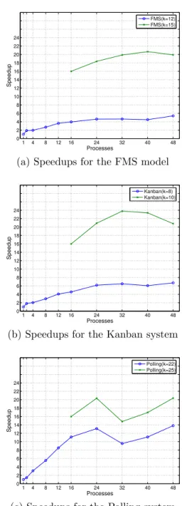
Perhaps speedup is the most common measure in practice for evaluating performance of parallel algorithms. It captures the relative benefits of solving a problem in parallel. Speedup may be defined as the ratio of the time taken to solve a problem using a single process to the time required to solve the same problem using a collection of T concurrent processes. For a fair com-parison, each parallel process must be given resources (CPU, RAM, I/O) identical to the resources given to the single pro-cess. Suppose, Time1 and TimeT are the times taken by the serial algorithm and the parallel algorithm onT processes, re-spectively. The speedupSpeedT is given byTime1/TimeT. The ideal speedup forT processes isT. Another measure to evaluate performance of parallel algorithms isefficiency, which is defined as the ratio of the speedup to the number of processes used, i.e.,
SpeedT/T. The ideal value for efficiency is 1, or 100%, although
superlinearspeedup can cause even higher values for efficiency.
Note 5.1: Speedup and Efficiency
1 4 8 12 16 24 32 40 48 0 2 4 6 8 10 12 14 16 18 20 22 24 Processes Speedup FMS(k=12) FMS(k=15)
(a) Speedups for the FMS model
1 4 8 12 16 24 32 40 48 0 2 4 6 8 10 12 14 16 18 20 22 24 Processes Speedup Kanban(k=8) Kanban(k=10)
(b) Speedups for the Kanban system
1 4 8 12 16 24 32 40 48 0 2 4 6 8 10 12 14 16 18 20 22 24 Processes Speedup Polling(k=22) Polling(k=25)
(c) Speedups for the Polling system
Figure 5: Speedup plotted against the number of pro-cesses for six CTMCs
seconds. However, for the larger model, the magni-tude of the slope is greater (at this point of the plot), implying a steeper drop in the execution time.
To further investigate the parallel performance, in Figure 5, we plot speedups for six CTMCs against the number of up to 48 processes. We use the same six CTMCs which were used in Figure 4. Consider in Fig-ure 5(b), the plot for the smaller Kanban model (k= 8, 133 million states). The plot shows that increasing the number of processes from 1 to 2 gives a speedup of 1.8, which equates to an efficiency of 0.90 or 90%. The plot, however, further reveals that a continual increase in