Cluster
著者
KOZAWA Yusuke, AMAGASA Toshiyuki, KITAGAWA
Hiroyuki
journal or
publication title
IEICE transactions on information and systems
volume
E97.D
number
4
page range
779-789
year
2014-04
権利
(C) 2014 The Institute of Electronics,
Information and Communication Engineers
URL
http://hdl.handle.net/2241/00122496
PAPER
Special Section on Data Engineering and Information ManagementProbabilistic Frequent Itemset Mining on a GPU Cluster
Yusuke KOZAWA†a),Nonmember, Toshiyuki AMAGASA††,Member,andHiroyuki KITAGAWA††,Fellow
SUMMARY Probabilistic frequent itemset mining, which discovers frequent itemsets from uncertain data, has attracted much attention due to inherent uncertainty in the real world. Many algorithms have been pro-posed to tackle this problem, but their performance is not satisfactory be-cause handling uncertainty incurs high processing cost. To accelerate such computation, we utilize GPUs (Graphics Processing Units). Our previous work accelerated an existing algorithm with a single GPU. In this paper, we extend the work to employ multiple GPUs. Proposed methods minimize the amount of data that need to be communicated among GPUs, and achieve load balancing as well. Based on the methods, we also present algorithms on a GPU cluster. Experiments show that the single-node methods real-ize near-linear speedups, and the methods on a GPU cluster of eight nodes achieve up to a 7.1 times speedup.
key words: GPU, uncertain databases, probabilistic frequent itemsets 1. Introduction
Uncertain data management is attracting considerable in-terest due to inherent uncertainty in real-world applications such as sensor-monitoring systems. For example, when an-alyzing purchasing behavior of customers using RFID sen-sors, there may be inaccurate sensor readings because of er-rors. In addition to this example, uncertain data take place in many situations. The major cause of uncertainty involves limitations of equipment, privacy concerns, or statistical methods such as forecasting. To deal with such uncertain data,uncertain databaseshave recently been developed [2]. In the area of uncertain data management, frequent itemset mining [3] from uncertain databases is one of the im-portant research issues. Since the uncertainty is represented by probability, this problem is calledprobabilistic frequent itemset mining. Many algorithms have been proposed to tackle probabilistic frequent itemset mining [6], [15], [17], [18]. However, existing algorithms suffer from performance problems because the computation of probability is highly time-consuming. It is thus necessary to accelerate this com-putation in order to handle large uncertain databases.
To this end, GPGPU (General-Purpose computing on Graphics Processing Unit) is an attractive solution. GPGPU refers to performing computation on GPUs (Graphics
Pro-Manuscript received July 12, 2013. Manuscript revised October 29, 2013.
†The author is with the Graduate School of Systems and In-formation Engineering, University of Tsukuba, Tsukuba-shi, 305– 8573 Japan.
††The authors are with the Faculty of Engineering, Informa-tion and Systems, University of Tsukuba, Tsukuba-shi, 305–8573 Japan.
a) E-mail: [email protected] DOI: 10.1587/transinf.E97.D.779
cessing Units), which are originally designed for processing 3D graphics. GPGPU has received much attention from not only the field of high performance computing but also many other fields such as data mining [5], [7], [12], [14], [16]. This is because GPUs have more than hundred processing units and can process many data elements with high parallelism. It is also known that GPUs are energy-efficient and have higher performance-to-price ratios than CPUs. In addition, because the GPU architecture is relatively simpler than the CPU architecture, GPUs have been evolving rapidly [20].
By leveraging such a promising processor, our previ-ous work [9] accelerated an algorithm of probabilistic fre-quent itemset mining. Meanwhile, GPU clusters, which are computer clusters where each node has one or more GPUs, have emerged as a powerful computing platform, such as HA-PACS,∗ TSUBAME2.0,∗∗ and Titan.∗∗∗ Thus, it is in-creasingly important to harness the power of multiple GPUs and GPU clusters. The utilization of multiple GPUs gives us further parallelism and larger memory spaces. However, employing multiple GPUs has the problem that each GPU has a separate memory space. If one GPU requires data that reside in another GPU, the data need to be communicated via PCI-Express bus. Since the PCI-Express latency is much higher than the GPU-memory latency, it is probable that the communication becomes a bottleneck. It is therefore desir-able to reduce data dependencies among data fragments on different GPUs.
This paper proposes multi-GPU methods that take into account the above concerns. First, we develop methods on a single node with multiple GPUs, and then we extend the methods to use a GPU cluster. The proposed methods re-duce data dependencies by distributing candidates of prob-abilistic frequent itemsets among GPUs. In addition, the methods consider load balancing, which is also an impor-tant issue to achieve scalability. Experiments show that the single-node methods realize near-linear speedups, and the methods on a GPU cluster of eight nodes achieve up to a 7.1 times speedup.
The rest of this paper is organized as follows. Section 2 explains preliminary knowledge of proposed methods. Then Sect. 3 describes our proposed methods that utilize multiple GPUs. The methods are empirically evaluated in Sect. 4. Section 5 reviews related work, and Sect. 6 concludes this
∗http://www.ccs.tsukuba.ac.jp/CCS/eng/
research-activities/projects/ha-pacs
∗∗http://www.gsic.titech.ac.jp/en/tsubame2 ∗∗∗http://www.olcf.ornl.gov/titan
paper.
2. Preliminaries
This section describes necessary knowledge to understand our proposed methods. Section 2.1 defines the problem that this paper deals with, i.e., probabilistic frequent item-set mining. Then a baseline algorithm [15] is explained in Sect. 2.2. The algorithm on a single GPU [9] is described in Sect. 2.3.
2.1 Probabilistic Frequent Itemsets
LetI be a set of all items. A set of itemsX ⊆ I is called anitemset, and ak-itemset means an itemset that contains
kitems. Anuncertain transaction databaseU is a set of
transactions, each of which is a triplet of an ID, an item-set, and anexistential probability. An existential probability stands for the probability that a transaction really exists in the database. Table 1 shows an example of uncertain trans-action database, where each row corresponds to a transac-tion.
Uncertain transaction databases are often interpreted withpossible worlds model. This model considers that an uncertain transaction database generates possible worlds. Each possible world is a distinct subset of the database and represents an instance of the database. For example, the database of Table 1 generates 16 possible worlds: ∅,{T1},
{T2},{T3},{T4},{T1,T2}, etc. Each possible world is
prob-abilistically generated according to the existential probabil-ities. For instance, the world{T1,T2}is generated with the
probability thatT1andT2exist, andT3andT4do not exist.
Hence the probability is 0.6·0.8·(1−0.5)·(1−0.3)=0.168. The concept of support is used to define conventional frequent itemsets. The support of an itemsetXis denoted as sup(X) and means the number of transactions that include the itemset X. In this settings, the itemset X is regarded as frequent if the support is at least a user-specified thresh-oldminsup. Although this definition works well for cer-tain transaction databases, another concept is necessary to deal with uncertain transaction databases, because the sup-port varies with possible worlds.
Since possible worlds are generated probabilistically, the distribution of support can be denoted by a probabil-ity mass function. The probabilprobabil-ity mass function of the support of an itemset X is called a Support Probability Mass Function (SPMF) fX. The function fX takes an
in-tegeri∈ {0,1, . . . ,|U|}, whereUis an uncertain transaction database. fX(i) represents the probability that the support of
Xequalsi.
An itemsetXis called aProbabilistic Frequent Itemset (PFI)if P(sup(X)≥minsup)= |U| i=minsup fX(i)≥minprob, (1)
whereUis an uncertain transaction database, andminsup
Table 1 An uncertain transaction database. ID Itemset Probability T1 {a, b, c} 0.6
T2 {a, b} 0.8
T3 {a, c, d} 0.5
T4 {a, b, c, d} 0.3
andminprob∈(0,1] are user-specified thresholds. Proba-bilistic frequent itemset miningis to extract all probabilistic frequent itemsets, given an uncertain transaction database,
minsup, andminprob. 2.2 pApriori Algorithm
Sun et al. [15] proposed a pApriori algorithm, which adapts the classical Apriori algorithm [4] to uncertain databases. The pApriori algorithm comprises two procedures:
1. Generating a set ofcandidate k-itemsetsCkfrom a set of (k−1)-PFIsLk−1
2. Extracting a set ofk-PFIsLkfromCk
The pApriori algorithm continues these procedures al-ternately with incrementingkby one until no additional PFIs are detected. Note that, in the beginning of the algorithm,
k’s value is one and candidate 1-itemsets are singletons that contain items in an input databaseU. Eventually the pApri-ori algpApri-orithm returns all the PFIs extracted fromU. 2.2.1 Generating Candidates
Candidates are generated in two phases: merging and prun-ing phases.
The merging phase checks whether pairs of (k− 1)-PFIs arejoinable: Two (k−1)-itemsetsXandYsatisfy the conditionX.item1=Y.item1∧ · · · ∧X.itemk−2=Y.itemk−2∧
X.itemk−1 < Y.itemk−1, where X.itemi denotes theith item
ofX.† IfXandYare joinable, a new candidatek-itemset is created as the union ofXandY. This candidate is stored to a set of candidatek-itemsetsCk.
The pruning phase prunes candidates using the follow-ing lemma [15]:
Lemma 1 (Anti-monotonicity). If an itemset X is a PFI, then any itemset X ⊂X is also a PFI.
The contraposition of this lemma yields that if any itemsetX ⊂Xis not a PFI, then the itemsetXis not a PFI either. Hence a candidatek-itemset can be pruned out when any size-(k−1) subset of the candidate is not contained in a set of (k−1)-PFIsLk−1. If the candidate can be pruned out, it is deleted fromCk.
2.2.2 Extracting Probabilistic Frequent Itemsets
In order to determine whether or not an itemset X is a PFI, the SPMF ofXneeds to be computed and assigned to
Eq. (1). However, a na¨ıve solution to compute SPMFs is considered to be intractable, because the number of possible worlds is exponentially large. To address this problem, Sun et al. [15] proposed two algorithms: dynamic-programming and divide-and-conquer approaches. They showed that the divide-and-conquer algorithm is more efficient.
Although the algorithm is able to compute SPMFs in
Onlogntime, it is still a time-consuming task. Thus, it is desirable to prune infrequent itemsets without computing the SPMFs. Let cnt(X) be the number of transactions that include an itemsetXin an uncertain transaction databaseU regardless of existential probabilities. Besides, let esup(X) be the expected value of sup(X). With the two values, Sun et al. proved two lemmas that enable us to prune candidates inO(n) time [15].
2.3 Single-GPU Parallelization
The single-GPU method [9] follows the pApriori algorithm and consists of generating candidates and extracting PFIs. Candidates are generated on a GPU by a parallel version of the algorithm described in Sect. 2.2.1. Then PFIs are ex-tracted with four steps: inclusion check, pruning, filtering, and computing SPMFs. For more details, readers are en-couraged to refer to the paper [9].
Inclusion check judges whether transactions include each candidate. Since the information that a transaction in-cludes a candidate can be represented by one bit, the result of inclusion check for a candidate is stored as an array of bit-strings, called aninclist. By using inclists of (k−1)-itemsets, inclusion check fork>1 can be processed fast. The inclist of ak-itemsetXis computed as bitwise AND operations be-tween two inclists of (k−1)-PFIs that are used to create the itemsetX.
In the pruning step, candidates are pruned by comput-ing the two values mentioned in Sect. 2.2.2. Then, non-pruned candidates become subject to the filtering step. For each candidate, this step filters out transactions that do not include the candidate, because such transactions do not con-tribute to the SPMF of the candidate. With this filtering, the number of transactions to compute the SPMF of an item-setXdecreases from|U|to cnt(X). The next step computes the SPMF of this candidate and the algorithm determines whether the candidate is a PFI or not.
3. Multi-GPU Parallelization
In a multi-GPU system, each GPU has a separate memory space. If data dependencies exist among GPUs, GPUs need to communicate with each other via PCI-Express bus. Thus it is important how to distribute data to be processed on GPUs, so that data dependencies are minimized.
Multi-GPU systems can be considered as a kind of distributed-memory systems. Meanwhile, there exists much work on frequent itemset mining for distributed-memory systems. Zaki [19] classified data-distribution schemes that existing algorithms employ into three: count distribution,
Algorithm 1:Prefix distribution
1 Initialization (k=1)
2 Inclusion check and pruning on the CPU
3 Distribute candidatesC1and transfer inclists to GPUs
4 Filtering and computing SPMFs on GPUs
5 Gather 1-PFIs from GPUs to the CPU 6 Distribution (k=2)
7 Generate candidate 2-itemsets on the CPU 8 Distribute the candidatesC2to GPUs by prefix
9 whilea set of candidatesCk∅do
10 //Inclusion check uses inclists of (k−1)-itemsets 11 Extractk-PFIs on GPUs
12 Gather thek-PFIs from GPUs to the CPU 13 Broadcast all thek-PFIs to GPUs 14 k←k+1
15 Generate candidatek-itemsets on GPUs
data distribution, and candidate distribution. In this paper, we propose methods employing the candidate-distribution scheme, because this scheme enables GPUs to compute SPMFs independently, unlike the other two schemes.
Section 3.1 describes methods on a single node equipped with multiple GPUs. Then, Sect. 3.2 extends the methods to use a GPU cluster.
3.1 Single-Node Methods 3.1.1 Prefix Distribution
We here describe an algorithm based on a na¨ıve candidate-distribution scheme. This algorithm is calledPrefix Distri-bution (PD), because the algorithm distributes candidates by exploiting the property that two candidates with diff er-ent prefixes are not joinable. Therefore if we partition can-didates with prefixes, GPUs can generate cancan-didates using their own PFIs. Algorithm 1 shows a pseudocode of PD. PD is divided into three phases: initialization, distribution, and loop phases.
In the initialization phase, PD extracts 1-PFIs. PD firstly generates candidate 1-itemsets from an input uncer-tain transaction database, and then conducts inclusion check and pruning on the CPU in Line 2. By processing inclu-sion check and pruning on the CPU rather than on GPUs, the amount of data transfer to GPUs reduces, because the database is unnecessary in later iterations. Although inclu-sion check and pruning are performed individually in the single-GPU method, because it is more suitable for GPU’s architecture, these operations can be executed simultane-ously on the CPU. Thus PD performs these two operations at the same time. Non-pruned candidates are evenly distributes to GPUs (Line 3). Inclists of all the non-pruned candidates, which are necessary in later inclusion check, and the array of probabilities are also transferred to GPUs. Then GPUs carry out filtering and compute SPMFs, and copy 1-PFIs to the CPU (Lines 4–5).
In the distribution phase, PD generates candidate 2-itemsets from the 1-PFIs on the CPU in Line 7, and
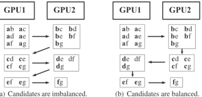
dis-(a) Candidates are imbalanced. (b) Candidates are balanced. Fig. 1 Prefix distribution of candidates.
tributes the candidates into GPUs according to their prefixes in Line 8. A na¨ıve way to distribute candidates is to as-sign prefixes to GPUs in round robin. However, this results in load imbalance among GPUs. For example, if there two GPUs and six 1-PFIs{a},{b},{c},{d},{e}, and{f}, then can-didate 2-itemsets can be assigned into GPUs as shown in Fig. 1(a). In this case, GPU 1 and GPU 2 handle 12 and 9 candidates, respectively. On the other hand, if the candidates are distributed as shown in Fig. 1(b), GPU 1 and GPU 2 deal with 11 and 10 candidates, respectively. The difference is small in this example, but it becomes more apparent as the numbers of prefixes and GPUs get larger. Thus we use the second way of prefix distribution.
At this point, GPUs have all the necessary data for pro-cessing: inclists, candidates, and probabilities. Each GPU extractsk-PFIs from the assigned candidates by using the single-GPU method in Line 11. The CPU gathers thek-PFIs from GPUs in Line 12. The collectedk-PFIs on the CPU are broadcasted to all the GPUs in Line 13, because thek -PFIs are necessary to do pruning in candidate generation. In Lines 14–15,kis incremented and GPUs generate candidate
k-itemsets from the (k−1)-PFIs extracted on each GPU. PD continues Lines 10–15 until no candidates are found.
PD minimizes data dependencies among GPUs by tributing candidates according to prefixes. However, the dis-tribution by prefix may result in load imbalance. This is be-cause the number of PFIs differs depending on a prefix. As a result, some GPUs may need to compute many SPMFs and other GPUs may compute a few SPMFs. Thus PD is not desirable from the viewpoint of load balancing.
3.1.2 Round-Robin Distribution
In this section, we explain a method that distributes candi-dates in a round-robin fashion. This method is called Round-Robin Distribution (RRD)due to its candidate-distribution scheme. While RRD has an almost identical algorithm to PD, major differences lie in the distribution and loop phases. In the distribution phase, candidates are allocated to GPUs in a round-robin fashion, instead of using prefixes.
In the loop phase, there are two modifications. The first modification is to generate candidates on the CPU rather than GPUs, thereby balancing loads of GPUs at each iter-ation. Although data transfer between CPU and GPUs oc-curs at each iteration, only candidates are transferred and the
communication time is negligible in practice.
The second modification is for inclusion check to em-ploy inclists of 1-itemsets rather than (k−1)-itemsets. In the case of PD, inclusion check of ak-itemsetXcan be per-formed with inclists of (k−1)-itemsets that are origins ofX, because Xand the origins reside in the same GPU. On the other hand, since RRD distributes candidates in round robin, it is probable that the two origins and their inclists reside in different GPUs. Hence, if a GPU tries to perform inclusion check with inclists of (k−1)-itemsets, the GPU may need to access inclists in another GPU. Consequently data trans-fer between GPUs, which should be avoided, occurs. To address this issue, we utilize the inclists of 1-itemsets that were already transferred in the initialization phase. In this case, inclusion check of ak-itemset is performed ask−1 bitwise AND operations among inclists ofk1-itemsets in-cluded inX.
3.1.3 Count-Based Distribution
We describe another candidate-distribution scheme called
Count-Based Distribution (CBD). CBD assigns candidates to GPUs by taking into account candidates’ cnt values. The rationale is that the cnt values determine the computing time of SPMFs [15], and the computing time of SPMFs domi-nates the processing time of candidates on GPUs. Therefore we can achieve load balancing if candidates are distributed by considering cnt values. To this end, we firstly need to estimate the computing times of SPMFs for particular cnt values.
We can estimate the computing time of an SPMF for a particular cnt value, if we know the computing time of an SPMF for the next-higher power of two of the cnt value. This is because the single-GPU method uses 2log2cnt(X)
transactions to compute the SPMF of an itemset X in or-der to simplify the computation on a GPU. In this work, we measure in advance the computing times of SPMFs for power-of-two numbers of transactions. Once the computing times are measured, this information can be used for any dataset, because the computing times are determined only by execution environments and are independent on datasets. To achieve load balancing, we also need to know the cnt values of candidates when assigning candidates to GPUs. If k = 1, the values are computed before the assignment. On the other hand, if k > 1, the cnt values are not computed at the assigning time, and thus need to be estimated. We here approximate cnt(X) as minX⊂X,|X|=k−1cnt(X). This value is an upper bound of the
actual cnt(X) value, and cnt(X) is expected to be less than this upper bound. Although the difference between the up-per bound and cnt(X) might become large, the difference is negligible in practice, because estimating a computing time requires only the next-higher power of two of cnt(X).
The algorithm of CBD is identical to RRD except for its candidate-distribution scheme. CBD distributes candi-dates to GPUs so that processing times on GPUs are as even as possible. The algorithm of candidate distribution firstly
Table 2 Characteristics of datasets.
Dataset Type Number of items Avg. size of transactions Number of transactions Density
Accidents real 468 33.8 340,183 7.2%
T25I10D500K synthetic 7558 25 499,960 0.33%
Kosarak real 41270 8.1 990,002 0.020%
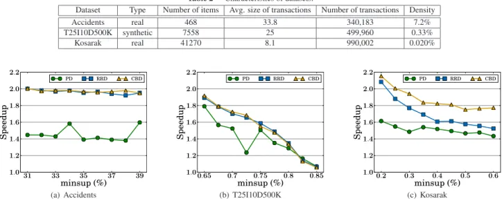
(a) Accidents (b) T25I10D500K (c) Kosarak
Fig. 2 Speedup of multi-GPU methods compared to the single GPU method on a single node.
initializes candidates and a processing time of each GPU to empty set and zero, respectively. Then the algorithm iterates the following two steps over candidates:
1. Find the GPU that has the minimum processing time. 2. Update candidates and processing time of the GPU. Having finished the distribution, CBD extracts PFIs on GPUs as in RRD.
3.2 A Method on a GPU Cluster
This section describes a method on a GPU cluster that is an extension of single-node methods described in Sect. 3.1. For the sake of simplicity, this paper assumes that all the nodes hold an input database.
The basic idea is identical to the single-node methods: Candidates are distributed among nodes and are processed in parallel. The detailed algorithm is as follows. First, each node extracts PFIs from candidates, which are evenly par-titioned among nodes. Each node processes distinct can-didates, and thus generates distinct PFIs. To generate next candidates, the PFIs extracted on a node need to be broad-casted to all other nodes.
Subsequently, candidate 2-itemsets are generated. Ei-ther RRD or CBD is used to determine which node pro-cesses specific candidates. The same candidate-distribution scheme is used to further distribute the candidates among GPUs within a node. Then, each node extracts 2-PFIs, and broadcasts the PFIs to other nodes. The above steps con-tinue with incrementingkby one until there is no candidate. Since only PFIs need to be communicated among nodes, the communication cost is very small and negligible.
4. Experiments
4.1 Experimental Setup
We implemented the proposed methods using CUDA [20],
OpenMP, and MPI. Experiments were conducted on a GPU cluster of eight nodes, each of which has two CPUs and two GPUs. The CPU is Intel Xeon E5645 with 6 cores running at 2.4 GHz. The GPU is NVIDIA Tesla M2090 with 512 cores running at 1.3 GHz. The nodes are connected via InfiniBand QDR (Quad Data Rate).
Table 2 summarizes the three datasets used in the ex-periments. The density of a dataset is computed as the average length of transactions divided by the number of items. Accidents and Kosarak are real datasets that are accessible on Frequent Itemset Mining Implementations (FIMI) Repository.†While Accidents is the densest dataset, Kosarak is the sparsest dataset. T25I10D500K is a synthetic dataset, generated by a data generator.†† The default val-ues of minsupon Accidents, T25I10D500K, and Kosarak are 33%, 0.65%, and 0.2%, respectively. Existential proba-bilities for the datasets are randomly drawn from a normal distribution with mean 0.5 and variance 0.02. The value of
minprobis fixed to 0.5 for all the experiments. 4.2 Results on a Single Node
This section evaluates the three methods on a single node (PD, RRD, and CBD). We first show the result of whole algorithms and then analyze the several aspects of the al-gorithms in detail. Figures 2(a)–2(c) show the speedups of the three methods compared to the single-GPU method [9], with varyingminsupvalues. We measured execution time as elapsed time from when the dataset is ready on CPU to when all the result are collected to CPU. Note that the com-munication time between CPU and GPU is included in the execution time. From the charts, we can make the following three observations:
1. The multi-GPU methods become increasingly faster
†http://fimi.cs.helsinki.fi/
††http://miles.cnuce.cnr.it/∼palmeri/datam/DCI/
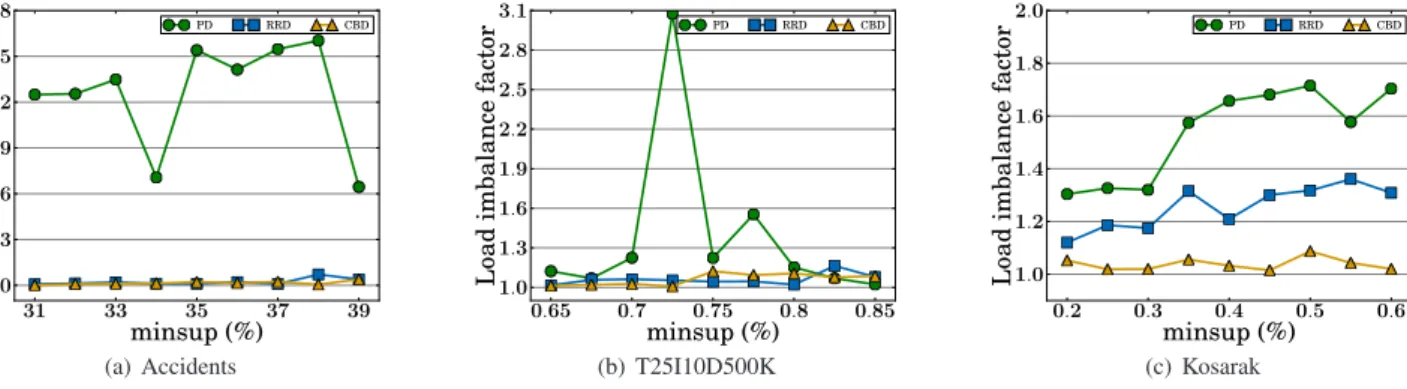
(a) Accidents (b) T25I10D500K (c) Kosarak Fig. 3 Load imbalance factors between two GPUs.
than the single-GPU method, as theminsupvalue de-creases.
2. RRD and CBD are generally faster than PD.
3. CBD outperforms RRD on Kosarak, while CBD and RRD exhibit similar performance on Accidents and T25I10D500K.
The first observation is due to the fact that small
minsupvalues make the number of candidates large, and thus GPUs have much more workload to be done in parallel. Although the number of candidates is small on Accidents, Fig. 2(a) shows near-linear speedups. This is because the cnt values become very large (nearly 250,000) on Accidents, and hence the computation of SPMFs on Accidents is far more computationally demanding than the computation on T25I10D500K and Kosarak. As a result, the overall process-ing time on GPUs is dominated by the time of computprocess-ing SPMFs, which can be performed in parallel. Note that the RRD and CBD on Kosarak achieve super-linear speedups as shown in Fig. 2(c). This is because candidate generation on a CPU is faster than that on GPUs if the number of generated candidates becomes very large.
The second observation results from the load imbal-ance in PD. To verify this observation, we use aload im-balance factordefined as the ratio of the longest processing time of GPUs to the shortest processing time of GPUs. The factor takes the value of 1 if the load is completely balanced, and the factor increases as the load is more imbalanced. Fig-ures 3(a)–3(c) show the load imbalance factors between two GPUs as a function ofminsupvalue. These charts reveal that RRD and CBD achieve better load balancing than PD on all the datasets. The jags of PD in Figs. 2(a) and 2(b) are due to the skewness in the numbers of PFIs with diff er-ent prefixes. If one GPU processes candidates with prefixes that generate many PFIs, the other GPU generates few PFIs. Consequently the load imbalance occurs.
The third observation emerges from a characteristic of datasets and the better capability of CBD for load balancing. The characteristic is related to the dispersion of cnt values. For instance, candidates in Kosarak have a wide range of cnt values (2,000–600,000). Since CBD distributes candidates by taking into account cnt values, CBD accommodates to such variability, unlike RRD, which statically assigns
can-didates to GPUs. As a result, CBD achieves better load balancing than RRD, and realizes higher speedup ratios, as shown in Figs. 2(c) and 3(c). On the other hand, CBD and RRD on Accidents and T25I10D500K exhibit similar per-formance as shown in Figs. 2(a) and 2(b). This is because the cnt values (i.e., processing times) of candidates in Ac-cidents and T25I10D500K do not vary much. Thus it is sufficient to distribute candidates in round robin in order to achieve load balancing.
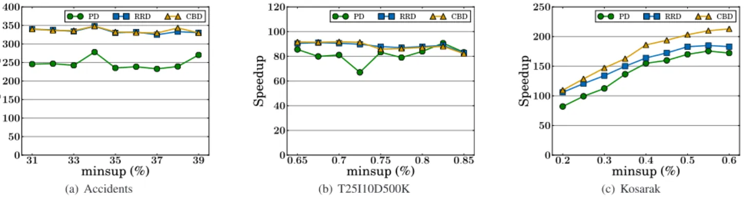
As a summary of this section, we demonstrate how fast our methods run compared to the serial execution on CPU. Figures 4(a)–4(c) shows the speedup values. On Ac-cidents, RRD and CBD achieve the speedup of about 350; on t25i10d500k, they are 90 times faster. The results on these two datasets exhibit stable speedup with respect to
minsupvalues. On the other hand, the speedup on Kosarak decreases as making theminsupvalue smaller. This is be-cause when aminsupvalue is small, the number of candi-dates with small cnt values increases and more time is spent for the filtering step.
4.2.1 Time Breakdown at Each Iteration
This section further analyzes the most efficient method, CBD, to clarify influences of each step of the algorithm on overall execution time. Figures 5(a)–5(c) show the execu-tion time of five steps at each iteraexecu-tion. The five steps con-sists of candidate generation, inclusion check, pruning, fil-tering, and computing SPMFs. The time of pruning atk=1 is not shown because it is contained in inclusion check.
The most influential step is computing SPMFs on all the three datasets. On Accidents, this step takes 90% of overall execution time. When using T25I10D500K and Kosarak, CBD spends about 60% of overall time. On these datasets, more time is spent at inclusion check and pruning compared to the case of Accidents. This is due to the larger number of candidates and the larger sizes of datasets. 4.2.2 Larger Memory Footprint
In this section, we make memory footprint on GPU larger by loweringminsup values on Kosarak, to see the advan-tage of larger memory space with multiple GPUs. Figure 6
(a) Accidents (b) T25I10D500K (c) Kosarak Fig. 4 Speedup of multi-GPU methods compared to the serial execution on CPU.
(a) Accidents (b) T25I10D500K (c) Kosarak
Fig. 5 Execution time breakdown of CBD at each iteration.
Fig. 6 Execution time on Kosarak with smallminsupvalues.
depicts the execution time of single-GPU method, RRD, and CBD. Some points of the single-GPU method are not shown because it does not work due to running out of memory. Ta-ble 3 shows the sizes of inclists, which are the largest data on GPUs.
The single-GPU method works only when theminsup
value is greater or equal to 0.18 %. This result and Table 3 indicate that the single-GPU method can deal with inclists of 3.6 GB but cannot deal with inclists of 4.1 GB. On the other hand, RRD and CBD work with the cases of smaller
minsupvalues. Since RRD and CBD uses two GPUs, they can handle inclists of 7.0 GB (minsup = 0.14), which is about 2 times of 3.6 GB. However, RRD and CBD are also running out of memory whenminsup=0.13. In this case, the size of inclists is 8.6 GB, which is more than two times of 4.1 GB.
Table 3 The sizes of inclists on GPU with varyingminsupvalues. minsup(%) 0.13 0.14 0.15 0.16 0.17 0.18 0.19 Inclist size (GB) 8.6 7.0 5.5 4.7 4.1 3.6 3.0
4.2.3 CPU–GPU Communication Time
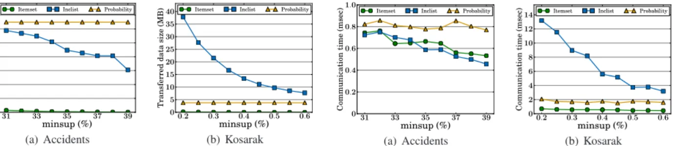
This section evaluates the transferred data size and commu-nication time between CPU and GPU. Figures 7(a) and 7(b) show the sizes of transferred data between CPU and GPU on Accidents and Kosarak, respectively.Itemsetin the fig-ures include candidates and PFIs. We show only the result of CBD because other methods show similar results. In ad-dition, we omit the result on T25I10D500K because it is similar to the result of Kosarak.
On Accidents, the array of probabilities is the largest transferred data and itemsets are the smallest data. Inclists lie in the middle of these two data. On the other hand, in-clists become the largest transferred data on Kosarak. This is because the number of 1-PFIs on Kosarak, which corre-sponds to the number of inclists, is much larger than the number of 1-PFIs on Accidents.
Figures 8(a) and 8(b) illustrate communication time be-tween CPU and GPU on Accidents and Kosarak, respec-tively. In general, it can be seen from the figures that the communication time is proportional to the data size. One ex-ception isItemseton Accidents; the communication takes almost the same time as inclists, although itemsets are small. This is because itemsets are communicated multiple times,
(a) Accidents (b) Kosarak Fig. 7 Transferred data size between CPU and GPU.
(a) Accidents (b) Kosarak
Fig. 8 Communication time between CPU and GPU.
(a) Accidents (b) T25I10D500K (c) Kosarak
Fig. 9 The breakdown of execution time on the GPU cluster of eight nodes.
(a) Accidents (b) T25I10D500K (c) Kosarak
Fig. 10 Load imbalance factors among all the GPUs on the GPU cluster.
while the inclists are transferred only once. 4.3 Results on the GPU Cluster
This section evaluates two variants of the method on the GPU cluster with two candidate-distribution schemes, namely RRD and CBD. Figures 9(a)–9(c) show executions times of RRD and CBD and their breakdowns with vary-ing number of nodes and the default values of minsup. Load imbalance factors among all GPUs are also shown in Figs. 10(a)–10(c). We measured execution time as elapsed time between when all nodes finish loading data and when a master node collects all PFIs. The execution time consists of three parts: communication time among nodes (Comm), execution time on GPU (GPU), and execution time on CPU (CPU). More specifically,GPUcomprises inclusion check for
k>1, pruning fork >1, filtering, and computing SPMFs.
CPUincludes inclusion check and pruning fork=1,
candi-date generation, and data transfer between CPU and GPU. As mentioned in Sect. 3.2, we assume that all the nodes have the complete dataset. Thus the dataset does not need to be communicated among the nodes.
On Accidents, Figs. 9(a) and 10(a) show that CBD achieves slightly better load balancing than RRD and a 7.1 times speedup on eight nodes. Since the computation of SPMFs on Accidents is computationally expensive as men-tioned in Sect. 4.2, GPUs can have much work processed in parallel. Thus, CBD and RRD show high scalability.
Figure 9(b) shows that CBD and RRD result in the al-most same performance on T25I10D500K, and the speedup on eight nodes is 4.5. The methods on this dataset do not achieve high scalability as in the case of Accidents. This is because cnt values on T25I10D500K are small, and there is little work processed by GPUs. Thus the execution time on CPU, which is incurred by all nodes, dominates 10–25% of overall execution time, and becomes a bottleneck.
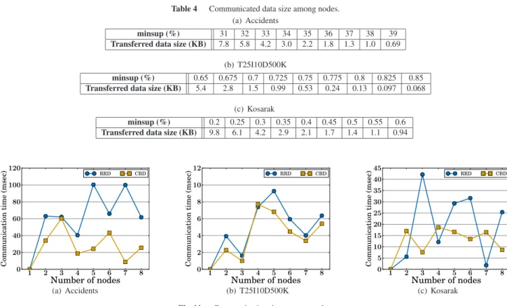
Mean-Table 4 Communicated data size among nodes. (a) Accidents
minsup (%) 31 32 33 34 35 36 37 38 39 Transferred data size (KB) 7.8 5.8 4.2 3.0 2.2 1.8 1.3 1.0 0.69
(b) T25I10D500K
minsup (%) 0.65 0.675 0.7 0.725 0.75 0.775 0.8 0.825 0.85 Transferred data size (KB) 5.4 2.8 1.5 0.99 0.53 0.24 0.13 0.097 0.068
(c) Kosarak
minsup (%) 0.2 0.25 0.3 0.35 0.4 0.45 0.5 0.55 0.6 Transferred data size (KB) 9.8 6.1 4.2 2.9 2.1 1.7 1.4 1.1 0.94
(a) Accidents (b) T25I10D500K (c) Kosarak
Fig. 11 Communication time among nodes.
while, the fact that CBD and RRD have similar performance is due to the little variability of cnt values on T25I10D500K, as discussed in Sect. 4.2.
On Kosarak, CBD achieves much better load balanc-ing than RRD (Fig. 10(c)), and shows a 4.9 times speedup on eight nodes. Since candidates have a wide range of cnt values on this dataset, RRD cannot balance the load among nodes, while CBD accommodates to the variability. On av-erage, CBD is 1.3 times faster than RRD on this dataset.
Figure 11 focuses on the communication time among nodes. Table 4 summarizes the sizes of communicated data among nodes. Since the proposed methods only commu-nicate PFIs, their sizes are very small and not so different among datasets (Table 4). However, the communication time can vary largely. For example, the communication on Accidents takes 10 times longer than the communication on T25I10D500K (Figs. 11(a) and 11(b)). This is because the communication time include the synchronization time. In other words, each node needs to wait until all the nodes fin-ish to find PFIs. That is why the communication takes much longer on Accidents, where the computation of SPMFs is very expensive. For the same reason, on average, the com-munication of CBD is shorter than that of RRD.
5. Related Work
This section reviews related work on frequent itemset min-ing and probabilistic frequent itemset minmin-ing.
Frequent itemset mining.The problem of association rule mining was firstly introduced by Agrawal et al. [3].
As-sociation rule mining consists of two steps: frequent itemset mining and finding association rules. Since frequent itemset mining is more computationally intensive, many algorithms have been proposed to accelerate the mining. Among the algorithms, there are two major algorithms, namely Apri-ori [4] and FP-growth [8].
Parallelization of these algorithms has been widely studied. In the late 1990s, distributed-memory systems were mainly used as the underlying architecture. Zaki summa-rized such algorithms [19]. More recently, Li et al. [10] de-signed a parallel algorithm of FP-growth on a massive com-puting environment using MapReduce. ¨Ozkural et al. [13] introduced a data distribution scheme based on a graph-theoretic approach.
Frequent itemset mining on GPUs has been also stud-ied [5], [7], [14], [16]. Fang et al. [7] proposed two ap-proaches, GPU-based and CPU-GPU hybrid methods. The GPU-based method utilizes bitstrings and bit operations for fast support counting, running entirely on a GPU. The hy-brid method adopts the trie structure on a CPU and counts supports on a GPU. Teodoro et al. [16] parallelized the Tree Projection algorithm [1] on a GPU as well as a multi-core CPU. Amossen et al. [5] presented a novel data layout
BatMapto represent bitstrings. This layout is well suited to parallel processing and compact even for sparse data. Then they make use of BatMap to accelerate frequent itemset min-ing. Silvestri et al. [14] proposed a GPU version of a state-of-the-art algorithmDCI[11].
Probabilistic frequent itemset mining. While the above-mentioned parallel algorithms work well for the
con-ventional certain transaction databases, they cannot ef-fectively process frequent itemset mining from uncertain databases, which gains increasing importance in order to handle data uncertainty. There is much work for modeling, querying, and mining such uncertain data (see a survey by Aggarwal and Yu [2] for details and more information).
To mine frequent itemsets with taking into account the uncertainty, a number of algorithms have been proposed. Bernecker et al. [6] proposed an algorithm to find probabilis-tic frequent itemsets under the attribute-uncertainty model, where existential probabilities are associated with items. On the other hand, Sun et al. [15] considered the tuple-uncertainty model, where existential probabilities are asso-ciated with transactions. Recently, Tong et al. [17] imple-mented existing representative algorithms and test their per-formance with uniform measures fairly.
Several attempts to accelerate these algorithms also ex-ist. Wang et al. [18] developed an algorithm to approximate the probability that determines whether itemsets are PFIs or not. Our previous work [9] presented an algorithm using a single GPU based on the work by Sun et al. [15]. We have extended this method to use multiple GPUs in this paper.
6. Conclusions
This paper has proposed methods of probabilistic frequent itemset mining using multiple GPUs. The methods run in parallel by distributing candidates among GPUs. The pro-posed method PD assigns candidates to GPUs according to their prefixes. Then we have described RRD and CBD, which take into consideration load balancing. RRD dis-tributes candidates to GPUs in a round-robin fashion, while CBD uses the cnt values of candidates to achieve better load balancing. We have also presented methods on a GPU clus-ter by extending RRD and CBD. Experiments on a single node showed that CBD achieves the best load balancing and results in the fastest algorithm. Experiments on a GPU clus-ter of eight nodes revealed that our proposed methods are effective if there is sufficient workload to be processed on GPUs. Future work involves developing a CPU-GPU hy-brid method that utilizes CPUs and GPUs simultaneously. In addition, more sophisticated multi-node methods should be considered.
Acknowledgments
This work was supported by JSPS KAKENHI Grant Num-ber 24240015 and HA-PACS Project for advanced interdis-ciplinary computational sciences by exa-scale computing technology.
References
[1] R.C. Agarwal, C.C. Aggarwal, and V.V.V. Prasad, “A tree projection algorithm for generation of frequent item sets,” J. Parallel Distrib. Comput., vol.61, no.3, pp.350–371, March 2001.
[2] C.C. Aggarwal and P.S. Yu, “A survey of uncertain data algorithms and applications,” IEEE Trans. Knowl. Data Eng., vol.21, no.5,
pp.609–623, May 2009.
[3] R. Agrawal, T. Imieli´nski, and A. Swami, “Mining association rules between sets of items in large databases,” Proc. ACM SIGMOD Int’l Conf. Management of Data (SIGMOD), pp.207–216, 1993. [4] R. Agrawal and R. Srikant, “Fast algorithms for mining
associa-tion rules,” Proc. 20th Int’l Conf. Very Large Data Bases (VLDB), pp.487–499, 1994.
[5] R.R. Amossen and R. Pagh, “A new data layout for set intersection on GPUs,” Proc. IEEE Int’l Parallel & Distributed Processing Symp. (IPDPS), pp.698–708, 2011.
[6] T. Bernecker, H.-P. Kriegel, M. Renz, F. Verhein, and A. Zuefle, “Probabilistic frequent itemset mining in uncertain databases,” Proc. 15th ACM SIGKDD Int’l Conf. Knowledge Discovery and Data Mining (KDD), pp.119–128, 2009.
[7] W. Fang, M. Lu, X. Xiao, B. He, and Q. Luo, “Frequent itemset mining on graphics processors,” Proc. Fifth Int’l Workshop on Data Management on New Hardware (DaMoN), pp.34–42, 2009. [8] J. Han, J. Pei, and Y. Yin, “Mining frequent patterns without
candi-date generation,” Proc. ACM SIGMOD Int’l Conf. Management of Data (SIGMOD), pp.1–12, 2000.
[9] Y. Kozawa, T. Amagasa, and H. Kitagawa, “GPU acceleration of probabilistic frequent itemset mining from uncertain databases,” Proc. 21st Int’l Conf. Information and Knowledge Management (CIKM), pp.892–901, 2012.
[10] H. Li, Y. Wang, D. Zhang, M. Zhang, and E.Y. Chang, “PFP: Par-allel FP-growth for query recommendation,” Proc. ACM Conf. Rec-ommender Systems (RecSys), pp.107–114, 2008.
[11] S. Orlando, P. Palmerini, R. Perego, and F. Silvestri, “Adaptive and resource-aware mining of frequent sets,” Proc. IEEE Int’l Conf. Data Mining (ICDM), pp.338–345, 2002.
[12] J.D. Owens, M. Houston, D. Luebke, S. Green, J.E. Stone, and J.C. Phillips, “GPU computing,” Proc. IEEE, vol.96, no.5, pp.879–899, May 2008.
[13] E. Ozkural, B. Ucar, and C. Aykanat, “Parallel frequent item set mining with selective item replication,” IEEE Trans. Parallel Distrib. Syst., vol.22, no.10, pp.1632–1640, Oct. 2011.
[14] C. Silvestri and S. Orlando, “gpuDCI: Exploiting GPUs in frequent itemset mining,” Proc. 20th Euromicro Int’l Conf. Parallel, Dis-tributed and Network-based Processing (PDP), pp.416–425, 2012. [15] L. Sun, R. Cheng, D.W. Cheung, and J. Cheng, “Mining uncertain
data with probabilistic guarantees,” Proc. 16th ACM SIGKDD Int’l Conf. Knowledge Discovery and Data Mining (KDD), pp.273–282, 2010.
[16] G. Teodoro, N. Mariano, W. Meira, Jr., and R. Ferreira, “Tree Projection-based Frequent Itemset Mining on Multicore CPUs and GPUs,” Proc. 22nd Int’l Symp. Computer Architecture and High Performance Computing (SBAC-PAD), pp.47–54, 2010.
[17] Y. Tong, L. Chen, Y. Cheng, and P.S. Yu, “Mining frequent item-sets over uncertain databases,” Proc. VLDB Endow., vol.5, no.11, pp.1650–1661, July 2012.
[18] L. Wang, D.W. Cheung, R. Cheng, S.D. Lee, and X.S. Yang, “Ef-ficient mining of frequent item sets on large uncertain databases,” IEEE Trans. Knowl. Data Eng., vol.24, no.12, pp.2170–2183, Dec. 2012.
[19] M.J. Zaki, “Parallel and distributed association mining: A survey,” IEEE Concurrency, vol.7, no.4, pp.14–25, Oct. 1999.
Yusuke Kozawa received the B.Sc. and M.Eng. degrees from University of Tsukuba, Japan, in 2011 and 2013, respectively. He is currently a Ph.D. student at Graduate School of Systems and Information Engineering, Univer-sity of Tsukuba. His research interests include databases, data mining, and parallel computing.
Toshiyuki Amagasa received B.E., M.E., and Ph.D degrees from the Department of Com-puter Science, Gunma University in 1994, 1996, and 1999, respectively. Currently, he is an as-sociate professor at the Division of Information Engineering, Faculty of Engineering, Informa-tion and Systems, University of Tsukuba. His research interests cover database systems, data mining, and database application in scientific domains. He is a senior member of IEICE and IEEE, and a member of DBSJ, IPSJ, and ACM.
Hiroyuki Kitagawa received the B.Sc. gree in physics and the M.Sc. and Dr.Sc. de-grees in computer science, all from the Univer-sity of Tokyo, in 1978, 1980, and 1987, respec-tively. He is currently a full professor at Faculty of Engineering, Information and Systems and at Center for Computational Sciences, Univer-sity of Tsukuba. His research interests include databases, data integration, data mining, stream processing, information retrieval, and scientific databases. He is Vice President of DBSJ and a Fellow of IPSJ and IEICE. He is a member of ACM, IEEE Computer So-ciety, and JSSST.