Semiparametric efficiency bound for models of sequential moment restrictions containing unknown functions

Semiparametric efficiency

bound for models of

sequential moment

restrictions containing

unknown functions

Chunrong Ai

Xiaohong Chen

The Institute for Fiscal Studies

Department of Economics, UCL

Semiparametric E¢ ciency Bound for Models of Sequential

Moment Restrictions Containing Unknown Functions

Chunrong Ai

Xiaohong Chen

First draft: September 2004, Revised version: September 2009

Abstract

This paper computes the semiparametric e¢ ciency bound for …nite dimensional parame-ters identi…ed by models of sequential moment restrictions containing unknown functions. Our results extend those of Chamberlain (1992b) and Ai and Chen (2003) for semiparametric con-ditional moment restriction models with identical information sets to the case of nested infor-mation sets, and those of Chamberlain (1992a) and Brown and Newey (1998) for models of sequential moment restrictions without unknown functions to cases with unknown functions of possibly endogenous variables. Our bound results are applicable to semiparametric panel data models and semiparametric two stage plug-in problems. As an example, we compute the e¢ ciency bound for a weighted average derivative of a nonparametric instrumental variables (IV) regression, and …nd that the simple plug-in estimator is not e¢ cient. Finally, we present

Chen is grateful to Lars Peter Hansen for numerous insightful comments about e¢ ciency of GMM and related models and methods. We are grateful to Jim Powell for his encouragement upon hearing the …rst presentation in 2005. We thank Demian Pouzo for the Monte Carlo study, and Jinyong Hahn, Alex Torgovitsky, the guest coeditor, three anonymous referees for suggestions that improve the exposition. We also thank D. Andrews, D. Bhattacharya, R. Blundell, J. Horowitz, W. Newey, E. Tamer, and participants of 2005 World Congress Econometric Society Meetings, 2007 LSE Conference in honor of Peter Robinson, 2007 CIRANO and CIREQ econometric conference on GMM in Montreal, econometric workshops at various universities for helpful comments. Ai’s research is supported by 2003 summer grant from the Warrington Business School at University of Florida and Project 211 Phase III and Shanghai Leading Academic Discipline Project (Number: B803) at Shanghai University of Finance and Economics, China. Chen’s research is supported by the National Science Foundation grants SES-0318091 and SES-0631613. All errors are the responsibility of the authors.

y_{Department of Economics, University of Florida, Gainesville, FL 32611, USA, and Shanghai University of Finance}

and Economics, China. Email: [email protected]‡.edu.

z_{Corresponding author. Xiaohong Chen, Cowles Foundation for Research in Economics, Yale University, Box}

an optimally weighted, orthogonalized, sieve minimum distance estimator that achieves the semiparametric e¢ ciency bound.

JEL Classi…cation: C14; C22

Keywords: Sequential moment models; Semiparametric e¢ ciency bounds; Optimally weighted orthogonalized sieve minimum distance; Nonparametric IV regression; Weighted average deriv-atives; Partially linear quantile IV

1

Introduction

Since the publication of Hansen’s (1982) seminal work on the Generalized Method of Moments (GMM), moment restriction models have become a popular and useful framework for analyzing eco-nomic data. See Hansen (2007) for an excellent review of the original GMM, its numerous extensions and a wide range of applications.

Motivated by an ever expanding variety of applications, one important branch of extensions fo-cuses on semiparametric e¢ ciency bounds and e¢ cient estimation of more general moment restriction models.1 _{In this paper, we contribute to this line of research by characterizing the semiparametric}

e¢ ciency bound for …nite dimensional parameters ( o) that are identi…ed by models of sequential

moment restrictions containing unknown functions:

E[ _t(Z; o; ho( ))jX(t)] = 0 for t = 1; :::; T almost surely, (1)

where Z = (Y0_{; X}0₎0 _{denotes a multivariate random variable with support Z and X X}(T)_{, and}

t(z; ; h( )) denotes a d t 1 vector of residual functions whose functional forms are known up to

the unknown true parameter values ( o; ho), with ho( ) = (ho1( ); :::; hoq( )) as the q 1 vector of

real-valued measurable functions that may depend on endogenous variables Y and other unknown parameters. E[_jX(t)_{]denotes the conditional expectation under the true (but unknown) conditional}

distribution function F_ZjX(t) for t = 1; :::; T. The sigma-…eld generated by the conditioning variable 1_{See, for example, Hansen (1985, 1993), Hansen, Heaton and Ogaki (1988), Chamberlain (1987, 1992a, 1992b),}

Newey (1993, 2004), Hahn (1997), Carrasco and Florens (2000), Ai and Chen (2003), Chernozhukov and Hong (2003), Donald, Imbens and Newey (2003), Kitamura, Tripathi and Ahn (2004), Newey and Smith (2004), Antoine, Bonnal and Renault (2007),to name only a few.

X(t)_{, X}(t) _{, satis…es a nesting structure}2

f1_g X(1) X(2) X(T) .

When X(1) is the constant 1, the conditional expectation E[ ₁(Z; ; h( ))_jX(1)] is simply the uncon-ditional expectation E[ ₁(Z; ; h( ))]. Thus model (1) includes unconditional moment restrictions as a special case.

Model (1) includes many existing econometric models. First, it includes semiparametric and nonparametric panel data models where the information set expands over time. Second, it nests widely used semiparametric models that are estimated via two-stage plug-in procedures. For example, with T = 2; = ( 0₁; 0₂)0, X(1) = 1 and X =X(2), model (1) becomes the following semiparametric “plug-in” problem:

E[ ₁(Z; o1; o2; ho( ))] = 0with dim( 1) = dim( 1); (2)

E[ ₂(Z; o2; ho( ))jX(2)] = 0; (3)

where the unknown parameter o2 and the unknown function ho( ) can be estimated using the

con-ditional moment restriction (3), and can then be plugged into the unconcon-ditional moment restriction (2) to compute the parameter o1. An example of the plug-in problem is the estimation of a weighted

average derivative of a possibly nonlinear nonparametric instrumental variables (IV) model:

o =E[W(Y2)rho(Y2)]; E[ 2(Z;ho(Y2))jX(2)] = 0;

where W()is a known positive weight function and_rho()denotes the …rst derivative ofho. Leading

examples of the functional forms of ₂(Z;h(Y2))include 2(Z;h(Y2)) =Y1 h(Y2) for nonparametric

mean IV regression and ₂(Z;h(Y2)) = 1fY1 h(Y2)g 0:5 for nonparametric median IV

regres-sion. Note that our model (1) allows for more general plug-in problems where the unconditional moment restrictionE[ ₁(Z; o1; o2; ho( ))] = 0is overidenti…ed for o1 (ordim( 1)>dim( 1)). Many

semiparametric program evaluation models, semiparametric missing data models, choice-based sam-pling problems, some recent nonclassical measurement error models and some semiparametric control function models could also …t into framework (1).

2_{This sequential restriction on the sigma-…elds allows us to gather all moment restrictions using the same set of}

WhenT = 1 and X(1) _{=X, model (1) becomes the semiparametric conditional moment}

restric-tion model with the same condirestric-tioning informarestric-tion set: E[ (Z; o; ho( ))jX] = 0.3 For this model,

Chamberlain (1992b), Ai and Chen (2003) and Chen and Pouzo (2009) characterized the semipara-metric e¢ ciency bound of o; and Ai and Chen (2003), Otsu (2008) and Chen and Pouzo (2009)

considered e¢ cient estimation of o. However, these e¢ ciency bound and e¢ cient estimation results

do not cover semiparametric models with sequential information sets like (1).

Without unknown functions ho( ), model (1) becomes the one studied by Chamberlain (1992a),

Hahn (1997) and Brown and Newey (1998). In particular, under the assumption that o is identi…ed

by the model E[ _t(Z; o)jX(t)] = 0, t = 1; :::; T; where f1g X(1) X(T) ,

Chamberlain (1992a) established the semiparametric e¢ ciency bound and Hahn (1997) obtained an e¢ cient estimator of o. Brown and Newey (1998) studied the semiparametric e¢ ciency bound and

suggested some e¢ cient estimators of parameters that are de…ned as unconditional expectations; one of their models is o1 =E[g(Z; o2)]; E[ 2(Z; o2)jX(2)] = 0 with known functional forms of g and 2.

In this paper we extend their results to the general model (1) that contains unknown functions ho( )

which may depend on endogenous variables.

Ai and Chen (2007) studied consistent estimation of ( o; ho) identi…ed by the general model (1)

with T 2, and established the root-n asymptotic normality of their estimator of o. But, to the

best of our knowledge, there is no published work on the semiparametric e¢ ciency bound or e¢ cient estimation of o for model (1), not even for the important special case of the semiparametric

plug-in problem (2)-(3) when ho( )is an unknown function of endogenous variables. There are e¢ ciency

results for various special cases of the model (1) when the unknown functionho( )does not depend on

endogenous variables. For example, Newey and Stoker (1993) computed the semiparametric e¢ ciency bound and presented an e¢ cient estimator for the weighted average derivative when the unknown

ho( ) is a measurable function of conditioning variables (say X(2) in terms of our notation) only.

Our plug-in problem (2)-(3) extends their setup to allow for ho( ) to be a function of endogenous

variables. Since many economic structural models satisfy the sequential moment restrictions (1) with

ho( ) being an unknown function ofY, our extension is a useful one.

A key step in our calculation of the semiparametric e¢ ciency bound for the general model (1) is to sequentially orthogonalize the residual functions t(Z; o; ho( )) for t= 1; :::; T. The semiparametric

e¢ ciency bound is then obtained by optimally weighting the orthogonalized residual functions. When

3_{See Newey and Powell (2003), Chernozhukov, Imbens and Newey (2007), and Chen and Pouzo (2008a) for}

specialized to the models considered by Chamberlain (1987, 1992a, b), Brown and Newey (1998), Ai and Chen (2003) and Chen and Pouzo (2009), our semiparametric e¢ ciency bound coincides with the bounds derived by these authors for their respective models. Although the e¢ ciency bounds do not have explicit closed form expressions for general conditional moment models involving several unknown functions with di¤erent arguments, these bounds can be computed analytically for many speci…c sequential moment models containing only one unknown function. Our characterization of the e¢ ciency bound is useful in evaluating and comparing di¤erent estimators for the general model (1). It also sheds lights on how to construct new estimators that attain the e¢ ciency bound for o.

Speci…cally, it clearly suggests that any e¢ cient estimation procedure has to account for both the correlation between the residual functions _t(Z; o; ho( )) as well as their conditional

heteroskedas-ticity. For model (1) with nonsingular e¢ ciency bound for o, we provide an optimally weighted,

orthogonalized, sieve minimum distance (SMD) estimator that is root-n asymptotically e¢ cient for

o.

When applied to the semiparametric plug-in problem (2)-(3), our e¢ ciency bound result reveals that one just needs to use the conditional moment model E[ ₂(Z; o2; ho( ))jX(2)] = 0 alone to

construct an e¢ cient estimator of o2. However, any e¢ cient estimator of o1 has to account for the

correlation between the two residuals ₁(Z; o1; o2; ho( )) and 2(Z; o2; ho( )) conditional on X(2).

In particular, whenever E[ ₁(Z; o1; o2; ho( )) 2(Z; o2; ho( ))jX(2)]6= 0, any simple plug-in estimator b₁, de…ned as a solution to 1_n

n P

i=1 1

(Zi;b1;b2;bh( )) = 0, is not e¢ cient for o1, regardless of how one

computes the …rst stage estimator(b2;bh( )). For example, to estimate the weighted average derivative

o1 =E[W(Y2)rho(Y2)]of a NPIV regressionE[Y1 ho(Y2)jX(2)] = 0, Ai and Chen (2007) presented

a simple plug-in estimatorb1 = 1_n

n P i=1

W(Y2i)rbh(Y2i)wherebh( )is a SMD estimator ofho, and derived

the root-n asymptotic normality of this estimatorb1. To compute a simple plug-in estimator of o1,

instead of using their SMD estimator of ho, one could use other existing NPIV estimators, such as

the estimators of Hall and Horowitz (2005), Darolles, Florens and Renault (2002), Blundell, Chen and Kristensen (2007). Unfortunately, since E[W(Y2)rho(Y2)fY1 ho(Y2)gjX(2)]6= 0, none of these

simple plug-in estimators attain the semiparametric e¢ ciency bound for o1.

The rest of the paper is organized as follows: Section 2 …rst computes the semiparametric e¢ ciency bound for o in the general model (1), and then applies the bound result to the plug-in problem

(2)-(3). Section 3 applies the e¢ ciency bound result to several non-trivial examples, including estimating the weighted average derivative of ho(Y2) in the NPIV regression E[Y1 ho(Y2)jX(2)] = 0 or in the

…rst discusses semiparametric e¢ cient estimation of o for the general model (1) and then presents a

small Monte Carlo study to compare the ine¢ cient simple plug-in estimator versus several e¢ cient estimators of the average derivative of a NPIV regression. Section 5 concludes with suggestions of other e¢ cient estimation procedures. All proofs are contained in the appendix.

2

Semiparametric E¢ ciency Bound

We begin by computing the semiparametric e¢ ciency bound of o. Our calculation of the bound

closely follows the approach of Stein (1956), Newey (1990), Chamberlain (1992a, b) and others (see the appendix for details). We …rst sequentially orthogonalize the original sets of residual functions

t(Z; o; ho( )) for t= 1; :::; T. This procedure is called forward …ltering by Hayashi and Sims (1983)

in their study of linear time series rational expectation models, and has been used in Hansen, Heaton and Ogaki (1988), Chamberlain (1992a) and others in time series and panel data models without an unknown functionho( ). In the following we denote Rd as an open, …nite-dimensional parameter

space with o2 . Let(H;jj jjH)denote an in…nite-dimensional metric space withH=H1 Hq

and ho = (ho1; :::; hoq)2 H, where ho1,..., hoq are real-valued measurable functions. Let A = H

and o = ( 0o; ho)2 A. For any = ( 0; h)2 A, we de…ne

"T(Z; ) T(Z; ); "s(Z; ) s(Z; ) T X t=s+1 s;t(X(t))"t(Z; ) for s=T 1; :::;1; where s;t(X(t)) E[ s(Z; o)"t(Z; o)0jX(t)]f ot(X(t))g 1 for s < t and ot(X(t)) E["t(Z; o)"t(Z; o)0jX(t)]:

For any = ( 0; h)_{2 A}, we denote

ms(X(s); ) Ef"s(Z; )jX(s)g for s= 1; :::; T:

We note that by construction

and

E["s(Z; o)"t(Z; o)0jX(t)] = 0 for any s < t:

This implies that

E_f"s(Z; o)"t(Z; o)v(X(s))q(X(t))g= 0 for any s6=t and any measurable functions v and q.

Also, "s(Z; ) = s(Z; ) (or s;t(X(t)) = 0 for all s < t) if s(Z; o) is measurable with respect to

the sigma …eld generated by X(s+1)_{. Throughout the paper we assume the following conditions hold:}

Assumption 1: (i) The data_fZi = (Yi0; Xi0)0gni=1 is a random sample from an unknown distribution

of Z on_Z; (ii) o = ( 0o; ho)2 A satis…es model (1).

Let _f ( ) = ( ( ); h( )) : 0 1_{g A} be an arbitrarily smooth path in satisfying (0) = o,

(1) = , d_d( )_j =0 = o, and dh_d( )j =0 =h ho h. Assumption 2: For t= 1; :::; T, dmt(X(t); ( ))

d j =0 is well-de…ned and has …nite second moment.

Fort = 1; :::; T denote dmt(X(t); o) d [ o] = dE_f"t(Z; ( ))jX(t)g d j =0 = dmt(X(t); o) d 0 ( o) + dmt(X(t); o) dh [h ho] where dmt(X(t); o) d = dE_f"t(Z; ; ho)jX(t)g d j = o, dmt(X(t); o) dh [h ho] = dE_f"t(Z; o; h( ))jX(t)g d j =0:

Assumption 3: For all t = 1; :::; T, (i) ot(X(t)) is non-singular with probability one and (ii)

E h dmt(X(t); o) d0 i0 ot(X(t)) 1 h dmt(X(t); o) d 0 i <₁. For any h_{2 H}, de…ne a pseudo-metric _jjh hojj as

jjh hojj2 T X t=1 E _fdmt(X (t)_; o) dh [h ho]g 0 ot(X(t)) 1f dmt(X(t); o) dh [h ho]g : (4)

x. For each component j (of ), j = 1; :::; d , let r_oj _{2 W} denote one solution to inf rj_2W T X t=1 E ( f ot(X(t))g 1 2 dmt(X (t)_; o) d j dmt(X(t); o) dh [r j_] 2 e ) ; (5)

which solves: for all rj _{2 W},

T X t=1 E ( dmt(X(t); o) d j dmt(X(t); o) dh [r j o] 0 ot(X(t)) 1 dmt(X(t); o) dh [r j_] ) = 0 (6) Let ro (r1o; :::; rdo ) 2 Qd j=1W, and dmt(X(t); o) dh [ro] ( dmt(X(t); o) dh [r 1 o]; :::; dmt(X(t); o) dh [r d o ]) be a d t

d matrix valued measurable function ofX(t)_{. Denote}

Jo T X t=1 E ( f ot(X(t))g 1 2 dmt(X (t)_; o) d 0 dmt(X(t); o) dh [ro] 2 e ) :

Without further assumptions, the minimization problem (5) (or its normal equation (6)) may have several solutions in _W. Nevertheless, the minimized criterion value is unique. Therefore Jo is

always well-de…ned and unique. As shown in the appendix, Jo is actually the semiparametric Fisher

information bound for o.

Theorem 2.1 Let Assumptions 1-3 and Assumption A in the appendix hold. (1) If Jo is singular,

then o can not be estimated at pn rate. (2) If Jo is non-singular, then the semiparametric e¢ cient

variance bound for o in model (1) is = (Jo) 1.

It is worth noting that Theorem 2.1 remains valid even if t(Z; ) is not pathwise di¤erentiable

but mt(X(t); ) is pathwise di¤erentiable in o. Thus our e¢ ciency bound result applies to some

nonsmooth problems such as a semi/nonparametric quantile regression with or without endogeneity.

Remark 2.1. (1). When specializing Theorem 2.1 to the case without unknown ho()in model (1):

E[ _t(Z; o)jX(t)] = 0 for t= 1; :::; T,

the semiparametric e¢ cient variance bound for o becomes = (Jo) 1, where

Jo = T X t=1 E ( dmt(X(t); o) d 0 0 ot(X(t)) 1 dmt(X(t); o) d 0 ) ;

which is the bound obtained in Chamberlain (1992a). If we further restrict the result to the original conditional moment restriction model: E[ ₁(Z; o)jX] = 0 (i.e., the case of T = 1 and X(T) = X),

the semiparametric e¢ cient variance bound for o becomes

E dm1(X; o) d 0 0 o1(X) 1 dm1(X; o) d 0 1 with m1(X; ) = Ef 1(Z; )jXg;

which is the bound derived in Chamberlain (1987). For the unconditional moment restriction model (i.e., T = 1 and X1 = 1): E[ ₁(Z; o)] = 0, the semiparametric e¢ cient variance bound for o

becomes E dm1( o) d 0 0 1 o1 dm1( o) d 0 1 with m1( ) =Ef 1(Z; )g,

which is the bound obtained in Hansen (1982) (specialized to i.i.d. data).

(2). When specializing Theorem 2.1 to the case of T = 1 and X(T) _{=X in model (1):} E[ ₁(Z; o; ho())jX] = 0;

the semiparametric e¢ cient variance bound for o becomes = (Jo) 1, where

Jo =E dm1(X; o) d 0 dm1(X; o) dh [ro] 0 o1(X) 1 dm1(X; o) d 0 dm1(X; o) dh [ro]

with m1(X; ) =E[ 1(Z; ; h())jX] and o1(X) = V arf 1(Z; o; ho())jXg. This recovers the

semi-parametric e¢ ciency bound obtained by Chamberlain (1992b) and Ai and Chen (2003) for pathwise di¤erentiable ₁(Z; ; h()) in o, and by Chen and Pouzo (2009) for possible non-pathwise

di¤eren-tiable ₁(Z; ; h()) in o.

2.1

Plug-in problem

We now apply Theorem 2.1 to the plug-in problem. We shall replace Assumption 1 by

Assumption 1s: (i) Assumption 1(i) holds; (ii) o = ( 0o; ho( ))satis…es model (2)-(3) and

dEf 1(Z; o)g

d1

has full rank d ₁ dim( 1).

We …rst present the semiparametric e¢ ciency bound of o2 for model (2)-(3). Recall that for this

compo-nent j2 (of 2), j = 1; :::; d 2, let w

j

o2 2 W denote one solution to inf wj_2W E ( f o2(X(2))g 1 2 dm2(X (2)_; o) d j₂ dm2(X(2); o) dh [w j_] 2 e ) ; (7)

which solves for all wj _{2 W}:

E ( dm2(X(2); o) d j₂ dm2(X(2); o) dh [w j o2] 0 o2(X(2)) 1 dm2(X(2); o) dh [w j_] ) = 0: Let wo2 (w1o2; :::; w d₂ o2 )2 Qd ₂ j=1W, and dm2(X(2); o) dh [wo2] ( dm2(X(2); o) dh [w 1 o2]; :::; dm2(X(2); o) dh [w d₂ o2 ]) be

a d ₂ d ₂ matrix valued measurable function of X(2)_{. Denote}

Jo 2 E ( f o2(X(2))g 1 2 dm2(X (2)_; o) d 0₂ dm2(X(2); o) dh [wo2] 2 e ) :

As shown in the appendix, Jo 2 is the semiparametric Fisher information bound for o2 in model

(2)-(3).

Theorem 2.2 Let Assumptions 1s, 2, 3 and assumption A in the appendix hold. (1) If Jo 2 is

singu-lar, then o2 can not be estimated at pn rate. (2) If Jo 2 is non-singular, then the semiparametric

e¢ cient variance bound for o2 in model (2)-(3) is ₂ = (Jo 2) 1_.

The next result provides the e¢ ciency bound of o1. Recall that for model (2)-(3), "1(Z; ) = 1(Z; ) 1;2(X(2)) 2(Z; ) where 1;2(X(2)) = E[ 1(Z; o) 2(Z; o)0jX(2)]f o2(X(2))g 1. When X(1) _{= 1we denotem} 1( ) =E["1(Z; )],dm_d1( o) = dEf"1(_dZ; ;ho)gj = o, dm1( o) dh [h ho] = dEf"1(Z; o;h( ))g d j =0

and o1 = E["1(Z; o)"1(Z; o)0]. For each component k1 (of 1), k = 1; :::; d 1, let r

k o1 2 W denote one solution to inf rk_2W E ( f o1g 1 2 dm1( o) d k₁ dm1( o) dh [r k_] 2 e + _f o2(X(2))g 1 2dm2(X (2)_; o) dh [r k_] 2 e ) : (8) Let ro 1 (r 1 o1; :::; r d ₁ o1 ) 2 Qd₁ k=1W, and dm1( o) dh [ro 1] ( dm1( o) dh [r 1 o1]; :::; dm1( o) dh [r d₁ o1 ]) be a d 1

d 1 matrix of constants. Denote E[S 1S 0 1] E ( f o1g 1 2 dm1( o) d 0₁ dm1( o) dh [ro 1] 2 e + _f o2(X(2))g 1 2dm2(X (2)_; o) dh [ro 1] 2 e ) : Similarly we de…ne Jo 1 inf (b;w)2Qd1 j=1(R d 2 _W) E 8 > < > : f o1g 1 2 h dm1( o) d 01 dm1( o) d02 b dm1( o) dh [w] i 2 e + _f o2(X(2))g 1 2 h dm2(X(2); o) d02 b+ dm2(X(2); o) dh [w] i 2 e 9 > = > ;:

Theorem 2.3 Let Assumptions 1s, 2, 3 and Assumption A in the appendix hold. (1) If Jo 1 is

singular, then o1 can not be estimated at pn rate. (2) If Jo 1 is non-singular, then the

semipara-metric e¢ cient variance bound for o1 in model (2)-(3) is ₁ = (Jo 1)

1_{. (3) If both J}

o 1 and Jo 2

are non-singular, then another expression for the semiparametric e¢ cient variance bound for o1 in

model (2)-(3) is ₁ = E[S 1S 0 1] 1 +a 2a 0_{, with} a = dm1( o) d 0₁ 1 dm1( o) d 0₂ dm1( o) dh [wo2] (9) where wo2 (w1o2; :::; w d₂ o2 )2 Qd₂ j=1W solves (7).

Remark 2.2: When applying Theorems 2.2 and 2.3 to the special case

o1 =E[g(Z; o2)]; E[ 2(Z; o2)jX(2)] = 0;

where the functional forms of g() and 2() are known up to an unknown o2, we obtain

2 = E ( dE[ ₂(Z; o2)jX(2)] d 0₂ 0 o2(X(2)) 1 dE[ ₂(Z; o2)jX(2)] d 0₂ )! 1 ; and "1(Z; ) =g(Z; 2) E[g(Z; o2) 2(Z; o2)0jX(2)]f o2(X(2))g 1 2(Z; 2) 1; 1 =E["1(Z; o)"1(Z; o) 0_{] +}dEf"1(Z; o)g d 0₂ 2 dE_f"1(Z; o)g0 d 2 :

in Brown and Newey (1998).

3

Examples

For the general model (1) involving several unknown functions hoj( ); j = 1; :::; q with di¤erent

arguments, our e¢ ciency bound is characterized in a variational form,4 however it can be solved explicitly for many examples of model (1) involving only one unknown function (q = 1). In this section we present several such examples.

Example 3.1: Weighted average derivatives in a partially linear IV regression:

o1 =E[W(X1)frsho(X1)g]; E[Y1 Y20 o2 ho(X1)jX(2)] = 0; X1 X(2);

where X(1) _{= 1, W(X}

1) is a known scalar positive weight function, and Y1 is a scalar. For this

example, we have"2(Z; ) = 2(Z; ) =Y1 Y2 20 h(X1), o2(X(2)) =E[fY1 Y20 o2 ho(X1)g2jX(2)], m2(X(2); ) = E[Y1 Y2 20 jX(2)] h(X1), dm2(X (2)_; o) d02 = E[Y 0 2jX(2)] and dm2(X(2); o) dh [r] = r(X1). Denote wo2(X1) = E[ o2(X(2)) 1jX1] 1 E _f o2(X(2)) 1E[Y20jX(2)]gjX1 :

We impose the following condition:

Condition 3.1: (i) 0< o2(X(2)) =E[fY1 Y20 o2 ho(X1)g2jX(2)]<1, 0< E[ o2(X(2)) 1jX1]< 1; (ii)E E[Y2jX(2)]f o2(X(2))g 1E[Y20jX(2)] <1,E wo2(X1)0f o2(X(2))g 1wo2(X1) <1; (iii) E[Y2jX(2)]is not a measurable function of X1.

Under Condition 3.1(i)(ii)(iii), the semiparametric Fisher information bound for o2, as given by Jo 2 = inf w E n E[Y₂0_jX(2)] +w(X1) 0 f o2(X(2))g 1 E[Y20jX (2) ] +w(X1) o ;

is nonsingular, and has a unique minimizerwo2(X1). Applying Theorem 2.2, we immediately obtain:

Proposition 3.1 (1) Under Condition 3.1(i)(ii)(iii), Jo 2 is non-singular, and the semiparametric

4_{This is not a defect associated with our method of deriving e¢ ciency bounds, but is due to the complexity of}

the model involving multiple unknown functions of di¤erent (and possibly endogenous) arguments. Even for the special case of the conditional moment model of common conditioning set: E[ (Z; o; ho1(X1); :::; hoq(Xq))jX] = 0

with pointwise smooth ()and _fX1; :::; Xqg fXg, Chamberlain (1992b) points out that, when q >1, the bound in

e¢ cient variance bound for o2 of Example 3.1 model is: 2 = (Jo 2) 1 ₌ E _f o2(X(2))g 1 2 h E[Y₂0_jX(2)] E[ o2(X(2)) 1jX1] 1 E _f o2(X(2)) 1E[Y20jX (2)_] gjX1 i 2 e 1 :

Next since ₁(Z; ) = W(X1)rsh(X1) 1 andX1 X(2), we haveEf 1(Z; o) 2(Z; o)jX(2)g=

0. Thus 1;2(X(2)) = 0, "1(Z; ) = 1(Z; ), o1 = V arfW(X1)rsho(X1) o1g, m1( ) = E[W(X1)rsh(X1) 1], dm_d1(0 o) 1 = I 1, dm1( o) d 02 = 0 and dm1( o) dh [wo2] =E[W(X1)r s wo2(X1)]. Hence a =E[W(X1)rswo2(X1)].

Suppose that X1 has a probability density f1(X1) such that W(x1)f1(x1) goes to zero smoothly

at the boundary of the support of X1. Denote ls(X1) r

s_[W(X

1)f1(X1)]

f1(X1) . We impose the following

condition:

Condition 3.1: (iv)[W(x1)f1(x1)]iss times continuously di¤erentiable and is zero on the boundary

of the support ofX1; (v) o1 =V ar(fW(X1)rsho(X1) o1g)andE[ls(X1)ls(X1)0(E[ o2(X(2)) 1jX1]) 1]

are …nite, positive de…nite; (vi) E[W(X1)rswo2(X1)] = ( 1)sEfls(X1)wo2(X1)g exists.

We next compute one solutionro 1 (r 1 o1; :::; r d₁ o1 ) to E[S ₁S ₁0] = inf r [I 1 +EfW(X1)r s_r(X 1)g]0 o11[I 1 +EfW(X1)r s_r(X 1)g] +E r(X1)0 o2(X(2)) 1r(X1) = [I ₁ +E_fW(X1)rsro 1(X1)g] 0 1 o1:

Applying integration-by-parts, E_fW(X1)rsr(X1)g= ( 1)sEfls(X1)r(X1)g. Then by calculus

vari-ation, any solution ro 1 should satisfy [I ₁ + ( 1)sE_fls(X1)ro 1(X1)g] 0 1 o1Ef( 1) s_l s(X1)r(X1)g= E[ro 1(X1) 0 o2(X(2)) 1r(X1)]

for all square measurable functions r(X1) such that all the expectations in the above equation are

de…ned. This implies that ro 1(X1) solves [I ₁ + ( 1)sE_fls(X1)ro 1(X1)g] 0 1 o1( 1) s_l s(X1) +ro 1(X1) 0_E[ o2(X(2)) 1jX1] = 0; and thus fE[S ₁S ₁0]_g 1 = o1+E[ls(X1)ls(X1)0(E[ o2(X(2)) 1jX1]) 1]:

Applying Theorem 2.3, we immediately obtain:

Proposition 3.1 (2) Under Condition 3.1(i)(ii)(iii)(iv)(v), Jo 1 is non-singular, and the

semipara-metric e¢ cient variance bound for o1 of Example 3.1 model is:

1 =fE[S 1S

0

1]g

1_+E[W(X

1)rswo2(X1)] ₂E[W(X1)rswo2(X1)]0:

Remark 3.1: When we specialize Example 3.1 to the case

o1 =E[W(X1)rsho(X1)]; E[Y1 ho(X1)jX1] = 0;

we have X(2) =X1, and the semiparametric e¢ cient variance bound of o1 becomes

1 =fE[S 1S

0

1]g 1 ₌

o1+E[ls(X1)ls(X1)0 o2(X1)];

which coincides with the e¢ cient variance bound of the weighted average …rst-derivative (s = 1) parameter in Newey and Stoker (1993, p.1205, equation (3.8)).

Example 3.2: Weighted average derivatives in a partially linear quantile IV regression:

o1 =E[W(X1)frsho(X1)g]; E[1fY1 Y20 o2+ho(X1)gjX(2)] = 2(0;1); X1 X(2):

For this example, we have "2(Z; ) = 2(Z; ) = 1fY1 Y2 20 +h(X1)g , o2(X(2)) = (1 )

and m2(X(2); ) =E[FY1jY2;X(2)(Y 0 2 2+h(X1))jX(2)]. DenoteU =Y1 Y20 o2 ho(X1)and wo2(X1) = E_fE[f_UjY2;X(2)(0)Y0 2jX(2)]E[fUjY2;X(2)(0)jX (2)_] jX1g E_f(E[f_UjY2;X(2)(0)jX(2)])2jX₁g :

We impose the following condition:

Condition 3.2: (i) E E[f_UjY 2;X(2)(0)Y2jX (2)_]E[f UjY2;X(2)(0)Y 0 2jX(2)] <1, Efwo2(X1)0wo2(X1)g < 1; (ii) if E[f_UjY2;X(2)(0)[Y₂0 w_o2(X₁)]jX(2)] a= 0 a.s. then a= 0:

Then Jo 2 = inf w E E[fUjY2;X(2)(0)[Y 0 2 w(X1)]jX(2)]0E[fUjY2;X(2)(0)[Y 0 2 w(X1)]jX(2)] [ (1 )] 1;

that the e¢ cient variance bound for o2 is 2 = (Jo 2) 1

.

Condition 3.2: (iii)[W(x1)f1(x1)] iss times continuously di¤erentiable and is zero on the

bound-ary of the support of X1; (iv) E[W(X1)rswo2(X1)] = ( 1)sEfls(X1)wo2(X1)g exists; (v) o1 = V ar(_fW(X1)rsho(X1) o1g)andE[ls(X1)ls(X1)0(E[fE[fUjY2;X(2)(0)jX

(2)_]

g2jX1]) 1]are …nite,

pos-itive de…nite. Under Condition 3.2, E[S ₁S ₁0] = inf r [I ₁ +E_fW(X1)rsr(X1)g]0 o11[I 1 +EfW(X1)r s_r(X 1)g] +[ (1 )] 1_{E r(X} 1)0fE[fUjY2;X(2)(0)jX (2)_] g2_r(X 1) ! = [I 1 +EfW(X1)r s_r o 1(X1)g] 0 1 o1:

is nonsingular, and has a unique minimizer ro 1(X1). Applying Theorem 2.3, the e¢ cient variance

bound for o1 is 1 =fE[S 1S 0 1]g 1_+E[W(X 1)rswo2(X1)] 2E[W(X1)r s_w o2(X1)]0; where now fE[S ₁S ₁0]_g 1 = o1+ (1 )E[ls(X1)ls(X1)0(E[fE[fUjY2;X(2)(0)jX (2)_] g2jX1]) 1]:

Example 3.3: Weighted average derivatives of a nonparametric IV regression

o =EfW(Y2)rsho(Y2)g; EfY1 ho(Y2)jXg= 0;

where Y1,Y2 andX are scalars,X(1) = 1,X(2) =X, andW(Y2) is a known positive weight function.

For this example, we have "2(Z; ) = 2(Z; ) = Y1 h(Y2) and m2(X(2); ) = E[Y1 h(Y2)jX].

Also, 1(Z; ) = W(Y2)rsh(Y2) , 1;2(X) = E[W(Y2)rsho(Y2)fY1 ho(Y2)gjX]f o2(X)g 1 and m1( ) =E[fW(Y2)rsh(Y2) g 1;2(X)fY1 h(Y2)g].

Letf(X; Y2)denote the joint density of(X; Y2), andf2(Y2)denote the marginal density ofY2. Let K be the conditional expectation operator of Y2 givenX (i.e.,Kh E[h(Y2)jX] for any measurable

functionh withE_f[h(Y2)]2g<1), and K be the adjoint ofK (i.e.,K g E[g(X)jY2]for any

mea-surable function g with E_f[g(X)]2_g<₁). Denote_kh_kY

2 p E_fh(Y2)g2 and ls(Y2) r s_[W(Y 2)f2(Y2)] f2(Y2) .

We impose the following condition:

Condition 3.3: (i)[W(Y2)f2(Y2)]iss times continuously di¤erentiable and is zero on the boundary

of the support of Y2; (ii)Kh E[h(Y2)jX] = 0 impliesh 0;

(iii) 0 < o1 = V ar(fW(Y2)rsho(Y2) og 1;2(X)fY1 ho(Y2)g) < 1; (iv) 0 < o2(X) = E_f[Y1 ho(Y2)]2jXg<1; (v)E f[K o21K] 1=2[( 1)sls+K 1;2](Y2)g2 <1. Then: Jo = inf r2W E ( [1 +E_fW(Y2)rsr(Y2) + 1;2(X)r(Y2)g] 2 f o1g 1 +_ffE[r(Y2)jX]g2 o21(X)g ) = [1 +E_f[( 1)sls+ 1;2(X)]ro(Y2)g]f o1g 1;

Condition 3.3(iv)(v) can be replaced by the following su¢ cient assumptions:

Condition 3.3s: (i)K is compact with a singular-value system_f j; qj(Y2); pj(X)g1j=1 (i.e.,1 = 1

j j+1 &0, K Kqj = 2jqj and KK pj = 2jpj for allj 1); (ii) o2(X) = o2 a positive …nite

constant; (iii) E_f[ 1;2(X)]2g<1, 1 X j=1 Efls(Y2)qj(Y2)g j 2 <₁.

Applying Theorem 2.1 (the veri…cation is very similar to that of example 2.2 in Ai and Chen (2007); hence we omit it), we obtain:

Proposition 3.3Under Condition 3.3, the semiparametric e¢ cient variance bound for oof Example

3.3 model is: = (Jo) 1, with

Jo= f o1g 1 1 + [K _o21K] 1=2_{f[( 1)}s_l s+K 1;2]g 2 Y2 1 o1 >0:

Under Condition 3.3(i)(ii)(iii) and condition 3.3s, we have:

= o1+ o2 1 X j=1 ( 1)sEfls(Y2)qj(Y2)g j +E_f 1;2(X)pj(X)g 2 <₁:

Remark 3.2: Notice that under condition 3.3(v), solutions ro(Y2) are not unique, but the Fisher

information bound Jo is unique and non-singular. If we strengthen condition 3.3(v) to condition

3.3(v)’:

then we obtain a unique solution ro(Y2): ro(Y2) = [K _o21K] 1_{[( 1)}s_l s+K 1;2](Y2) o11 1 + [K _o21K] 1=2_{f[( 1)}s_l s+K 1;2]g 2 Y2 1 o1 :

Remark 3.3: Condition 3.3(v) or Condition 3.3s(iii) imposes smoothness restrictions on ls(Y2)

relative to the smoothness of the operator K K. If Condition 3.3(v) is not satis…ed, or under conditional homoskedastic error (i.e., Condition 3.3s(ii)), if Condition 3.3s(iii) is not satis…ed, then

Vo will be singular, and o can not be estimated at the pn rate. Ai and Chen (2007) discuss

Condition 3.3s(iii), and point out that Condition 3.3s(iii) can still be satis…ed even when the singular values _j of the conditional expectation operator K decay to zero exponentially fast. For example, consider the special case of o =E[rho(Y2)] and assume that the conditional density of Y2 given X

is normal. For this case ls(Y2) = rflogf2(Y2)g and j exp( j), Condition 3.3s(iii) is satis…ed.

Remark 3.4: When we specialize this example 3.3 to the case of no endogeneity (i.e.,Y2 =X):

o =E[W(Y2)rsho(Y2)]; E[Y1 ho(Y2)jY2] = 0;

we have 1;2(X) = 0 and K =K = identity, and the semiparametrically e¢ cient variance bound

of o becomes

=V ar(_fW(X)_rsho(X) og) +E[ls(X)ls(X)0 o2(X)]:

4

Optimally Weighted Orthogonalized SMD Estimation

Our e¢ ciency bound characterization for model (1) suggests that any e¢ cient estimator has to account for both the correlation between the residual functions t(Z; o; ho( )) as well as their

condi-tional heteroskedasticity. In this section we propose an optimally weighted SMD procedure that is based on orthogonalized moment conditions. This procedure automatically leads to semiparametric e¢ ciency regardless of whether or not the e¢ ciency bound can be solved for analytically. We discuss alternative e¢ cient procedures in the concluding section.

Let = ( 0; h)_{2 A}= _H. Recall that o = ( 0o; ho)2 A is the unique solution to

inf 2 H T X t=1 E mt(X(t); )0 ot(X(t)) 1mt(X(t); ) ; (10)

where mt(X(t); ) Ef"t(Z; )jX(t)g, ot(X(t)) E["t(Z; o)"t(Z; o)0jX(t)], and "t(Z; ), t =

1; :::; T are the sequentially orthogonalized residual functions that were introduced in section 2. Then, the optimally weighted orthogonalized SMD estimator _en = (e

0

n;ehn) 2 Hk(n) is the solution to

the following minimization problem:

(e0_n;ehn) = arg min 2 Hk(n) T X t=1 1 n n X i=1 b mt(X (t) i ; )0fbot(X (t) i )g 1 b mt(X (t) i ; ); (11)

where _fHk(n) :k(n) = 1;2; :::g is a sequence of approximation spaces (sieves) whose union becomes

dense in the in…nite dimensional parameter space _H as k(n) _{! 1}, and m_bt(X(t); ), bot(X(t)) are

consistent nonparametric estimators of mt(X(t); ), ot(X(t)) respectively. Note that the sample

criterion function (11) corrects both the unknown correlation among the original sets of residual functions _t(Z; ; h( )) fort = 1; :::; T, and the unknown heteroskedasticity.

In most applications, the sieve spaces_Hk(n)are compact sets of series approximations truncated to

a …nite number of terms. Familiar series approximations include splines, power series, Fourier series, Hermite polynomials, wavelets; see, e.g., Chen (2007) for a review. The orthogonalized conditional means mt(X(t); ) and the conditional variances ot(X(t)) can be consistently estimated by many

nonparametric regression methods such as kernel, local linear regression and series least squares (LS) regression. See, e.g., Andrews (1991), Newey (1997), Ai and Chen (2003) and Chen and Pouzo (2008b) for series LS regression estimators of mbt(X(t); ) and bot(X(t)).

Suppose that the semiparametric e¢ ciency bound for o is nonsingular. Then, by proofs very

similar to those in Ai and Chen (2003) for smooth t() and those in Chen and Pouzo (2009) for

nonsmooth _t(), we can establish that pn(en o) ) N(0; ), where is the e¢ cient variance

bound derived in Theorem 2.1. If the semiparametric e¢ ciency bound for o is singular, then en

converges to o at a slower than root-n rate. See Chen and Pouzo (2008b) for details.

4.1

E¢ cient estimation for the Plug-in problem

For the semiparametric plug-in problem (2)-(3), the optimally weighted orthogonalized SMD estima-tor (e0_n;ehn) given in (11) becomes the solution to:

min 2 Hk(n) 8 < : b 1 2 o1 1 n n X i=1 b"1(Zi; 1; 2; h) 2 e + 1 n n X i=1 bo2(Xi(2)) 1 2Eb[ 2(Z; 2; h)jXi(2)] 2 e 9 = ;; (12)

which achieves the e¢ ciency bound for 0o = ( 0o1; 0o2)0 in the model (2)-(3).

According to Theorems 2.2 and 2.3, when o1 is exactly identi…ed by unconditional moment (2),

the joint e¢ cient estimator(e0_n;ehn)given in (12) is numerically equivalent to the following two stage

e¢ cient estimator:

First stage, estimate o2 e¢ ciently by applying the optimally weighted SMD procedure to the

original conditional moment restriction model (3):

(e0_2n;ehn) = arg min ( 0 2;h)2 2 Hk(n) n X i=1 b E[ ₂(Z; 2; h)jX (2) i ]0fbo2(X (2) i )g 1_Eb[ 2(Z; 2; h)jX (2) i ]; (13)

whereEb[ ₂(Z; 2; h)jX(2)]andbo2(X(2))are consistent nonparametric estimators ofE[ 2(Z; 2; h)jX(2)]

and o2(X(2)) respectively. By the results of Ai and Chen (2003) for smooth 2()and of Chen and

Pouzo (2009) for nonsmooth ₂(), one immediately obtains pn(e2n o2) ) N(0; ₂) hence the

semiparametric e¢ ciency ofe2n.

Second stage, estimate o1 e¢ ciently by plugging the …rst stage optimally weighted SMD

es-timator (e0_2n;ehn) into a consistently estimated, orthogonalized residual function "1(Z; 1; 2; h) 1(Z; 1; 2; h) 1;2(X(2)) 2(Z; 2; h): e_1n solves 1 n n X i=1 b"1(Zi; 1;e2n;ehn) = 0; (14) where b"1(Z; 1; 2; h) 1(Z; 1; 2; h) b1;2(X(2)) 2(Z; 2; h);

and b1;2(X(2)) is some consistent nonparametric estimator of

1;2(X(2)) E[ 1(Z; o1; o2; ho) 2(Z; o2; ho)0jX(2)]f o2(X(2))g 1:

For example, b1;2(X(2)) could be

b1;2(X(2)) = Eb[ 1(Z;b1n;e2n;ehn) 2(Z;e2n;ehn)0jX(2)] bo2(X(2)) 1

;

where bo2(X(2)) is a consistent nonparametric estimator of o2(X(2)), b1n is a consistent estimator

of o1 (say a solution to _n1

Pn

i=1 1(Zi; 1;e2n;ehn) = 0) andEb[ 1(Z;b1n;e2n;ehn) 2(Z;e2n;ehn)0jX(2)]is

estimator: b E[ ₁(Z;b1n;e2n;ehn) 2(Z;e2n;ehn)0jX(2)] = pk2;n 2 (X (2)₎0_(P0 2P2) 1 n X i=1 pk2;n 2 (X (2) i ) 1(Zi;b1n;e2n;ehn) 2(Zi;e2n;ehn)0; where pk2;n 2 (X(2)) = (p2;1(X(2)); : : : ; p2;k2;n(X

(2)₎₎0 _{is a series basis that can approximate any square}

integrable function of X(2) _{well as k}

2;n ! 1. Instead of using bo2(X(2)) to compute b1;2(X(2)) one

could use the following consistent series LS estimator of o2(X(2)):

eo2(X(2)) = p k2;n 2 (X (2)₎0_(P0 2P2) 1 n X i=1 pk2;n 2 (X (2) i ) 2(Zi;e2n;ehn) 2(Zi;e2n;ehn)0:

The semiparametric e¢ ciency ofe1n andpn(e1n o1)) N(0; ₁)can be established using proofs

similar to those of Ai and Chen (2007) for smooth () and of Chen and Pouzo (2009) for nonsmooth

().

Remark 4.1: Theorems 2.2 and 2.3 suggest many alternative asymptotically e¢ cient estimators of

o1. In fact, one can use any e¢ cient criterion based on the conditional moment restriction model

(3) to construct an asymptotically e¢ cient estimator(e0_2n;ehn)in the …rst stage. Then, in the second

stage one can estimate o1 e¢ ciently by plugging (e

0

2n;ehn) into the sample moment based on any

consistently estimated orthogonalized residual function"1(Z; 1; 2; h). For example, a simple e¢ cient

estimator ee1n of o1 can be computed as

ee_1n solves 1 n n X i=1 e"1(Zi; 1;e2n;ehn) = 0; (15) where e"1(Zi; 1; 2; h) 1(Zi; 1; 2; h) e1;2(X (2) i ; 1) 2(Zi; 2; h);

and e1;2(X(2); 1) is some consistent nonparametric estimator of

For example, e1;2(X(2); 1) could be

e_1;2(X(2); 1) =Eb[ 1(Z; 1;e2n;ehn) 2(Z;e2n;ehn)0jX(2)] eo2(X(2)) 1

;

while Eb[ ₁(Z; 1;e2n;ehn) 2(Z;e2n;ehn)0jX(2)] and eo2(X(2)) could be series LS, kernel, or local linear

regression estimators of E[ ₁(Z; 1; o2; ho) 2(Z; o2; ho)0jX(2)] and o2(X(2)) respectively.

4.2

Example: weighted average derivative of a NPIV model

For Example 3.3 E[Y1 ho(Y2)jX] = 0 (the NPIV model), it is known that the nonparametric

estimation of ho is a di¢ cult ill-posed inverse problem; see, e.g., Newey and Powell (2003) and

Carrasco, Florens and Renault (2007) for a detailed review. Let bhn be any consistent estimator of

ho in the NPIV model, such as the estimators of Hall and Horowitz (2005), Darolles, Florens and

Renault (2002) or Blundell, Chen and Kristensen (2007). An ine¢ cient simple plug-in estimator of

o =E[W(Y2)rsh(Y2)] is: bn = 1 n n X i=1 W(Y2i)rsbhn(Y2i):

Ai and Chen (2007) obtained root-nasymptotic normality of the ine¢ cient simple plug-in estimator

b_n when bhn is the original SMD estimator proposed in Newey and Powell (2003) and Ai and Chen

(2003): bhn= min h2Hk(n) 1 n n X i=1 b E[Y1 h(Y2)jXi] 2 ; (16) with b E[Y1 h(Y2)jXi] =p k2;n 2 (Xi)0(P20P2) 1 n X j=1 pk2;n 2 (Xj)fY1j h(Y2j)g;

where the conditional mean functionm2(X; h) =E[Y1 h(Y2)jX]is approximated by the series basis

functions pk2;n

2 (X) = (p2;1(X); : : : ; p2;k2;n(X))0. The sieve space Hk(n) is a …nite dimensional linear

space generated by some spline basis functions qkh;n_(Y

2) = (q1(Y2); : : : ; qkh;n(Y2))0, with k2;n kh;n.

The identity weighted SMD estimator bhn is a simple two stage least squares estimator of regressing

Y1i onqkh;n(Y2i) with p k2;n

2 (Xi) as instruments.

We present two semiparametric e¢ cient estimators of o=EfW(Y2)rsho(Y2)g. Both estimators

an “e¢ cient” …rst stage NPIV estimator: e hn = min h2Hk(n) 1 n n X i=1 b E[Y1 h(Y2)jXi] 2 bo2(Xi) 1 ; (17) b_o2(Xi) =p k2;n 2 (Xi)0(P20P2) 1 n X i=1 pk2;n 2 (Xi)fY1i hbn(Y2i)g2:

E¢ cient estimator 1: en solves (14), that is, e_n= 1 n n X i=1 W(Y2i)rshen(Y2i) b1;2(Xi)fY1i ehn(Y2i)g ; (18) with b_1;2(Xi) =pk22n(Xi)0(P20P2) 1 n X i=1 pk2n 2 (Xi)[W(Y2i)rsbhn(Y2i) bn]fY1i bhn(Y2i)g bo2(Xi) 1 :

E¢ cient estimator 2: een solves (15), that is,

1 n n X i=1 W(Y2i)rshen(Y2i) e12(Xi; )fY1i ehn(Y2i)g = 0; (19) with e₁₂(Xi; ) =p k2;n 2 (Xi)0(P20P2) 1 n X i=1 pk2;n 2 (Xi)[W(Y2i)rsehn(Y2i) ]fY1i ehn(Y2i)g eo2(Xi) 1 ; eo2(Xi) =p k2;n 2 (Xi)0(P20P2) 1 n X i=1 pk2;n 2 (Xi)fY1i hen(Y2i)g2:

4.2.1 A Small Monte Carlo Study

We assess the …nite sample performance of our estimators in a small simulation study. The pa-rameter of interest is o = E[rho(Y2)], and the model from which we simulate a random sample f(Y1i; Y2i; Xi)0gni=1 is given by Y1i =ho(Y2i) + p 2Ui; Ui = p !E[ho(Y2)jXi] ho(Y2i) +p1 !p "i; (20)

where o = p

V ar(E[ho(Y2)jX] ho(Y2))and" _1+exp1_{f "=ag} with achosen such thatV ar(") = 1.

Following Blundell, Chen and Kristensen (2007), we generate our Monte Carlo (MC) experiment from the 1995 British Family Expenditure Survey (FES) data set using the subsample of families with no children. In particular, Y2 is log-total expenditure (the endogenous regressor), Xe is

log-gross earnings and X = (Xe) is the instrument. We simulate (Y2i;Xei) jointly from a bivariate

Gaussian density f, with …rst and second moments estimated from the FES data set. Denote

Br(x) = _(r1_1)!Pr_j=0( 1)j

r j

!

(max_fx j;0_g)r 1 as the B-spline of order r 1. We set the true function ho(y2) = B6(y2 c) wherecis the highest integer less than the minimum value of the Y2 series in the FES data set. We then draw "i independently from " _1+exp1_{f "=ag}, and generate

Ui and then Y1i according to model (20). We consider two cases: a “mid-endogeneity” case where

p

1 ! = 0:5, and a “high-endogeneity” case where p1 ! = 0:001. We let = 0:1 for the “mid-endogeneity” case, and for the “high-endogeneity” case we choose in such a way that the unconditional variance of U remains the same as for the “mid-endogeneity” case.

In this simulation study, we consider three di¤erent sample sizes: n = 250; 500; 1500. For each sample size we compute 4 di¤erent estimators: (a) bn = _n1

n X

i=1

rbhn(Y2i), the ine¢ cient simple

plug-in estimator; (b)ebn= 1_n n X

i=1

rbhn(Y2i) b1;2(Xi)fY1i bhn(Y2i)g , a modi…ed plug-in estimator

based on bh; (c)een given in (19), an e¢ cient estimator based on eh; (d)e s

n is an iterative solution to

(12), similar to continuously updated optimally weighted SMD. This estimator is computationally costly; hence is only computed for n = 250. To compute the two ine¢ cient estimators bn and ebn

we used the SMD estimator bh given in (16), where Eb[Y1 h(Y2)jXi] is a series LS estimator (say

cosine polynomials basis with 10 coe¢ cients) forE[Y1 h(Y2)jXi], andHk(n) is a …fth-order B-spline

basis (1; B5( 2); B5( 3); B5( 4)). The MC results reported below actually correspond to

the SMD estimator bh of Blundell, Chen and Kristensen (2007), which includes the L2 norm of the second derivative of h as a smoothness penalty with a small tuning parameter n = 0:075. To

compute the e¢ cient estimator een given in (19) we used the SMD estimatoreh given in (17), where b_o2(Xi) is a Gaussian kernel (with bandwidth n 1=5) estimator of o2(X), with bh as the initial

consistent estimator of ho. To compute estimators (b), (c) and (d), we also need to compute a

consistent estimate of the correlation correction term 1;2(X). We used a series LS estimator with

polynomial splines of order 2and 2equally spaced knots to estimate 1;2(X).

the results for the di¤erent estimators of o for the “high-endogeneity” (

p

1 ! = 0:001) case and the “mid-endogeneity” (p1 ! = 0:5) case respectively. In each table, the MC Bias is computed against the sample mean of the derivative of the true function. EM C stands for the mean of the MC

sample, V arM C and M SEM C are de…ned analogously. In the last column, V arM C=V arM C;a is the

ratio of the MC variance of each estimator, (b), (c) and (d), over the simple plug-in estimator (a). Table 1: Monte Carlo Results for “high-endogeneity” case.

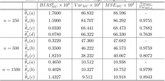
BIAS2 M C 103 V arM C 103 M SEM C 103 _{V ar}V arM C M C;a b_n(a) 1.7600 86.832 88.596 -n = 250 ebn(b) 1.5900 84.707 86.292 0.9755 ee_n(c) 0.0330 68.441 68.473 0.7882 es_n(d) 0.0780 66.322 66.330 0.7638 b_n(a) 0.3220 47.360 47.682 -n = 500 ebn(b) 0.3500 46.222 46.573 0.9759 ee_n(c) 1.8210 38.232 40.067 0.8072 bn(a) 0.4650 10.512 10.938 -n= 1500 ebn(b) 0.4028 10.327 10.752 0.9799 ee_n(c) 1.4327 9.512 10.918 0.8943

A brief summary of MC results: First, the MC variances of all the estimators (a), (b), (c)

and (d) decrease approximately linearly as the sample size increases. The QQ plots, which are not reported here for length considerations, indicate that all the four estimators are root-nasymptotically normal. Second, the e¢ cient estimators, (c) and (d), have lower MC variances than the ine¢ cient simple plug-in estimator (a). Third, the MC variance gap between the estimators (or the …nite sample e¢ ciency gain) is bigger for the “high-endogeneity”case.5 _{Lastly, the variance gap decreases}

as the sample size n increases. All of these …ndings are consistent with our theoretical results.

5_{The particular magnitude of the …nite sample e¢ ciency gain directly depends on the value of (the exogenous}

noise level). In MC studies that are not reported here, we discover that smaller values lead to smaller biases and smaller variances in the e¢ cient estimators; hence bigger MC variance gaps.

Table 2: Monte Carlo Results for “mid-endogeneity” case. BIAS2 M C 103 V arM C 103 M SEM C 103 _{V ar}V arM C M C;a b_n(a) 0.3420 79.246 79.590 -n = 250 ebn(b) 0.2751 77.164 77.433 0.9716 ee_n(c) 0.1810 70.005 70.186 0.8717 es_n(d) 0.3110 67.700 68.011 0.8530 b_n(a) 0.2010 37.503 37.704 -n = 500 ebn(b) 0.1860 36.951 37.137 0.9853 ee_n(c) 0.2200 33.794 33.974 0.9064 bn(a) 0.0200 9.2042 9.2244 -n= 1500 ebn(b) 0.0201 9.1928 9.2132 0.9987 ee_n(c) 0.1062 8.6932 8.7996 0.9444

5

Conclusion

In this paper we computed the semiparametric e¢ ciency bound for …nite dimensional parameters of sequential moment restriction models (1) containing unknown functions that may depend on endogenous variables. The results extend those of Chamberlain (1992b), Ai and Chen (2003) and Chen and Pouzo (2009) to the case of semi/nonparametric conditional moment restriction with nested information sets. The results also extend those of Chamberlain (1992a), and Brown and Newey (1998) to the case of sequential moment restrictions involving unknown functions. Our characterization of the e¢ ciency bound is useful in evaluating and comparing several competing estimators that are typically proposed for a particular semiparametric econometric model. Although we can only characterize the e¢ ciency bounds for conditional moment models involving several unknown functions when they depend on di¤erent arguments, these bounds can be computed analytically for many speci…c models containing only one unknown function. In terms of semiparametric e¢ ciency bound calculation, our approach carries over to allow for T to increase to in…nity. However, any e¢ cient estimation method would face the “curse-of-dimensionality” when T is very large.

We present an optimally weighted, orthogonalized SMD estimation procedure for ( o; ho)

identi-…ed by the sequential moment restriction model (1). When the semiparametric e¢ ciency bound for

o is non-singular, we note that this estimator is root-n asymptotically normal and e¢ cient for o.

There are many alternative procedures that can also achieve the semiparametric e¢ ciency bound for o in model (1). For instance, one could extend the constrained sieve MLE approach of Gallant

and Tauchen (1989), Gallant, Hansen and Tauchen (1990) and Ai (2007) to estimate o e¢ ciently.

Notice that ( o; ho) in model (1) is the unique solution to

E[ _t(Z; o; ho( )) p kt;n t (X (t)_{)] = 0 fort = 1; :::; T, (21)} where pkt;n t (X(t)) = (pt;1(X(t)); : : : ; pt;kt;n(X

(t)₎₎0 _{is a series of basis functions that can approximate}

any square integrable function of X(t) _{arbitrarily well as k}

t;n ! 1. One could also estimate o in

(21) by extending the GMM with increasing number of unconditional moments of Hahn (1997), or the continuum GMM of Carrasco and Florens (2000), or the empirical likelihood with increasing number of unconditional moments of Donald, Imbens and Newey (2003). We shall investigate these alternative e¢ cient procedures in another paper.

References

[1] Ai, C. (2007): “A Nonparametric Maximum Likelihood Estimation of Conditional Moment Restrictions Models”, International Economic Review, 48(4), 1093 - 1118.

[2] Ai, C. and X. Chen (2003): “E¢ cient Estimation of Conditional Moment Restrictions Models Containing Unknown Functions,”Econometrica,71, 1795-1843.

[3] Ai, C. and X. Chen (2007): “Estimation of Possibly Misspeci…ed Semiparametric Conditional Moment Restriction Models With Di¤erent Conditioning Variables,”Journal of Econometrics, 141, 5-43.

[4] Andrews, D. (1991) “Asymptotic Normality of Series Estimators for Nonparametric and Semi-parametric Regression Models”, Econometrica,59, 307-345.

[5] Antoine, B., H. Bonnal and E. Renault (2007) “On the E¢ cient Use of the Informational Content of Estimating Equations: Implied Probabilities and Euclidean Empirical Likelihood”, Journal of Econometrics, 138, 461-487.

[6] Begun, J., W. Hall, W. Huang, and J. Wellner (1983): “Information and Asymptotic E¢ ciency in Parametric-Nonparametric Models,” Annals of Statistics, 11, 432–452.

[7] Bickel, P. J., C. A. J. Klaassen, Y. Ritov, and J. A. Wellner (1993): E¢ cient and Adaptive Inference in Semiparametric Models. Johns Hopkins University Press, Baltimore.

[8] Blundell, R., X. Chen and D. Kristensen (2007): “Semi-nonparametric IV Estimation of Shape-Invariant Engel Curves,”Econometrica, 75, 1613-1670.

[9] Brown, B. and W. Newey (1998): “E¢ cient Semiparametric Estimation of Expectations,”

Econometrica, 66, 453-464.

[10] Carrasco, M. and J. P. Florens. 2000. Generalization of GMM to a Continuum of Moment Conditions. Econometric Theory 20:797-834.

[11] Carrasco, M., J. P. Florens and E. Renault 2007. Linear Inverse Problems in Structural metrics Estimation Based on Spectral Decomposition and Regularization. Handbook of Econo-metrics, Vol. 6B, eds. J.J. Heckman and E.E. Leamer. North-Holland, Amsterdam.

[12] Chamberlain, G. 1987. Asymptotic E¤ciency in Estimation with Conditional Moment Restric-tions. Journal of Econometrics 34:305-334.

[13] Chamberlain, G. (1992a) “Comment: sequential moment restrictions in panel data,”Journal of Business and Economic Statistics 10, 20-26.

[14] Chamberlain, G. (1992b) “E¢ ciency Bounds for Semiparametric Regression,”Econometrica, 60, 567-596.

[15] Chen, X., 2007. Large Sample Sieve Estimation of Semi-Nonparametric Models, Chp. 76 in Handbook of Econometrics, Vol. 6B, eds. J.J. Heckman and E.E. Leamer. North-Holland, Am-sterdam.

[16] Chen, X. and D. Pouzo (2009): “E¢ cient Estimation of Semiparametric Conditional Moment Models with Possibly Nonsmooth Residuals,”Journal of Econometrics 152, 46-60.

[17] Chen, X. and D. Pouzo, 2008a. Estimation of Nonparametric Conditional Moment Models with Possibly Nonsmooth Moments. Cowles Foundation Discussion Paper 1650.

[18] Chen, X. and D. Pouzo, 2008b. E¢ cient Estimation of Nonparametric Quantile IV Weighted Average Derivative. Mimeo, Yale University and New York University.

[19] Chernozhukov, V. and H. Hong. 2003. An MCMC Approach to Classical Estimation. Journal of Econometrics 115:293-346.

[20] Chernozhukov, V., G. Imbens, and W. Newey. 2007. Instrumental Variable Estimation of Non-separable Models. Journal of Econometrics 139, 4-14.

[21] Darolles, S., J.-P. Florens and E. Renault (2002): “Nonparametric Instrumental Regression,” mimeo, GREMAQ, University of Toulouse.

[22] Donald, S., G. Imbens and W. Newey (2003): “Empirical Likelihood Estimation and Consistent Tests with Conditional Moment Restrictions,”Journal of Econometrics, 117, 55–93.

[23] Gallant, A. R., L. P. Hansen, and G. Tauchen (1990): “Using Conditional Moments of As-set Payo¤s to infer the Volatility of Intertemporal Marginal Rates of Subsitution,” Journal of Econometrics, 45(2), 141–179.

[24] Gallant, A. R., and G. Tauchen (1989): “Seminonparametric Estimation of Conditionally Con-strained Heterogeneous Processes: Asset Pricing Applications,”Econometrica, 57(5), 1091–1120. [25] Hahn, J. (1997) “E¢ cient estimation of panel data models with sequential moment restrictions,”

Journal of Econometrics 79, 1-21.

[26] Hall, P. and J. Horowitz (2005): “Nonparametric Methods for Inference in the Presence of Instrumental Variables,” Ann of Statistics, 33, 2904-2929.

[27] Hansen, L.P. (1982): “Large Sample Properties of Generalized Method of Moments Estimators,”

Econometrica, 50, 1029-1054.

[28] Hansen, L.P. (1985): “A method for calculating bounds on the asymptotic covariance matrices of generalized method of moments estimators,”Journal of Econometrics, 30, 203-238.

[29] Hansen, L.P. (1993): “Semiparametric e¢ ciency bounds for linear time-series models,”in Mod-els, Methods, and Applications of Econometrics: Essays in Honor of A. R. Bergstrom, edited by PCB Phillips, Cambridge, MA: Blackwell.

[30] Hansen, L.P. (2007). Generalized Method of Moments, entry for the New Palgrave Dictionary of Economics, 2nd edition: edited by S. Durlauf and L. Blume. New York: Elsevier.

[31] Hansen, L.P., J. Heaton, and M. Ogaki (1988): “E¢ ciency Bounds Implied by Multiperiod Conditional Moment Restrictions,” Journal of the American Statistical Association, 83, 863– 871.

[32] Hayashi, F., and C. Sims, 1983: “Nearly e¢ cient estimation of time series models with prede-termined, but not exogenous, instruments. Econometrica, 51, 783–798.

[33] Kitamura, Y., G. Tripathi and H. Ahn (2004) “Empirical Likelihood-based Inference in Condi-tional Moment Restriction Models”,Econometrica, 72, 1667-1714.

[34] Newey, W. 1990. “Semiparametric E¢ ciency Bounds,”Journal of Applied Econometrics, 5, 99-135.

[35] Newey, W. 1993. E¢ cient Estimation of Models with Conditional Moment Restrictions. In Hand-book of Statistics, vol. 11, edited by G. S. Maddala, C. R. Rao, and H. D. Vinod. Amsterdam: North Holland.

[36] Newey, W., 1997. Convergence rates and asymptotic normality for series estimators. Journal of Econometrics, 79, 147-168.

[37] Newey, W., 2004. E¢ cient Semiparametric Estimation via Moment Restrictions,Econometrica,

72, 1877-1897.

[38] Newey, W. and J. Powell (2003) “Instrumental Variable Estimation of Nonparametric Models”,

Econometrica,71, 1565-1578.

[39] Newey, W. and R. Smith (2004) “Higher Order Properties of GMM and Generalized Empirical Likelihood Estimators”,Econometrica, 72, 219-256.

[40] Newey, W. and T. Stoker, 1993, E¢ ciency of Weighted Average Derivative Estimators and Index Models, Econometrica, 61, 1199-1223.

[41] Otsu, T. (2007) “Sieve Conditional Empirical Likelihood Estimation of Semiparametric Models”, forthcoming inEconometric Theory.

[42] Stein, C. (1956): “E¢ cient Nonparametric Testing and Estimation,”in Proceedings of the Third Berkeley Symposium in Mathematical Statistics and Probability, vol. 1, pp. 187–196, Berkeley University of California Press.

Mathematical Appendix

We follow the approach of Stein (1956), Begun, Huang and Wellner (1983), Bickel, et al. (1993), Newey (1990), Chamberlain (1992a, b), and van der Vaart (1991) on semiparametric e¢ ciency bound calculation. Recall the following notation for any _{2 A}:

"T(Z; ) T(Z; ); "s(Z; ) s(Z; ) T X t=s+1 s;t(X(t))"t(Z; )for s=T 1; :::;1; s;t(X(t)) E[ s(Z; o)"t(Z; o)0jX(t)]f ot(X(t))g 1fors < tand ot(X(t)) E["t(Z; o)"t(Z; o)0jX(t)].

Also, recall that

E_f"s(Z; o)"t(Z; o)v(X(s))q(X(t))g= 0 (22)

holds for any s ₆= t and for any measurable functions v and q. Finally we denote mt(X(t); )

E["t(Z; )jX(t)] for t= 1; :::; T.

Denote dz = dim(Z). Let po( ) be the true probability density of Z = (Y0; X0)0 with respect to

a sigma-…nite measure on _{Z R}dz _{that satis…es model (1), which is equivalent to the following}

model:

E["t(Z; o)jX(t)] = 0 for t= 1; :::; T and o 2 A; (23)

whereE denotes expectation taken with respect to the true density functionpo(z). LetEpdenote

ex-pectation taken with respect to arbitrary density functionp(z). For arbitrary _{2 A}, the conditional moment restrictions

Ep["t(Z; ; h)jX(t)] = 0 for t= 1; :::; T (24)

do not uniquely determine p(z). For any _{2 A}, let _F denote all probability density functions that satisfy (24):

F = p( ) :

Z

z2Z

p(z)d (z) = 1; p( ) 0; Ep["t(Z; ; h)jX(t)] = 0 fort = 1; :::; T :

For any p( ) _{2 F} , we can always write p(z) f(z_j ; g) with po(z) f(zj o; go), where p is of a

known functional form up to unknown parameters and g, with g being an unknown measurable function of z (see Ai (2007) for an example). g(z)can be viewed as the remainder of the probability density function p(z) f(z_j ; g) that is not determined by (24), and is unrestricted except for satisfying f(_j ; g) _{2 F} and f(_j o; go) 2 F o. Let G denote a class of real valued measurable

functions of Z satisfying (i) for each _{2 A},_ff(z_j ; g) :g _{2 Gg}=_F ; (ii) there is a go in the interior

of _G such that po(z) f(zj o; go).

The following condition shall be imposed throughout the paper.

Assumption A: Let _f( ( ); g( )) : ₂ [0;1]_g denote a family of parametric speci…cations in the parameter space _{A G} satisfying: (1) f(_j ( ); g( )) _{2 F} ( ); f(Zj (0); g(0)) = f(Zj o; go)

po(Z) holds with probability one; ! p

f(_j ( ); g( )) is mean-square di¤erentiable. (2) For all

j = 1; :::; T, with probability one, "j(Z; ( )) is continuous at ( ) in a small neighborhood of

= 0, dE["j(Z; ( ))jX(j)]

d j =0 and

dE["j(Z; o;h( ))jX(j)]

d j =0 exist and have …nite second moments, and

E[_j"j(Z; o)j2jX(j)]is bounded.

Proof. (Theorem 2.1) Let _f( ( ); g( )) : ₂ [0;1]_g be any parametric path in _{A G} satisfying

assumption A. Denote the log-likelihood function (of one observation) of a parametric submodel by

`(z; ( ); g( )) = logf(z_j ( ); g( )). Under assumption A, we can write the pathwise derivative of

`(z; ( ); g( )) at( o; go)as r`(z; o; go) = lim !0 `(z; ( ); g( )) `(z; o; go) = ` (z; o; go) d ( ) d j =0+`h(z; o; go) dh( ) d j =0+`g(z; o; go) dg( ) d j =0 = ` (z; o; go) +`h(z; o; go) [ h] +`g(z; o; go) g;

where the second and the third term on the right-hand side denote the pathwise derivative with respect to h and g respectively. To simplify notation we denote ` (z) ` (z; o; go), `h(z)[ h]

`h(z; o; go)[

dh( )

d j =0]and`g(z) g(z) `g(z; o; go)

dg( )

d j =0. Notice that anyp(z) = f(zj ( ); g( )) 2

F ( ) satis…es restrictions (24). By di¤erentiating both sides of (24), we obtain: dE["j(Z; o)jX(j)] d +E["j(Z; o)` (Z)jX (j)<sub>] = 0 for j = 1; :::; T; (25)</sub> dE["j(Z; o; h( ))jX(j)] d j =0+E["j(Z; o)`h(Z) [ h]jX (j)_{] = 0 for j = 1; :::; T; (26)} E["j(Z; o)`g(Z) g(Z)jX(j)] = 0 for j = 1; :::; T: (27) Denote Th = ah( ) =`h( )[ h] :E[ah(Z)] = 0; E[fah(Z)g2]<1; h2 H fhog; (26) holds :

Tg = ag( ) = `g( ) g( ) :E[ag(Z)] = 0; E[fag(Z)g2]<1; (27) holds :

Let _Th and Tg respectively denote the closed linear completions of Th and Tg under the mean

squared norm _kv( )_k2₂ = E_fv(Z)2_g. Then _Th and Tg are the tangent spaces for the nonparametric

parameters h and g respectively. Denote _T = _Th +Tg. Let Proj(jT) denote the population least

square projection of onto the space _T. The semiparametric e¢ cient score of o is given by S

` (Z) proj(` (Z)_jT) (see, e.g., Bickel et al. 1993). Denote Jo E[S S 0] as the semiparametric

Fisher information bound. IfJo is non-singular, then the semiparametric e¢ cient variance bound for

o is (Jo) 1 (E[S S 0])

1

.

To compute the least squares projections, note that, for each component k (of ), k = 1; :::; d , the projection proj(` k(Z)jT)solves the following minimization problem:

E ` k(Z) proj(` k(Z)jT) 2 E ` k(Z) a<sub>h</sub>(Z) a<sub>g</sub>(Z) 2 = min ah2Th;ag2Tg E [` k(Z) a_h(Z) a_g(Z)]2 = min ah2Th min ag2Tg E [` k(Z) a<sub>h</sub>(Z) a<sub>g</sub>(Z)]2 = min ah2Th n E ` k(Z) a_h(Z) proj(` k(Z) a_h(Z)jT_g) 2 o ;

where a_{h 2T}h; ag proj(` k(Z) ah(Z)jTg)2Tg denote a pair of solutions.

For anyah =`h( )[ h]2Th (with h2 H fhog), to compute a solution proj(` k(Z) a_h(Z)jT_g)

to the problem min_a

g2Tg E[` k(Z) ah(Z) ag(Z)]

2

, we write the Lagrangian expression as

E ( [` k(Z) a_h(Z) a_g(Z)]2+ 2 T X j=1 j(X(j))0"j(Z; o)ag(Z) ) ; (28)

where j(X(j)) is the Lagrangian multiplier for the constraint (27). Applying calculus of variation,

any solution ag to the unconstrained minimization problem (28) should satisfy the following …rst

order condition: ` k(Z) a_h(Z) a_g(Z) = T X j=1 j(X(j))0"j(Z; o); (29) E["j(Z; o) ag(Z)jX(j)] = 0 for j = 1;2; :::; T:

de…nition of "j(Z; o); j = 1;2; :::; T and relation (22), it is straightforward to show that t(X(t))0 = dmt(X(t); o) d k dmt(X(t); o) dh [ h] 0 ot(X(t)) 1; t= 1;2; :::; T solves (29). Hence ag(Z) =` k(Z) a_h(Z) T X t=1 t(X(t))0"t(Z; o)

solves the unconstrained minimization problem (28). Moreover, becauseE_f[` k(Z)]2g<1,Ef[a_h(Z)]2g<

1, En t(X(t))0"t(Z; o)

2

e o

<₁, we have E_f[ag(Z)]2g<1 and ag 2Tg. Thus

proj(` k(Z) a<sub>h</sub>(Z)jT<sub>g</sub>) =a<sub>g</sub>(Z) =` k(Z) a_h(Z)

T X

t=1

t(X(t))0"t(Z; o):

That is, for any ah =`h( )[ h]2Th (with h2 H fhog), we have:

` k(Z) a<sub>h</sub>(Z) proj(` k(Z) a_h(Z)jT_g) (30) = T X t=1 dmt(X(t); o) d k dmt(X(t); o) dh [ h] 0 ot(X(t)) 1"t(Z; o):

Recall that the space _W is the closed linear completion of _{H f}hog under the pseudo-normjj jj

k h_k2 E " _T X t=1 dmt(X(t); o) dh [ h] 0 ot(X(t)) 1 dmt(X(t); o) dh [ h] # <₁:

For any direction h _{2 H f}hogwithah =`h( )[ h]2Th, given assumptions 2, 3 and A and relation

(30), we have_k h_k2 <₁hence this direction hbelongs to_W. Conversely, for any eh_{2 H f}hog

with eh 2

<₁ (so that eh_{2 W}), de…ne

eah(z) = T X t=1 dmt(X(t); o) dh [ eh] 0 ot(X(t)) 1"t(z; o):

It is obvious thatE[_eah(Z)] = 0. By de…nition ofWand eh2 Wwe haveE[feah(Z)g2] = eh

2 <₁.

Also relation (22) implies that

dmj(X(j); o)

dh [ eh] +E[eah(Z)"j(Z; o)

0_jX(j)_{] = 0 for j = 1; :::; T;}

thus _eah( )2Th.

By de…nitions of_Th,Th andah(), there exists a sequencefwh;j 2 H fhog; j = 1;2; :::gsuch that

ah;j( ) =`h( ) [wh;j]2Th converges toah( )2Thunder the mean-squared norm. Since the projection

is a bounded linear functional, ag;j(Z) proj(` k(Z) a_h;j(Z)jT_g)converges toa_g(Z)2T_g under the

mean-squared norm. By de…nition of _W, such a sequence _fwh;j 2 H fhog; j = 1;2; :::g belongs to

W. By relation (30), we have: 1 > E ` k(Z) a<sub>h;j</sub>(Z) proj(` k(Z) a_h;j(Z)jT_g) 2 = E " _T X t=1 f ot(X(t))g 1 2 dmt(X (t)_; o) d k dmt(X(t); o) dh [wh;j] 2 e # E " _T X t=1 f ot(X(t))g 1 2 dmt(X (t)_; o) d k dmt(X(t); o) dh [r k o] 2 e # ; (31)

where the last inequality is due to the fact that rk

o is a solution to inf w2W E " _T X t=1 f ot(X(t))g 1 2 dmt(X (t)_; o) d k dmt(X(t); o) dh [w] 2 e # :

Taking limit as j _{! 1}in both sides of inequality (31), we obtain:

E ` k(Z) a_h(Z) a_g(Z) 2 E " _T X t=1 f ot(X(t))g 1 2 dmt(X (t)_; o) d k dmt(X(t); o) dh [r k o] 2 e # : (32) On the other hand, by de…nitions of _W and rk

o, there exists a subsequence fweh;j 2 H fhog; j =

1;2; :::_g in _W such that 1> E " _T X t=1 f ot(X(t))g 1 2 dmt(X (t)_; o) d k dmt(X(t); o) dh [weh;j] 2 e #

converges to E " _T X t=1 f ot(X(t))g 1 2 dmt(X (t)_; o) d k dmt(X(t); o) dh [r k o] 2 e # asj _{! 1}: Let e ah;j(z) = T X t=1 dmt(X(t); o) dh [weh;j] 0 ot(X(t)) 1"t(z; o):

Then _eah;j( )2Th and hence eag;j(z) proj(` k(Z) ea_h;j(Z)jT_g)2T_g, we have

E " _T X t=1 f ot(X(t))g 1 2 dmt(X (t)_; o) d k dmt(X(t); o) dh [weh;j] 2 e # = E ` k(Z) ea<sub>h;j</sub>(Z) proj(` k(Z) ea_h;j(Z)jT_g) 2 E ` k(Z) a_h(Z) a_g(Z) 2 : (33) Taking limit (as j _{! 1}), and combining with the previous inequality (32), we obtain

E ` k(Z) proj(` k(Z)jT) 2 E ` k(Z) a_h(Z) a_g(Z) 2 = E " _T X t=1 f ot(X(t))g 1 2 dmt(X (t)_; o) d k dmt(X(t); o) dh [r k o] 2 e # : Denotero = (ro1; :::; rod ) and dmt(X(t); o) dh [ro] = dmt(X(t); o) dh [r 1 o]; dmt(X(t); o) dh [r 2 o]; :::; dmt(X(t); o) dh [r d o ] :

Then, an e¢ cient score S for o is

S ` (Z) proj(` (Z)_jT) = T X t=1 dmt(X(t); o) d 0 dmt(X(t); o) dh [ro] 0 ot(X(t)) 1"t(Z; o):

The semiparametric Fisher information bound for o isJo E[S S 0], and ifJo is non-singular, then

the semiparametric e¢ cient variance bound for o is (Jo) 1 (E[S S 0]) 1.

When we partition into( 0₁; 0₂)0 _withd

i = dim( i)and d =d 1+d 2 for i= 1;2, we let ro 1 (r_o1; :::; rd1 o )2Q d₁ j=1W,ro 2 (r d₁+1 o ; :::; rod )2 Qd₂ j=1W, dm1(X; o) dh [ro 1] ( dm1(X; o) dh [r 1 o]; :::; dm1(X; o) dh [r d₁ o ])