On the Bayesian calibration of computer model mixtures through experimental data, and the design of predictive models.

Durham Research Online

Deposited in DRO:

22 August 2017

Version of attached le:

Peer-review status of attached le:

Citation for published item:

Karagiannis, G. and Lin, G. (2017) 'On the Bayesian calibration of computer model mixtures through

experimental data, and the design of predictive models.', Journal of computational physics., 342 . pp. 139-160.

Further information on publisher's website:

https://doi.org/10.1016/j.jcp.2017.04.003 Publisher's copyright statement:

c

2017 This manuscript version is made available under the CC-BY-NC-ND 4.0 license http://creativecommons.org/licenses/by-nc-nd/4.0/

Additional information:

Use policy

The full-text may be used and/or reproduced, and given to third parties in any format or medium, without prior permission or charge, for personal research or study, educational, or not-for-prot purposes provided that:

• a full bibliographic reference is made to the original source

• alinkis made to the metadata record in DRO

• the full-text is not changed in any way

The full-text must not be sold in any format or medium without the formal permission of the copyright holders. Please consult thefull DRO policyfor further details.

On the Bayesian calibration of computer model mixtures through

experimental data, and the design of predictive models

Georgios Karagiannisa_{, Guang Lin}b

a_{Department of Mathematical Sciences, Durham University, Stockton Road, Durham, DH1 3LE, UK} b_{Department of Mathematics, School of Mechanical Engineering, Purdue University, West Lafayette, IN 47907, USA}

Abstract

For many real systems, several computer models may exist with different physics and predictive abilities. To achieve more accurate simulations/predictions, it is desirable for these models to be properly combined and calibrated. We propose the Bayesian calibration of computer model mixture method which relies on the idea of representing the real system output as a mixture of the available computer model outputs with unknown input dependent weight functions. The method builds a fully Bayesian predictive model as an emulator for the real system output by combining, weighting, and calibrating the available models in the Bayesian framework. Moreover, it fits a mixture of calibrated computer models that can be used by the domain scientist as a mean to combine the available computer models, in a flexible and principled manner, and perform reliable simulations. It can address realistic cases where one model may be more accurate than the others at different input values because the mixture weights, indicating the contribution of each model, are functions of the input. Inference on the calibration parameters can consider multiple computer models associated with different physics. The method does not require knowledge of the fidelity order of the models. We provide a technique able to mitigate the computational overhead due to the consideration of multiple computer models that is suitable to the mixture model framework. We implement the proposed method in a real world application involving the Weather Research and Forecasting large-scale climate model.

Keywords: Uncertainty quantification, computer experiments, Gaussian process, polynomial bases, multinomial logistic model, MCMC

1. Introduction

Computer experiments often use computer models (simulators) to simulate the behavior of a complex real system under consideration. These models are usually designed according to theories believed to govern the real system. They usually include calibration parameters, that is unknown parameters that regulate the behavior of the computer model; hence we wish to tune (calibrate) them in order for the computer model to

Email addresses: [email protected], [email protected](Georgios Karagiannis),

represent the real system accurately. Often, calibration of a computer model is performed in the presence of experimental data in order to find optimal values for the unknown calibration parameters. In cases that the computer models are expensive to run, there is interest in building inexpensive predictive statistical models. Kennedy and O’Hagan [1] proposed an effective Bayesian computer model calibration to address such cases. Briefly, the experimental observations are represented as a sum of three functional terms: the computer model output, a systematic discrepancy, and an observational error. These functional terms are modeled as Gaussian processes [1, 2, 3, 4], because computer models are often computationally expensive, and available training data are limited. Literature includes several variations of computer model calibration which can handle different issues; e.g. discontinuity/non-stationarity in the outputs [5], discrete inputs [6], calibration in the frequentest context [7], high-dimensional outputs [8], dynamic discrepancy [9], large number of inputs and outputs [10], etc. However, these works are restricted in cases where a single computer model is available. Nowadays, there is a plethora of computer models that aim at simulating the same real system. These models may differ either in precision (multi-fidelity case) of the solvers involved, or in the theories based on which they are designed (multi-physics case). Recently, Goh et al. [11] proposed a procedure to perform Bayesian calibration of computer models available at different levels of fidelity. It combines the models in a nested structure according to a given fidelity order. However, this approach is restricted to address only multi-fidelity cases where the fidelity order of the computer models is known.

Often, there are available several computer models, based on different theories, that represent the same real system. Each single computer model may have its own unique properties and predictive capabilities in representing the real system. Therefore, there is not a commonly acceptable way to order such models. Possible reasons for example can be: (i) incomplete knowledge of the complex real system, (ii) different computational capabilities of research groups, (iii) different scientific theories or perspectives describing the same real system, etc. In such cases, using only a single computer model may lead to misleading inferences and predictions and ignore the physics considered by other computer models only. Furthermore, traditional multi-fidelity calibration methods, such as [11], are not suitable to address such cases because the fidelity order of the models is not available a priori, or because nesting one model to another could possibly impose unrealistic relations among the models. Moreover, in the presence of moderately large number of models, the direct implementation of standard multi-fidelity calibration method becomes very expensive. Here, the question of interest is how to properly combine and calibrate such computer models in order to represent the real system output accurately.

In this study, the motivation for addressing the aforesaid problem raises from the Weather Research and Forecasting (WRF) regional climate model [12]. WRF allows for different configurations (sub-models), e.g. different parametrization suits, physics schemes, or resolutions, which in principle can constitute different models. Briefly, here the available computer models consist of different combinations of radiation schemes,

(the Rapid Radiative Transfer Model for General Circulation Models [13], and the Community Atmosphere Model 3.0 [14]) that describe different physics, and different resolutions (25km and50km grid spacing) that describe different fidelity levels. It is uncertain which radiation scheme leads to better simulations. Moreover, higher grid spacing does not necessarily lead to more accurate simulations because WRF is sensitive to other physical parametrizations which is uncertain how they are affected by the grid spacing. Combination of physics variability is expected to result better predictions in climate models [15]; hence interest lies in combining suitably these computer models in order to integrate the associated physics and fidelity variations. WRF is employed with the Kain Fritsch (KF) convective parametrization scheme (CPS) [16]. For climate models, it is important to better understand and constrain the convective parametrization, and hence interest lies in quantifying and reducing the uncertainties regarding of those parameters. The computational cost of running WRF is prohibitively high, and an exhausted direct simulation study is not possible in practice; hence there is interest in a predictive model.

In this article, we propose the Bayesian calibration of computer model mixture method, as an extension to the traditional Bayesian (single) model calibration [1, 2]. Central to the proposed methodology is the idea of (i) representing the output function of the complex real system as a mixture of output functions of the available computer models with unknown input dependent weight functions, and (ii) specifying a fully Bayesian model to quantify the associated uncertainties. The proposed method allows one to build a predictive model (emulator) for the output of a real system by properly calibrating, weighting, and combining the available computer models in the Bayesian framework. Additionally, it allows the design of a calibrated mixture of computer models (simulators) by evaluating the associated weight functions and the calibration parameters. The resulting computer model mixture, as well as the predictive model, aim at representing the real system output more accurately than the single ones by aggregating the unique features of different models. We introduce the concept of shared calibration parameters that allows inference on calibration parameters to be based on multiple computer models (and hence different physics), however, the method allows different models to have different calibration parameters. The Bayesian computations are performed via Markov chain Monte Carlo methods. A computational highlight of the procedure is that it builds the unknown mixture weight functions via a stochastic bases selection from a pool of basis functions in a data-driven manner.

The method is suitable to address realistic problems that one model may be more accurate than the other at different (unspecified) input sub-regions. In particular, through the weight functions, it allows the determination of the input sub-region at which a individual computer model is more preferable to be used than the rest individual ones. The method is particularly suitable to address applications where the outputs of the available computer models tend to differ from the output of the real system at different directions. This is because the weight functions can adjust the outputs of contributing models in the mixture, in a

manner that the overall discrepancy of the mixture will be less that the individual ones. Therefore, in such cases, the resulting calibrated computer model mixture is able to produce more accurate simulations than the single ones. This covers a large range of important real world applications [15], such as the WRF one analyzed here.

The article is organized as follows. In Section 2, we present the proposed method. In Section 3.1, we validate the proposed method with that of Goh et al. [11] in a validation example. In Section 3.2, we assess the good performance of the method and compare it with that of Kennedy and O’Hagan [1] in a more challenging benchmark example. In Section 3.3, we implement the method on a real world large-scale climate modeling application that involves the WRF with the KF CPS. In Section 4, we conclude and propose possible extensions. In AppendixB, we provide a technique that mitigates the computational overhead of the procedure which is caused by the consideration of multiple computer models.

2. The method

The proposed method extends the standard Bayesian calibration of a single computer model [1, 2] to the multiple computer model framework.

2.1. Basic formulation

Set-up. We assume there is available a set of K different computer models tSpkq; k P Ku where K “ t1, ..., Ku. Each computer modelSpkq _{aims at simulating the same real systemZ.}

We consider training data which consist of a collection of experimental data tpyi, xiq; i“1, ..., nu

gen-erated from the real system Z after n realizations, andK designs of simulated data tpη_ipkq, xp_ikq, tp_ikqq; i“

n`ř<sub>jăk</sub>mpjq<sub>`1, ..., n`</sub>ř

jďkmp

jq_{ugenerated from the computer modelS}pkq_aftermpkq_{runs fork“1, ..., K.}

LetzK_{“ p}y|, ηp1q,|, ..., ηpKq,|_qdenotes the complete training data outputs, andnK _“n_`řK

k“1mp

kq

de-notes the size of zK. Here, y

i PR, xi PX, x

pkq

i P X, and t

pkq

i P Θpkq, for any i,k, where X is the input

domain, andΘpkq _{is the calibration parameter domain of computer model}Spkq_.

Regarding the real systemZ, the experimental observationsyi:“ypxiqare generated for a givenxivia

yi“ζpxiq `y,i,

where the y,i denotes the observation error, and ζpxiq denotes the expected output of the real system at

inputxi fori“1, ..., n.

Regarding the computer modelSpkq_{, the simulated dataη}pkq

i :“ηp

kq_pxpkq

i , t

pkq

i qare generated for a given

xp_ikq, and calibration parameters tp_ikq via

η_ipkq“Spkq

wherep_η,ikqdenotes the random error, andSpkq_pxpkq

i , t

pkq

i qdenotes the expected output of the computer model

Spkq_atpxpkq i , t pkq i q, fori“n` ř jăkmp jq<sub>`1, ..., n`</sub>ř jďkmp

jq_{. The inclusion of term}pkq

η as random error

is necessary whenSpkq _{is stochastic, as well as beneficial, in terms of the stability of the statistical model,}

whenSpkq _{is deterministic as discussed by Gramacy and Lee [17].}

Computer model mixture. Although each computer model aims at simulating the same real system, it may be designed based on different theoretical background and present different properties. In order to aggregate different properties associated with different computer models, we model the output function of the real system Z as a mixture of the output functions of the available computer models plus a discrepancy. He define the computer model mixture representation of the real system, as

SK_p¨, θK_{q “} K

ÿ

k“1

$kp¨qSpkqp¨, θpkqq; ζp¨q “SK_p¨, θK_{q `}δ_p¨q. (2.1)

Note that in our framework, the components of mixture (2.1) are computer models (simulators), unlike other works [18, 19, 20] in the literature where the components are different statistical models referring to the same computer model.

The main role of the weight functionst$kp¨quis to adjust the contribution of the corresponding computer

models tSpkq_{uin the mixture tS}K_u as functions of the input in a principled manner; for this reason we

consider them as a probability vector that depends on the inputs. Precisely,$p¨q:“ p$kp¨q;kP1, ..., Kqis the

unknown vector of weight functions such thatt$kp¨q:X Ñ p0,1q;k“1, ..., K´1u, and$Kp¨q:X Ñ p0,1q

with $Kp¨q “ 1´ř_kK_“´₁1$kp¨q. This allows differently weighted combinations of the computer models to

represent the real system at different inputs. Hence, (2.1) is suitable to model realistic problems where the unknown fidelity order of the computer models may change over the input space X. Moreover, δp¨q is a discrepancy function, and it refers to a potential systematic disagreement between the real system outputζp¨qand the computer model mixture outputSKp¨, θKq, e.g. due to ‘missed’ or ‘missrepresented’

physical properties. We highlight that different computer modelstSpkqumay have calibration parameters different in value, or dimensionality. As a result, there is need to evaluate the set of calibration parameters tθpkq_PΘpkq_{;kPKu, (orθ}K_{“ p}θp1q, ..., θpKq_q).

The computer model mixture calibration problem can be summarized as

CK: $ ’ ’ ’ ’ ’ ’ ’ ’ & ’ ’ ’ ’ ’ ’ ’ ’ % ypxiq “ řK k“1$kpxiqSpkqpxi, θpkqq `δpxiq `y,i, i“1, ..., n η_ip1q“Sp1q_pxp1q i , t p1q i q ` p1q η,i, i“n`1, ..., n`mp 1q .. . ... η<sub>i</sub>pKq“SpKq<sub>px</sub>pKq i , t pKq i q ` pKq η,i , i“n` ř kăKmp kq<sub>`1, ..., n</sub>K . (2.2)

Weight functions parametrization . The unknown weight functionst$kp¨qu are modeled a polynomial

ex-pansion in the multivariate logistic space, as

logp$kp¨q $Kp¨q q “gkp¨q; (2.3) gkp¨q “ ÿ aPΛ_{p$ ,dx} hpkq $,ap¨qωk,a, (2.4) for k “ 1, ..., K ´1, where $Kp¨q “ 1´ř K´1

k“1 $kp¨q, and gkp¨q is a polynomial expansion of degree p$.

Specifically,thp$,akqp¨quare multi-dimensional basis functions properly specified, for example from Askey family

[21],tωk,auare unknown coefficients, andΛp$,dxis a set of multi-indices indicating the available bases up to a

degreep$. The rational in (2.3) is that the additive logistic transformation is suitable to provide a monotonic

mapping between_RK´1_{and the simplex ofK-dimensional probability vector. Moreover, regarding (2.4), the} polynomial expansions are able to accurately represent unknown functions under certain regularity conditions [22].

Often, only a subset Ik PΛp,dx of bases significantly contributes to the expansion (2.4), while the rest

bases can be omitted without serious loss of accuracy [23]. Here, we consider that given a set of available bases Λp,dx, there is an unknown subset of significant bases with indices Ik Ă Λp,dx, for k “ 1, ..., K.

Therefore, given (2.4) using only the subset of bases with indicesIkĂΛp,dx, the unknown weight functions

result from the inversion of (2.3) as

$kp¨q “ expphp_$,kq_I kp¨q |_ω k,Ikq 1`řK_j“´₁1expphp_$,kq_I kp¨q |_ωj,I kq , (2.5) where hp_$,kq_I kp¨q :“ ph pkq

$,ap¨q;a P Ikq and ωk,Ik :“ pωk,a;a P Ikq for k “ 1, ..., K ´1, and $Kp¨q “

1´řK_k“´₁1$kp¨q. The consideration of smaller sets of bases thp

kq

$,ap¨q;a P Iku may have computational

benefits as it reduces the number of the unknown coefficientstωk,a;aPIkuto be estimated [23, 24, 25, 26].

Parametrization (2.5) leads to convenient computations, as well as reliable inferences and predictions. In the current framework, the use of Gaussian process priors [20] or an allocation model [27] for the repre-sentation of the weight functions would lead to expensive computations due to the introduction of many extra latent/nuisance variables. The special case where the weights are assumed to be constant values thp_$,kq_I

kp¨q “1uimplies that the fidelity of the computer models is constant across the input space, and hence

it can be too restrictive in real world problems.

Surrogate modeling. We consider the realistic scenario where the available computer models tSpkqu are computationally expensive, and hence they cannot be used directly in Bayesian computations that require a vast number of direct computer runs. The ‘uncertain’ functionstSpkq_{p¨,¨quandδp¨qare modeled as Gaussian}

processes (GP) [1, 4], that allow the design of an emulator for the output function in a mathematically convenient manner. ForkPK, we assign independent Gaussian processes priors on the functions Spkq_p¨,¨q

andδp¨qasSpkq_{p¨,¨q „GPpµ}pkq S p¨,¨q, c pkq S pp¨,¨q,p¨,¨qqq, andδp¨q „GPpµδp¨q, cδp¨,¨qq, whereµp kq S :XˆΘp kq_Ñ R,

µδ :X ÑRare the mean functions of the GPs, andcSpkq:XˆΘp

kq_ˆXˆΘpkq_Ñ

R`,cδ :XˆX ÑR` are

the covariance functions of the GPs. For presentation purpose, we consider a traditional parametrization forµp_Skqp¨,¨q, µδp¨q, cp

kq

S pp¨,¨q,p¨,¨qq, and cδp¨,¨q, however more intricate ones can be used in our framework.

The mean functions are specified as linear expansions µδp¨q “hδp¨q|βδ and µp

kq S p¨,¨q “h pkq S p¨,¨qβ pkq S where hδ:X ÑRdβ,δ andhSpkq:XˆΘpkqÑR dp_β,Skq

are vectors of basis functions, such as polynomial bases [21], or wavelets [28], andβδ,βp

kq

S are vectors of unknown coefficients withβ

pkq

S PR

dp_β,Skq

,βδ PRdβ,δ_{. The covariance}

functions can be specified according to the separable covariance function family [29, 30] as

cp_Skqppx, tq,px1_{, t}1 qq “τ_Spkq q ź l“1 pφp_S,x,lkq qp2|xl´x1l|q2 ppkq ź l“1 pφp_S,t,lkq qp2|tl´t1l|q2_{q; (2.6)} cδpx, x1q “τδ q ź l“1 pφδ,x,lqp2|xl´x 1 l|q 2 , (2.7)

where τ_Spkq ą 0, τδ ą0 control the marginal variances; tφp

kq

S,x,l P p0,1qu, tφ

pkq

S,t,l P p0,1q;u, tφδ,x,l P p0,1qu

control the dependence strength in each of the component directions ofxandt. More intricate covariance functions, such as the stationary ones from the Matérn family [31, 4], the non-stationary ones of Paciorek and Schervish [32], or the compact support (combined via tapering) ones [33, Chapter 9] can also be used in this set-up. Here,y andp

kq

η are modeled as random noises with unknown variances σy2ą0and σ

pkq,2

η ą0

respectively. We caution that some applications may requireyp¨qandtp

kq

η p¨,¨quto be treated as functions;

such a case is out of the scope of this article.

2.2. The Bayesian model

To facilitate the presentation we make the notation more compact, and define unknown random param-eters: θK :_{“ p}θp1q, ..., θpKq_q on spaceΘK, βK :_{“ p}βp1q S , ...β pKq S , β pkq δ q on spaceB K _: “R řK k“1d pkq β,S`dβ,δ_, ϕK :_{“ pp}φpkq S,x, φ pkq S,t, τ pkq S , σ pkq,2 η ;k“1, ..., Kq, φδ,x, τδ, σ2yqon spaceΦK, andI “ pI1, ...,IKq.

Statistical model. The (marginal) likelihood function of zK, marginalized with respect to the GP priors

of tSpkq_{p¨qu and δp¨q, is a multivariate Normal distribution with n}K-dimensional mean vector µK

z :“

µK

z pI, $, βK, θKqand covariance matrixΣzK :“ΣzKpI, $, ϕK, θKqof sizenKˆnK such that

µK z “ HK z “ hkkkkkkkkkkkkkkkkkkkkkikkkkkkkkkkkkkkkkkkkkkj » — — — — — — — — — – H_Sp1q H_Sp2q ¨ ¨ ¨ H_SpKq Hδ 9 H_Sp1q 0 ¨ ¨ ¨ 0 0 0 _H9p2q S . .. .. . ... .. . . .. . .. 0 0 0 ¨ ¨ ¨ 0 _H9pKq S 0 fi ffi ffi ffi ffi ffi ffi ffi ffi ffi fl βK_“ hkkkikkkj » — — — — — — — — — – βp_S1q βp_S1q .. . β_SpKq βδ fi ffi ffi ffi ffi ffi ffi ffi ffi ffi fl ; ΣK z “ » — — — — — — — — — – Σz Σp 1q,| z Σp 2q,| z ¨ ¨ ¨ Σp Kq,| z Σpz1q Σp 1,1q z 0 ¨ ¨ ¨ 0 Σzp2q 0 Σzp2,2q . .. ... .. . ... . .. . .. 0 ΣpzKq 0 ¨ ¨ ¨ 0 Σp K,Kq z fi ffi ffi ffi ffi ffi ffi ffi ffi ffi fl ,

respectively. Here, trH_Spkqsi,: “ $kpxiqhp kq,| S pxi, θpkqq;i “ 1, ..., n, k “ 1, ..., Ku, trHδsi,: “ h|δpxiq;i “ 1, ..., nu,trH9_Spkqsi,:“h pkq,| S pxi, t pkq i q;i“n` ř j1<sub>ăk</sub>mpj 1<sub>q</sub> `1, ..., n`ř<sub>j</sub>1<sub>ďk</sub>mpj 1<sub>q</sub> , k“1, ..., Ku, and rΣzsi,j“ K ÿ k“1 $kpxiq$kpxjqcp kq S ppxi, θpkqq,pxj, θpkqqq `cδpxi, xjq `σ2y10pi´jq, i“1, ..., n;j“1, ..., n; rΣpzkqsi,j“$kpxjqcp kq S ppxi, tp kq i q,pxj, θpkqqq, i“n` ÿ j1_ăk mpj1_q `1, ..., n` ÿ j1_ďk mpj1_q ;j “1, ..., n; rΣpzk,kqsi,j“cp kq S ppxi, tp kq i q,pxj, tp kq j qq `σ pkq,2 η 10pi´jq, i“n` ÿ j1_ăk mpj1_q `1, ..., n` ÿ j1_ďk mpj1_q ;j “n` ÿ j1<sub>ă</sub>k mpj1<sub>q</sub> `1, ..., n` ÿ j1_ďk mpj1_q , according to (2.6) and (2.7).

The proposed framework allows the introduction of shared calibration parameters, namely calibration parameters which are common to different computer models, have the same interpretation, and have the same values across different models. Different computer models, e.g. Spkq _and Spk1q_{, may share a set of}

common calibration parameters, e.g. θp_jkq andθ_jpk11q, that describe the same quantity. In many cases, it is desirable for some calibration parameters to be calibrated jointly across different models. Technically, this can be achieved by setting appropriate constrains on the spaceΘK, e.g. θpkq

j “θ

pk1_q

j1 . This allows inference on those parameters to be based on multiple computer models and hence possibly different physics. In the context of computer model mixture (2.2), the weight functions control the ‘contribution’ of each computer model in the calibration procedure through (2.1). Therefore, the training of shared calibration parameters is primary influenced by computer models with larger weights and hence those which represent the system output more accurately.

Prior model. We specify a prior model for the unknown parametersπpI, ω, βK, ϕK, θK_q.

Regarding the weight functions, we assign priors on Ik „PrpIkqin order to account uncertainty about

the unknown set of the significant bases functions, and Normal priors onωk „Npbω, ξω´1qin order to account

uncertainty about the unknown coefficients, for k“1, ..., K´1. A priori information, for example related to the fidelity of the computer models, can be included in the prior model by adjusting the prior hyper-parameters. Otherwise, weakly informative priors of the weight functions parameters can be used; e.g.

A priori independent priors can be assigned ontβK, ϕK_usuch that φp_S,x,lkq „Bepaφ,S,x, bφ,S,xq, l“1, ..., q; βp kq S „Npb pkq S , ξ ´1 β Σ pkq β,Sq; φp_S,t,lkq „Bepaφ,S,x, bφ,S,xq, l“1, ..., ppkq; βδ „Np0, ξ´β1Σβ,δq; φδ,x,l „Bepaφ,δ,x, bφ,δ,xq, l“1, ..., q; τ_Spkq „IGpaτ,S, bτ,Sq; σ2y „IGpaσ,y, bσ,yq; τδ „IGpaτ,δ, bτ,δq; σ pkq,2 η „IGpaσ,η, bσ,ηq, (2.8)

for k “ 1, ..., K, where Be and IG denote the Beta and inverse Gamma distributions. The fixed hyper-parameters in (2.8) are defined by the researcher. If no a priori information for tβ_Spkquandβδ is available,

one can letξβÑ0, so that ultimatelytβp

kq

S uandβδ are a priori completely unknown [3]. This limiting prior

‘distribution’ is improper, non-informative, and independent of the values of tbp_Skqu, tΣ_β,Spkqu, bδ, and Σβ,δ.

The priors assigned onφp_S,x,lkq,´1,φ_δ,x,lpkq,´1, andφp_S,t,lkq,´1are standard choices and suggested in [30]. The proposed methodology can be used even if different priors for the parameters of the covariance are specified.

Prior distribution on the calibration parameters πpθK_qis specified according to the available a priori

information. Available prior information about the dependency of calibration parameters, e.g. θpkq _and

θpk1_q

, between different computer models, e.g. Spkq _andSpk1_q

, can be included in the priors. Usually, the researcher is confident that the ideal values of the calibration parameters lie in a specific range, and hence the associated priors have positive mass over a bounded region ofΘK. In such cases, if a priori information

is available about a calibration parameter, one can assign truncated multivariate Normal prior distributions, otherwise one can assign uniform prior distributions.

Posterior model. The joint posterior distribution πpI, ω, βKϕK, θK|zKqaccording to the Bayes

theo-rem admits density

πpI, ω, θK, βK, ϕK_|zK_q9f_pzK_|ω, βK, ϕK, θK_qPr_pI_qπ_pω_|I_qπ_pβK_qπ_pϕK_qπ_pθK_q. (2.9)

It can be factorized as

πpI, ω, βK, ϕK, θK_|zK_{q “}π_pβK_|zK,I, ω, ϕK, θK_qπ_pI, ω, ϕK, θK_|zK_q (2.10)

where, on the right hand side of (2.10), the first distribution is a multivariate normal distribution

βK_|zK,I, ω, ϕK, θK_„N_pβˆK,WˆK_qwith mean and covariance matrix

ˆ βK _“WˆK_pHK,| z Σ K,´1 z z K `ξβΣ´β1bβq; (2.11) ˆ WK <sub>“ p</sub>HK,| z Σ K,´1 z H K z `ξβΣ´_β1q´1, (2.12)

Algorithm 1MCMC sweep.

[BL-1] Update pI, ωq: Simulate fromπpIk, ωk|zK, ϕK, θK_qvia RJ algorithm, fork_“1, ..., K_´1.

[BL-2] Update ω: Simulate fromπpωk|zK, ϕK, θK_qvia HRMH algorithm, fork_“1, ..., K_´1.

[BL-3] Update θK: Simulate fromπ_pθK_|zK, $, ϕK_qvia a mixture of HRMH kernels.

[BL-4] Update ϕK: Simulate from πpϕK|zK, $, θKqvia a mixture of MH kernels.

respectively andΣK

β “diagpdiagpΣ

pkq

β,S;k“1, ..., Kq,Σβ,δq, while the second one admits density

πpI, ω, ϕK, θK_|zK_q9f_pzK_|I, ω, ϕK, θK_qPr_pI_qπ_pω_|I_qπ_pϕK_qπ_pθK_q, (2.13) fpzK_|I, ω, ϕK, θK_q9|det_pWˆK_q| 1 2_|detpΣK z q|´ 1 2 ˆexpp´1 2z K,|ΣK,´1 z z K `1 2 ˆ βK,|WˆK,´1βˆK_q. (2.14)

The joint posterior density (2.9) is intractable and known up to a normalizing constant in realistic scenarios; hence one can resort to Markov chain Monte Carlo (MCMC) in order to perform the computations.

2.3. Computations

We consider MCMC methods in order to facilitate the Bayesian computations. This requires to generate sample from joint posterior (2.10), which can be performed in two steps: (i.) simulateπpI, ω, ϕK, θK_|zK_q;

and (ii.) sample fromπpβK_|zK,I, ω, ϕK, θK_qgiven the values drawn at step (i.).

The conditional distribution πpβK_|zK,I, ω, ϕK, θK_q is a multivariate normal N_pβˆK,WˆK_q and

can be sampled directly. To simulate from distributionπpI, ω, ϕK, θK_|zK_q, we design a MCMC sampler

with four blocks updating πpI, $|zK, ϕK, θK_q, π_p$_|zK,I, ϕK, θK_q, π_pθK_|zK,I, $, ϕK_q, and

πpϕK_|zK,I, $, θK_q. The MCMC sweep is presented in Algorithm 1 as a pseudo-code, and the associated

blocks are discussed briefly in what follows.

Block BL-1 performs structural changes in the parametrization of the weight functions by changing the bases composition of the expansion in (2.5). Because it proposes changes in the dimensionality of the sampling space, it can be performed through the reversible jump (RJ) algorithm [34]. Here, we design local birth & death RJ moves. Briefly, we randomly select to perform a Birth move with probability Pbirth, or a Death move with probability Pdeath. According to the Birth move, a currently non-significant base is randomly proposed to be included in the weight function $kp¨q. According to the Death move: a significant base is

randomly proposed to be removed from the weight function$kp¨q. The RJ transitions are presented as a

pseudo-code in Algorithm 2. The specification of probabilitiesPbirth,Pdeathis problem dependent. A random choice between the two moves usually leads to acceptable mixing. Here, we use: pPbirth “1, Pdeath “0qif only one basis is currently used for the weight function;pPbirth“0, Pdeath“1qif all the available bases are

Algorithm 2RJ moves proposing changes to the parameters pIk, ωkq.

Notation: ck denotes the size of Ik, c denotes the carnality of Λp$,dx, denotes adding an element to a

vector,denotes removing an element from a vector, and Np¨|¨,¨qdenotes the normal density.

Randomly choose to perform either a birth or a death move with probabilitiesPbirth,Pdeath, respectfully.

Birth move: pI, ω, ϕK, θK_{q Ñ p}I`, ω`, ϕK, θK_q

1. randomly select a currently non-significant base with index j0 P Λp,dx ´Ik to include in the

expansion.

2. compute the candidate pI`<sub>, ω</sub>`_{qby appending asI}`

k ÐIkj0and ω

`

k Ðωkwj0,

wherewj0 is generated from distributionQpd¨q

3. accept the move, and the proposed valuespI`, ω`_{, ϕ}K, θK_qwith probability

minp1,fpz K_|I`, ω`, ϕK, θK_q Pr_pI` kqNpwj0|bω, ξ ´1 ω qPdeath 1{pck`1q fpzK|I, ω, ϕK, θKq PrpI_kqP_birth1{pc´c_kqQpw_j 0q q. Death move: pI, ω, ϕK, θKq Ñ pI´, ω´, ϕK, θKq

1. randomly select a currently significant base with indexj0PIk to remove from the expansion

2. compute the candidate pI´, ω´_{qby removingI}´

k ÐIkj0andω

´

k Ðωkwj0

3. accept the move, and the proposed valuepI´, ω´_{, ϕ}K, θK_qwith probability

minp1,fpz K_|I´, ω´, ϕK, θK_q Pr_pI´ kqPbirth 1{pc´ck`1qQpwj0q fpzK|I, ω, ϕK, θKq PrpI_kqNpw_j 0|bω, ξ ´1 ω qPdeath 1{ck q.

currently used for the weight function; andpPbirth“0.5, Pdeath“0.5qotherwise. A particular choice of the proposal distribution Qpd¨qthat leads to simpler acceptance probability ratio is the prior, i.e. the Normal distribution with meanbωand varianceξω, however other distributions can be used.

In block BL-2, parameters tωkucan be updated via Metropolis-Hastings (MH) algorithm [35] targeting

πpωk|zK, ϕK, θK_q. In block BL-3, the calibration parametersθK can be updated via a hit-and-run MH

(HRMH) algorithms [36, 37] targeting the conditional distributions of πpθK_|zK, $, ϕK_q. HRMH can

be useful to facilitate the MCMC updates in this block, becauseθK may have dimensions with different

ranges, or sharply constraint parameter space. In Block BL-4, the parametersϕK are updated via random

walk Metropolis (RWM) algorithm targeting the full conditional distributions ofttφp_S,xkq, φp_S,tkq, τ_Spkq, σpηkq,2;k“

1, ..., Ku, φδ,x, τδ, σy2u. The conditional posterior distributions required in Algorithm 1 can be easily derived

from (2.13).

The proposed MCMC sampler is valid, i.e. irreducible, aperiodic, and reversible. The Metropolis-Hastings updates in blocks BL-2, 3, and 4 can be tuned via an adaptive scheme [38]; these updates are presented

briefly in AppendixA. In the presence of moderately large number of computer models, the computational overhead can be mitigated by using a convenient technique we provide in AppendixB.

At each iteration, the MCMC sampler requires the evaluation of the likelihood (2.14) involving the inversion of ΣbK

z . Because of the consideration of multiple computer models the size of ΣbzK may become

large, and hence the direct inversion of ΣbK

z via Cholesky decomposition (which scales Op¨3q with the

matrix size) is computationally prohibitive. In AppendixB, we suggest a tailored technique to invert ΣbK z

via Cholesky which can mitigate the computational overhead caused by the consideration of multiple models. It takes advantage of the block-sparse structure ofΣbK

z .

2.4. Inference, calibration, and prediction

The specification of the Bayesian model and design of the MCMC sampler allows one to perform in-ference, calibration, and prediction based on the proposed computer model calibration framework. Let SN “ tpIt, ωt, βK

t ϕ

K

t , θ

K

t q; t“1, ..., Nube a MCMC sample generated according to Algorithm 1.

The posterior distributions of the statistical parameters pI, ω, βK, ϕKq, calibration parameters θK,

and their functions can be recovered fromSN via standard MCMC methods [39]. Inference on the weight

functions provides a mean to ‘rank’ the available computer models at different input values in cases that the fidelity order is a priori unknown. This is because they indicate the contribution of each individual model in the mixture for the representation of the real system output. Posterior estimates for the weight functions t$kp¨qu can be computed as

ˆ $kp¨q « 1 N N ÿ t“1 expphp_$,kq_I tp¨q |_ωk, Itq 1`řK_j“´₁1expphp_$,kq_I tp¨q |_ωj,I tq , (2.15)

along with the associated standard errors according to the Markov chain CLT [40]. Moreover, the weight functions allow the determination of a reasonable input space partition tXkuKk“1 where each sub-region Xk“ txPX|$kpxq “maxp$1pxq, ..., $Kpxqquincludes the input values that modelSpkqis more preferable

to be used than the rest. Let as define the integrated posterior weight over input sub-region A Ď X as t$kpAq “

ş 9

X$kpxqdxu. Then t$kpAqu can be used as an indicator of the total contribution of computer

model tSpkquto the representation of Z throughout an input sub-region A. The estimation of t$kpAqu

can be performed numerically by using (2.15). Bayesian point estimates of the calibration parameter θK,

can be computed, for example, such as as the maximum a posteriori (MAP) estimate or the posterior mean. For CK, the full conditional predictive distribution of ζpxq|zK,I, $, βKϕK, θK integrated out

process, with mean and covariance functions µK ζ px|z K_, I, ω, ϕK, θK_{q “}hK_px, θK_qβˆK_{`</sub>vK<sub>p</sub>x, θK<sub>q</sub>|ΣK,´1 z pz K ´HKβˆK<sub>q</sub>; (2.16) cK ζ px, x 1 |zK,I, ω, ϕK, θK<sub>q “</sub> K ÿ k“1 $kpxq$kpx1qcp kq S ppx, θp kq q,px1<sub>, θ</sub>pkq qq `cδpx, x1q ´vK_px, θK_q|ΣK,´1 z v K px1_{, θ}K_q ` rhK<sub>p</sub>x, θK<sub>q ´</sub>HK,| z Σ K,´1 z v K px, θK<sub>qs</sub>|WˆK ˆ rhK<sub>p</sub>x1, θK<sub>q ´</sub>HK,| z Σ K,´1 z v K px1<sub>, θ</sub>K<sub>qs</sub>, (2.17) correspondingly, where hK<sub>p</sub>x, θK<sub>q “ r</sub>$<sub>1p</sub>x<sub>q</sub>hp1q S px, θp 1q<sub>q, ..., $</sub> Kpxqhp Kq S px, θp Kq<sub>q, h</sub> δpxqs|;and vK<sub>p</sub>x, θK<sub>q “</sub> » — — — — — — – přK<sub>k“1</sub>$kpxq$kpxiqcp kq S ppx, θpkqq,pxi, θpkqqq `cδpx, xiq; i“1 :nq| p$1pxqcp 1q S ppx, θp1qq,pxi, tp 1q i qq; i“n`1 :n`mp1qq| .. . p$Kpxqcp Kq S ppx, θp Kq_q,px i, tp Kq i qq; i“n` ř kăKmp kq<sub>`1 :n}K_q| fi ffi ffi ffi ffi ffi ffi fl .

The marginal predictive distribution density, needed to perform predictions,

fpζpxq|zK_{q “}

ÿ

I ż

fpζpxq|zK,I, ω, ϕK, θK_qπ_pI, ω, ϕK, θK_|zK_qd_pω, ϕK, θK_q (2.18)

is not available in closed form, however it can be approximated via MCMC integration as

ˆ fpζpxq|zK_{q “} 1 N N ÿ t“1 fpζpxq|zK,I t, ωt, ϕtK, θ K t q. (2.19)

A common choice that leads to reliable, as well as mathematically convenient, surrogate models forζpxq is based on the expectation µK

ζ px|zK,I, ω, ϕK, θKq with respect to the joint posterior, which can be

approximated in a?N-CLT fashion as ˆ µK ζ px|z K q “ 1 N N ÿ t“1 µK ζ px|z K_,I t, ωt, ϕK t , θ K t q, (2.20)

for a given xP X. Note that for the computation of (2.19) and (2.20) we do not need to generate values tβK

t uand hence the associated sampling step can be omitted.

Suppose we wish to predict the real system output in the context that one or more of the inputs is subject to parametric variability. Here, uncertainty analysis can be performed along the same lines of [1, 41, 42] by using the surrogate model estimate (2.20) and marginal predictive density estimate (2.19).

Remark 1. The procedure builds the unknown weight functions by selecting significant bases and evaluating the corresponding coefficients in a stochastic data-driven manner. This bases selection mechanism can provide parsimonious bases representations for the weight functions.

3. Numerical examples

We provide a validation study of the proposed method with that of Goh et al. [11] in a simple benchmark example (Sec. 3.1). We demonstrate the performance of the method and compare it with that of Kennedy and O’Hagan [1] in a more challenging example with PDEs where the fidelity order of the models is unknown and changes over the spatial space (Sec. 3.2). We use the proposed method to address a challenging real world large-scale climate application involving multiple computer models with different physics (Sec. 3.3).

3.1. Validation example: a simple multi-fidelity case

We consider there are available two computer modelsSp1q_,Sp2q _{that aim at simulating the real system}

Z with different levels of fidelity, and there is interest in designing a predictive model for Z. To validate the performance of our method, we pretend that we do not know which model is more accurate; although Sp2q _{has higher fidelity than} Sp1q _{by construction. Moreover, we validate our method with respect to the}

multi-fidelity method of Goh et al. [11] which is exclusively designed to address only cases with known fidelity order; hence for method of Goh et al. [11] we use the extra information that Sp2q _{is of higher fidelity than}

Sp1q_.

Let us consider 2D elliptic PDEs

´∇¨ pcpx,pϑ1, ϑ2qq∇up1qpx,pϑ1, ϑ2qq “ fpxq, xPX´ BX up1q_px,pϑ 1, ϑ2qq “ 0, xP BX , . -; (3.1) ´∇¨ pcpx,pϑ1, ϑ2qq∇up2qpx,pϑ1, ϑ2, ϑ3qq `apx, ϑ3qup2qpx,pϑ1, ϑ2, ϑ3qq “ fpxq, xPX´ BX up2q_px,pϑ 1, ϑ2, ϑ3qq “ 0, xP BX , / / / . / / / -, (3.2)

wherex“ px1, x2q,X “ r0,1s2,ϑ1P p0,1q,ϑ2P p0,1q, andϑ3P p0,1q. Letfpxq “ ´100 cospπ₂p1´x1`x2qq,

cpx,pϑ1, ϑ2qq “exppř2_j“1p1_jq2sinp2jπx1qcosp2p3´jqπx2qϑjq, andapx, ϑ3q “5 exppϑ3x1` p1´ϑ3qx2q. We assume that the real system Z under study has output function ζpxq “up2q_px,pθ

1, θ2, θ3qq `δpxq, whereδpxq “2px1´0.5q2px2´0.5q2, and noise scaleσy“0.01. The computer modelSp1qhas output function

Sp1q_{px, t}p1q_{q “ u}p1q_px,ptp1q 1 , t p1q 2 qq, where tp 1q _{“ pt}p1q 1 , t p1q 2 q P r0,1s

2_{, and uses a FEM solver with the domain} X discretized in 177 nodes and 317 triangles by the Delaunay triangulation algorithm. Computer model Sp2q _{has output functionS}p2q_{px, t}p2q_{q “ u}p2q_px,ptp2q

1 , θ2, tp 2q 2 qq, where tp2q “ pt p2q 1 , t p2q 2 q P r0,1s2, and uses a FEM solver with the domainX discretized in665 nodes and1248triangles by the Delaunay triangulation algorithm. Due to the more accurate PDE solver involved, it is clear to see that computer modelSp2q_has

higher fidelity level thanSp2q_{with respect to}Z_{, by contraction. For the calibration parameters of}Sp1q_and

Sp2q _{we consider ideal valuesθ}p1q_{“ pθ}

1, θ2q| andθp2q“ pθ1, θ3q| respectively, withθ1“0.3,θ2“0.6, and

θ3“0.5. Here, the calibration parametersθp 1q

1 andθ

p2q

1 are assumed to have the same physical meaning, and hence are treated as shared calibration parameters; therefore θp₁1q “θ₁p2q. Calibration parameters θp₂1q and

θp₂2qbelong to modelsSp1q_andSp2q_{correspondingly, and affect different parts of the corresponding PDEs;}

hence they are treated as separate parameters. We use the Bayesian calibration mixture model set-up. The means of the Gaussian process priors were modeled as constants. On the free calibration parameters, i.e. θ1,

θ2, andθ3, we assigned independent uniform priors. To make the challenge bigger, we pretend that we do not know a priori the fidelity order of the models, and we assign weakly-informative priors on the weights; i.e. bω“0, ξω´1 “102. On the rest statistical parameters, we assign weakly-informative priors; specifically

aτ,S“bτ,S“10´3,aτ,δ“bτ,δ“10´3,aσ,y “bσ,y“10´3, andaσ,η “bσ,η“10´3.

We assume there are available10experimental data, which in reality are generated by drawing randomly the input values, and computing the corresponding output contaminated with noise. The involved PDE was solved by using an acceptably accurate FEM solver with the domain X discretized in 2577nodes and 4992triangles by the Delaunay triangulation algorithm. For the computer modelsSp1q_andSp2q_{, we use a}

40-run, and25-run LHS to generate the input values and compute the corresponding outputs. We generate a validation data set at150randomly selected input points. The join posterior distribution is simulated via MCMC sampler with11000iterations where the first1000where discarded as burn in.

Regarding the weights, in Figures 3.1a and 3.1b, the trace plots of the generated weights suggest that the MCMC mixing was adequate, and that the ergodic average (and hence the MCMC estimate) of the weights converges. Precisely, the MCMC estimates (posterior expectations) of the weights$1 and$2 are0.11and 0.89with standard errors3¨10´4 _and3

¨10´4_{correspondingly, (Figure 3.1c). The estimates of the associate} marginal posterior densities, provided as histograms in Figures 3.1a and 3.1b, have the main mass around the posterior expectation estimate which indicates a clear evidence that the weights associated withSp2q_are

more likely to have higher values than those ofSp1q_{. This result is consistent with the fact that}Sp2q_{is more}

accurate thanSp1q_{with respect to}Z_{, and hence it suggests that the mixture weights can give an indication}

about the fidelity order of the computer models. Regarding inference on the calibration parameters, Figure 3.2 presents the estimated posterior densities of the calibration parameters. The MAP estimates of the calibration parameters are θˆMAP

1 “ 0.36, θˆMAP2 “ 0.41, and θˆ3MAP “ 0.43. We observe that our method produced unimodal posterior densities for the ‘ideal’ calibration parametersθ1 andθ3, while the main mass is above the area around the corresponding ideal calibration values. Regardingθ2, our method produces a rather uniform marginal posterior density which suggests that this parameter might not significantly affect the response ofSp2q_.

We compare our method with the Bayesian multi-fidelity calibration (BMFC) procedure of Goh et al. [11] in terms of predictive ability (Figure 3.3). For BMFC, we use the default Gaussian processes and prior model specifications suggested in [11], which actually resemble to those specified for our method. Additionally, for BMFC, we consider the extra information that the fidelity order is a priori known (i.e.,Sp2q_{more accurate}

0 0.2 0.4 0.6 0.8 1 0 5 10 Pr 0 2 4Iteration6 8 _{x 10}104 $ 1 (a) Weight$1 0 0.2 0.4 0.6 0.8 1 0 5 10 Pr 0 2 4Iteration6 8 _{x 10}104 $ 2 (b) Weight$2 1 2 0 0.2 0.4 0.6 0.8 1 k ˆ $ k (c) Posterior estimates

Figure 3.1: (a-b): Histograms and trace-plots of the MCMC sample of weightst$k;k“1,2u. (c): The estimated

posterior expectation is$ˆ “ p0.11,0.89q(Section 3.1)

Figure 3.2: Estimated marginal posterior distribution densities of the calibration parameters. The ‘ideal’ values of the parameters are pointed by red arrows and red crosses. (Section 3.1)

thanSp1q_{). As performance measures, we consider the root mean squared predictive error (RMSPE)}1_{, and} the integrated RMSPE (IRMSPE)2. Figures 3.3a and 3.3d suggest that both procedures present adequate predictive ability. Figures 3.3c, 3.3f, 3.3c, 3.3f were produced based on 32 realizations of the training data sets. We observe that our method has successfully managed to produce predictions as accurate as those produced by the problem specific BMFC procedure, throughout the input domain (Figures 3.3c and 3.3f). In Figures 3.3c and 3.3f, we observe that both methods produced comparable IRMSPE. It is quite encouraging to observe that our method, which has a more general scope, can present comparable predictive ability with the problem specific BMFC procedure. This is because our method can address problems that the fidelity order is unknown and hence has a more general scope. Hence, this validation study suggests that the proposed method can be a reliable counterpart to the BMFC.

3.2. Numerical example: a case of computer models with unknown fidelity order

A simulation study is conducted to assess the performance of the proposed method, and compare it with that of the standard Bayesian single model calibration (BSMC) method of Kennedy and O’Hagan [1]. We consider there are available computer models Sp1q_{, S}p2q _{aiming at simulating the real system Z, with}

unknown fidelity order that changes across the input. Here,Sp1q_{, S}p2q _{have their own unique abilities to}

representZ and hence combining them can lead to better predictions and simulations.

Let us consider two 2D elliptic PDEs, differing on the diffusion coefficients and source terms,

´∇¨ pcpkq_{px, ϑ}pkq_q∇upkq_{px, ϑ}pkq_{q “f}pkq_{pxq; xPX´ BX,} upkq_{px, ϑ}pkq_{q “0; xP BX,} , . -(3.3) fork“1,2, wherefp1q_{pxq “10}2_,fp2q_{pxq “ ´10}2_, cp1qpx, ϑp1qq “2 expp 2 ÿ i“1 1 i sinp2πx1iqcosp2πx2p3´iqqϑ p1q i qp1p´8,0.5qpx1q `expp4x1q1p0.5,`8qpx1qq; cp2q px, ϑp2q q “2 expp 3 ÿ i“1 1 i sinp2πpx1´x2qiqcosp2πpx1´x2qp4´iqqϑ p2q i qp1p´8,0.5qpx2q `expp4x1q1p0.5,`8qpx2qq withxPX,X “ p0,1q2, ϑp1q_{P p0,1q}2_{, andϑ}p2q_{P p0,1q}3_.

We assume that the real systemZ under study has output functionζpxq “ř2_k“1$kpxqupkqpx, θpkqq`δpxq,

with $1pxq “ p1`expp´1`2x2qq´1, $2pxq “1´$1pxq, δpxq “ 0.1px1´0.5qpx2´0.5q, and noise scale

σy “0.01. The ideal values of the calibration parameters are: θp1q“ p0.8,0.5q|, andθp2q “ p0.6,0.7,0.1q|.

The computer models tSpkq;k “ 1,2u, have output functions tSkpx, tpkqq “ upkqpx, tpkqq;k “1,2u, where

tp1q

P r0,1s2, and tp2q

P r0,1s3, and use finite element method (FEM) solvers [43] with the domain X is

1_RMSPE pxq “ b 1 N řN

i“1pζˆipxq ´ypxqq2 computed based onN generated training data-sets

2_IRMSPE“ 1

CardpX_gridq

ř

−2 −1 0 1 2 −2 −1.5 −1 −0.5 0 0.5 1 1.5 2 Real output Predicted output

(a) Mixture: Q-Q plot of the outputs

0 0.2 0.4 0.6 0.8 1 0 0.2 0.4 0.6 0.8 1 x₂ x1 RMSPE 0 0.02 0.04 0.06 0.08 0.1 0.12 (b) Mixture: RMSPE 0.010 0.015 0.02 0.025 0.03 0.035 0.04 20 40 60 80 100 120 IRMSPE Frequency (c) Mixture: IRMSPE −2 −1 0 1 2 −2 −1.5 −1 −0.5 0 0.5 1 1.5 2 Real output Predicted output

(d) BMFC: Q-Q plot of the outputs

0 0.2 0.4 0.6 0.8 1 0 0.2 0.4 0.6 0.8 1 x₂ x1 RMSPE 0 0.02 0.04 0.06 0.08 0.1 0.12 (e) BMFC: RMSPE 0.010 0.015 0.02 0.025 0.03 0.035 0.04 20 40 60 80 100 120 IRMSPE Frequency (f) BMFC: IRMSPE

Figure 3.3: (a, d): The Q-Q plots present the predicted output of the surrogate against the real output of the real system. (b, e): The contour plots present the RMSPEs as functions of the input parameter x P X, and (c, f): the histograms represent the distribution of the IRMSPEs, generated based on 32 realisations of the training data and fitting the predictive model. Procedures under comparison: the proposed method (Mixture), and Bayesian multi-fidelity calibration method (BMFC). (Section 3.1)

discretized in665nodes and1248triangles according to the Delaunay triangulation algorithm. We observe that the real system Z can be represented by the computer models Sp1q_, Sp2q _{in a combination; i.e.}

ζpxq “ř2_k“1$kpxqSkpx, tpkq“θpkqq `δpxq.

The training data-set comprises a set of experimental observations at 14randomly selected points; and two simulated data-sets for Sp1q _{and S}p2q _{at 30 and 35 input points selected through Latin hypercube}

sampling (LHS) [44]. For the generation of the training data, the PDEs in (3.3) were solved by using FEM solver where the domain X was discretized in 665 nodes and 1248 triangles according to the Delaunay triangulation algorithm. The validation data-set is generated at 150 randomly selected input points. We consider the Bayesian calibration of computer mixture set-up in Section 2. The mean of the Gaussian process priors of the output function of computer models and the discrepancy were modeled as Legendre polynomial expansion of 2nd degree and 0th degree correspondingly. For the representation of the weight

functions, we considered a pool of 1st degree multivariate Legendre polynomial bases. We assign non- or weakly- informative priors on the statistical parameters; specificallyaτ,S“bτ,S “10´3,aτ,δ“bτ,δ“10´3,

aσ,y“bσ,y“10´3, andaσ,η “bσ,η “10´3. We assign a priori independent uniform priors on the calibration

parameters. The join posterior distribution was sampled via the proposed MCMC sampler (Algorithm 1) with11000iterations where the first 1000where discarded as burn in.

We examine inference on the weight functions in Figure 3.4. We observe that the exact$2p¨qin Figure 3.4a is close to the estimated one in Figure 3.4b and inside the 95% credible intervals produced by the proposed method. In Figure 3.4c, the histogram of the bias of the estimated $2pXq, i.e. biasp$2pXqq “

ˆ

$2pXq ´$2pXq, has the main mass over a narrow area around zero (˘0.05), the associated ergodic average converges to zero, and the trace plot indicates that the chain has a good mixing. In Figure 3.4d, we observe that the procedure has successfully determined a sparse representation for the weight functions. Precisely, it has discovered that$1p¨q, (and hence$2p¨q), can be represented by only one Legendre basis function; i.e.,

hp_$,1q₃px2q “ p´1`2x2q. This is because the frequency of the bases in the MCMC sample (posterior inclusion probability estimate) is0.98 forhp_$,1q₃px2q, and smaller than 0.07 forh

p1q

$,1px2qand h

p1q

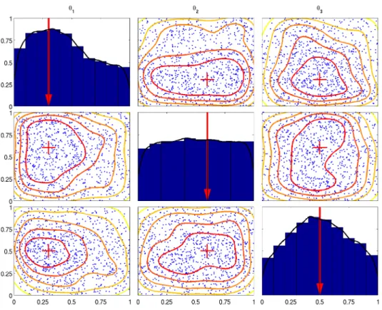
$,2px2q. Furthermore, we assess inference on the calibration parameters. In Figure 3.5, we observe that in most of the cases, the marginal posterior distribution densities of the calibration parameters are unimodal and mainly concentrated above areas around the corresponding ideal values. In Figure 3.6, we plot the output of the computer model mixture (weighted and calibrated according to the proposed method), the output of single computer models (calibrated by the BSMC method), and the output of the real system without noise. We used MAP estimates for the calibration parameters. We observe that the calibrated computer model mixture, fitted by the proposed method, successfully represents the real system, while the single models calibrated by the BSMC method fail. Therefore, the proposed method can successfully address problems where there are available multiple computer models with unknown fidelity order and there is need to accurately simulate the real system.

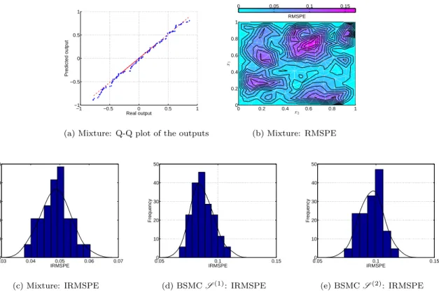
We examine the predictive ability of the proposed method. As performance measures, we consider the root mean squared predictive error (RMSPE)3_{, and the integrated RMSPE (IRMSPE)}4_{. In Figure 3.7a, we} observe that the predictions produced by the proposed method are close to the output values generated by the real system at the same input points. Moreover, we observe that the produced RMSPE in Figure 3.7b has small values throughout the input space. Hence, the proposed method can predict the output of the real system adequately. We compare the predictive ability of the proposed method with that of the standard Bayesian single model calibration (BSMC) procedure of Kennedy and O’Hagan [1] with respect to the IRMSPE. In Figures 3.7c-3.7e, the histograms of the IRMSPE values were generated based on 32

3_{RMSPEpxq “}b1

N

řN

i“1pζˆipxq ´ypxqq2 computed based onN generated training data-sets

4_IRMSPE“ 1

CardpX_gridq

ř

0 0.5 1 0 0.5 1 0 0.2 0.4 0.6 0.8 x₁ $₂₍x₎ x2 0.3 0.35 0.4 0.45 0.5 0.55 0.6 0.65 0.7

(a) Exact weight function$2p¨q

0 0.5 1 0 0.5 1 0 0.2 0.4 0.6 0.8 x₁ $₂₍x₎ x2 $ 2 ( x ) 0.3 0.35 0.4 0.45 0.5 0.55 0.6 0.65 0.7

(b) Est. weight function$2p¨q

−0.1 −0.05 0 0.05 0.1 0.15 0 10 20 Pr 0 2000 4000Iteration6000 8000 10000 b ia s( ˆ $ 2 ) (c) Bias of integrated$ˆ2p¨q 0 0.2 0.4 0.6 0.8 1 h(1) $,1(x1, x2) = 1 h(1) $,2(x1, x2) =−1 + 2·x1 h(1) $,3(x1, x2) =−1 + 2·x2

Marginal posterior inclusion probabilities

Legendre bases

Prob.

(d) Inclusion probabilities of the basesthp$,a1q u

Figure 3.4: (a): Exact weight function$2pxq “ p1`expp1´2x2qq´1 presented by colored surface. (b): Estimated

weight function$ˆ2p¨q “1´$ˆ1p¨qpresented by colored surface and95% credible intervals presented by red bars. (c):

Ergodic estimate of bias of integrated$2p¨qbiasp$2pXqq “ $ˆ2pXq ´$2pXq. (d): Frequency that each basis was

included in the weight function$p¨qas significant. (Section 3.2)

realizations of the training data and fitting the predictive model. In Figure 3.7c-3.7e, we observe that it is more likely for the proposed method to produce smaller IRMSPE than the BSMC method. This suggests that, the proposed method provides more accurate predictions than the BSMC, when multiple computer models with unknown fidelity order are available.

3.3. Application to large-scale climate modeling

Set-up of the application and computer models . We consider the Advanced Research Weather Research and Forecasting Version 3.2.1 (WRF Version 3.2.1) climate model [12] constrained in the geographical domain 25˝_–44˝_{N and112}˝_–90˝_{W over the Southern Great Plains (SGP) region, and we concentrate on the average}

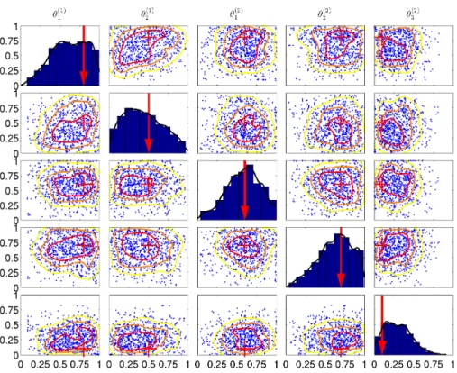
Figure 3.5: Estimated marginal posterior distribution densities of the calibration parameters. The ‘ideal’ values of the parameters are pointed by red arrows and red crosses. (Section 3.2)

monthly precipitation response. WRF is employed with the Kain-Fritsch convective parametrisation scheme (KF CPS) [16] as in [45]. The KF CPS is a simple 1D mass flux cloud model specifically designed for mesoscale models [16], including WRF, with a moderate grid spacing 10km-100km. The 5 most critical parameters [45] of the KF scheme are: the coefficient related to downdraft mass flux ratePdthat takes values in range r´1,1s; the coefficient related to entrainment mass flux rate Pe that takes values in ranger´1,1s; the maximum turbulent kinetic energy in sub-cloud layer (m2s´2_)P

t that takes values in ranger3,12s; the starting height of downdraft above updraft source layer (hPa)Phthat takes values in ranger50,350s; and the average consumption time of convective available potential energyPc that takes values in ranger900,7200s. The ranges of the KF CPS parameters are quite wide and hence cause higher uncertainties in climate simulations due to the non linear interactions and compensating errors of the parameters [46, 47, 45]. Other specifications used are the Morrison2-moment cloud microphysics scheme [48], the Noah land surface model [49], and the Mellor-Yamada-Janjic [50] planetary boundary layer turbulence scheme. Here, we consider two different radiation schemes, the Rapid Radiative Transfer Model (RRTMG) for General Circulation Models [51], and the Community Atmosphere Model 3.0 (CAM) [14]. Moreover, we consider two grid spacing,25km and 50km spacing, referring to the horizontal resolutions. Here, higher grid spacing does not necessarily

0 0.5 1 0 0.5 1 −1 −0.5 0 0.5 1 x₁ x₂ ζ ( x ) −0.6 −0.4 −0.2 0 0.2 0.4 0.6 0.8 (a)Z: Output 0 0.5 1 0 0.5 1 −1 −0.5 0 0.5 1 x₁ x₂ Output −0.6 −0.4 −0.2 0 0.2 0.4 0.6 0.8 (b) Mixture: Output 0 0.5 1 0 0.5 1 −0.5 0 0.5 1 1.5 x₁ x₂ Output 0 0.5 1 1.5 (c)Sp1q_{: Output} 0 0.5 1 0 0.5 1 −1.5 −1 −0.5 0 0.5 x₁ x₂ Output −1.5 −1 −0.5 0 (d)Sp2q_{: Output}

Figure 3.6: Output functions of the: (a) real system, (b) the computer mixture model weighted and calibrated with the proposed method, (c) theSp1q _{calibrated by BSMC, and (d) theS}p2q _{calibrated by BSMC. (Section 3.2)} lead to more accurate simulations with respect to the precipitation because WRF performance is sensitive to other physical parametrizations which is uncertain how they are affected to the grid spacing.

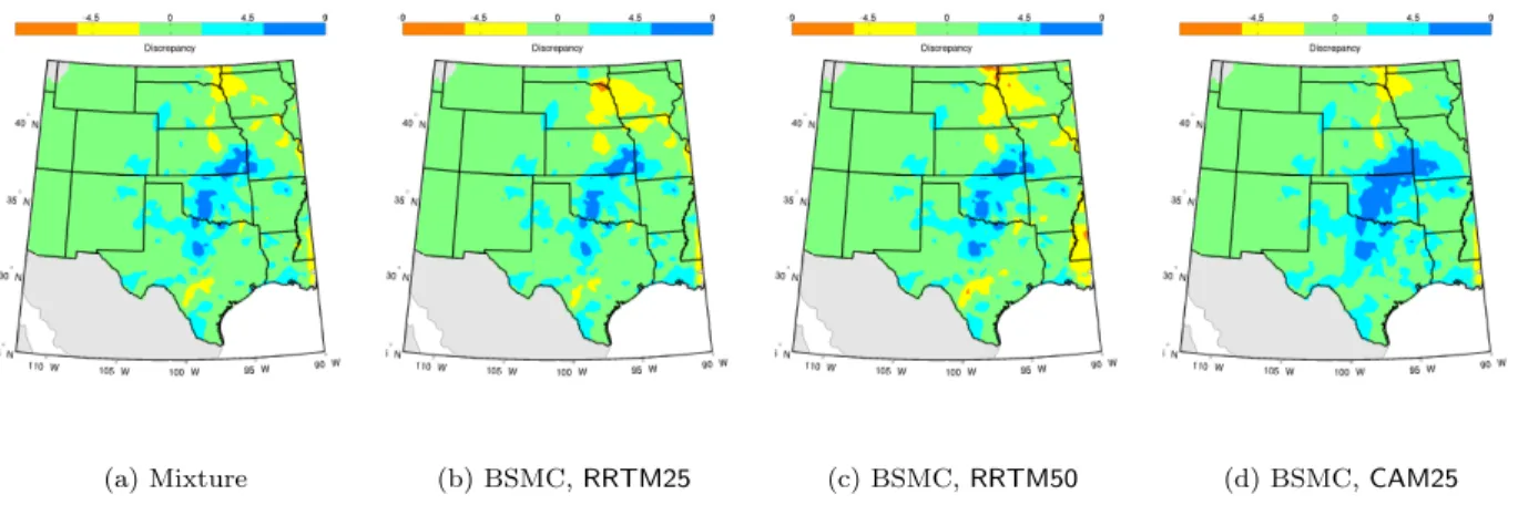
The available computer models are three different sub-models of the WRF with physics and fidelity variations. The first model involves the RRTMG radiation scheme with 25km horizontal grid spacing and 36 sigma levels from the surface to 1000hPa, and is labeled as RRTMG25; the second model involves the RRTMG radiation scheme with50km grid spacing, and is labeled asRRTMG50; and the third one involves the CAM 3.0 radiation scheme with25km grid spacing, and is labeled asCAM25. The output is the monthly average precipitation, the calibration parameters are the parameters of KF CPS, and the input are the coordinates in SGP.

Interest lies in combining properly the above computer models and hence their unique features; which allows to integrate both physics and fidelity variations. The reason is that aggregation of physics variability is expected to result in better prediction in climate models [15]. E.g., Yang et al. [45] observed that RRTMG radiation scheme tends to overestimate precipitation, while CAM tends to underestimate precipitation, given the default calibration values. An inexpensive but accurate surrogate model is of great interest because WRF requires several days to run. Also, it is of great interest to quantify the uncertainty ranges and identify the

−1 −0.5 0 0.5 1 −1 −0.5 0 0.5 1 Real output Predicted output

(a) Mixture: Q-Q plot of the outputs

0 0.2 0.4 0.6 0.8 1 0 0.2 0.4 0.6 0.8 1 x₂ x1 RMSPE 0 0.05 0.1 0.15 (b) Mixture: RMSPE 0.030 0.04 0.05 0.06 0.07 20 40 60 80 100 IRMSPE Frequency (c) Mixture: IRMSPE 0.050 0.1 0.15 10 20 30 40 50 IRMSPE Frequency (d) BSMCSp1q_{: IRMSPE} 0.050 0.1 0.15 10 20 30 40 50 IRMSPE Frequency (e) BSMCSp2q_{: IRMSPE}

Figure 3.7: (a): The Q-Q plot presents the predicted output of the surrogate model against the real output of the real system. (b): The contour plots present the RMSPEs as functions of the input parameterxPX, and (c-e): the histograms represent the distribution of the IRMSPEs, generated based on32realizations of the training data and fitting the predictive model. Procedures under comparison: the proposed method (Mixture), and BSMC method. (Section 3.2)

optimal values of the five key calibration parameters in the KF CPS used in WRF. Here, the calibration parameters have the same physical interpretation, however they may depend on the grid spacing. Therefore, it is of interest to conduct joint inference on these parameters across the modelsRRTMG25andCAM25, and separately by the modelRRTMG50.

Training data. Experimental data consist of 404 measurements from stations in the geographical domain 25˝_–44˝_{N and 112}˝_–90˝_{W over the SGP region, and represent monthly average precipitation (in mm) in}

June2007. The dataset is available from the U.S. Historical Climatological Network repository5 _[52]. Computer simulations were conducted over the same region by running the computer models: RRTMG25,

CAM25, and RRTMG50 with specific configurations. The designs of RRTMG25, CAM25, and RRTMG50,

consist of 50 simulations at different sets of calibration parameter values for each model, as well as at

4848, 4848, and 1211 coordinates on 25km, 25km, and 50km grid spacing correspondingly. Briefly, WRF simulations for each computer model were driven by the32km North American Regional Reanalysis (NARR), and lateral boundary conditions were updated every 3 hours. The first simulation was initialized on May 1st, 2007 and run for 1 month with the standard KF scheme until June 1st. Afterwords, all generated ensembles ran for another month through June2007, using identical initial land surface conditions from the first simulation on June1st. Atmospheric conditions were reinitialized by using the NARR data every2days in all simulations in order to minimize the potential effects of error in the simulated large-scale circulation and isolate the impact of convective parametrisation scheme on precipitation. Each simulation was run for3 days, but the first day was discarded as model spin-up. Since we are interested in the averaged precipitation, all the ensembles were averaged out with respect to the time. Therefore our analysis represents an average of15two-day ensembles (totaling1 month).

The validation data-set in order for us to assess the performance of the method consist of the post-processed University of Washington1{8 gridded precipitation data [53] which are very accurate.

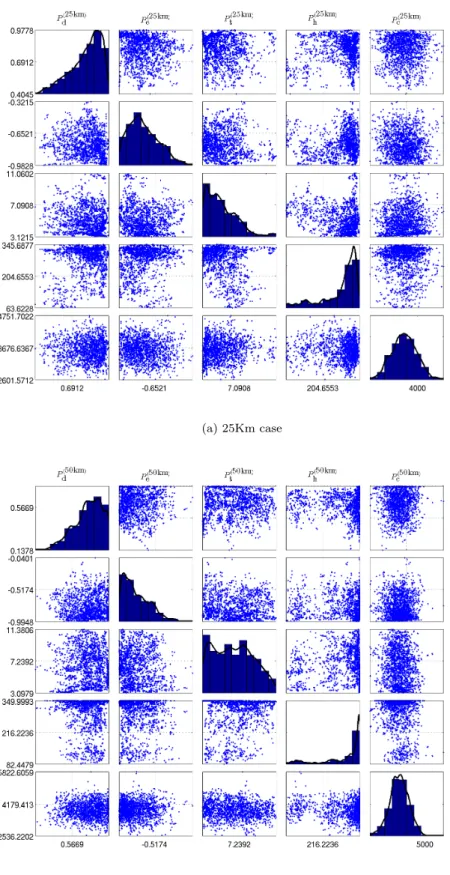
Uncertainty quantification analysis. We consider the proposed Bayesian calibration computer model mixture set-up with non informative priors. We transformed the precipitation values to the log scale to compensate for the positive values. The means of the Gaussian process priors assigned on the computer models output functions are modeled as2nd degree multivariate Legendre polynomial bases expansions, while that of the dis-crepancy function is modeled as a constant. Because the application involves a large data-set, we tapered the covariance functions by using the Wendland-1tapering function [54, 33, Chapter 9]. Through try-and-error runs, we found that an acceptable value for the tapering parameterγWis0.1of the range, that do not cause significant loss in the explanation of the variability. The reason is because small scale variabilities can be modeled by the compactly supported covariance function, while the larger scale variabilities can be explained by the bases expansion in the linear term of the Gaussian process [55, 56]. Regarding the weight functions, we considered a pool of2nd degree multivariate Legendre polynomial bases. We consider shared calibration parameters for computer modelsRRTMG25andCAM25aspP_dp25kmq, Pep25kmq, Pp

25kmq t , P p25kmq h , P p25kmq c q, and separate ones for computer modelsRRTMG50 as pP_dp50kmq, Pep50kmq, Pp

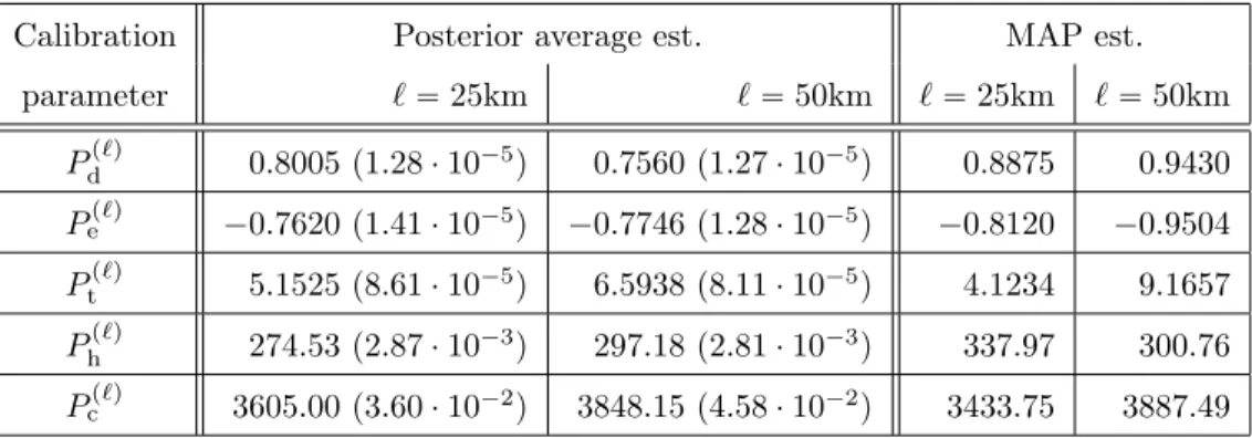
50kmq t , P p50kmq h , P p50kmq c q. On the cali-bration parameters, we assign independent truncated normal prior distributions whose hyper-parameters are specified through moment matching; and precisely by setting the prior means equal to the empir-ical values of the KF CPS scheme [45], and variances equal to the squared ranges. Namely, P_dp`q „ trNp5.5¨10´9<sub>,122.37</sub>2 q,Pep`q„trNp5.5¨10´9,122.372q,Pp `q t „trNp6.25,507.682q,P p`q h „trNp175,1.43 2 ¨1012q, and Pcp`q „trNp3.37e`3,7.232¨1012q, for` “25km,50km. For comparison reasons, we consider the tra-ditional Bayesian single model calibration of Higdon et al. [2] using the same specifications. The MCMC samplers ran for20000iterations where the first 10000where discarded as burn in.

(a)$RRTMG25p¨q (b)$RRTMG50p¨q (c)$CAM25p¨q 0 0.2 0.4 0.6 0.8 1 0 2 4 Pr 0 Iteration5000 10000 $ R R T M G 25 (d)$RRTMG25pX25kmq 0 0.2 0.4 0.6 0.8 1 0 2 4 Pr 0 Iteration5000 10000 $ R R T M G 50 (e)$RRTMG50pX25kmq 0 0.2 0.4 0.6 0.8 1 0 5 10 Pr 0 Iteration5000 10000 $ C A M 25 (f)$CAM25pX25kmq

Figure 3.8: (a-c): Estimate of the posterior weight function t$kp¨q;k “ RRTMG25,RRTMG50,CAM25u. (d-f):

Histograms and trace plots of the integrated posterior weightst$kpX25kmqcomputer on a25km space grid X25km.

Samples are generated by Algorithm 1. (Section 3.3)

Figures 3.8a, 3.8b, 3.8c, we observe that the RRTMG25 model tends to outperform the other two models in most of the regions while CAM25 tends to outperform the other two models around the areas of South Dakota and Nebraska, in terms of the representation of the precipitation. The overall contribution of the computer models in the mixture is indicated by the a posteriori integrated weight functions (Figures 3.8d, 3.8e, 3.8f). We observe that the posterior density of$RRTMG25pXqis over larger values than the others and without any significant overlapping, which indicates that, overally, RRTMG25 outperforms the other two. The associated trace plots suggest that the MCMC mixing was acceptable.

It is important to better understand the parameters of KF-CPS and constraint their ranges for future studies. Figure 3.9 presents histogram estimates of marginal calibration parameter posterior densities, and scatter plots of the generated calibration parameter values. We observe that the calibration parameter posteriors, in the two grid spacing cases25km and50km, do not differ significantly, with the only exception of Pt. Moreover, we observe that the posterior densities of KF-CPS parameters are concentrated around