Simulation-Based Finite-Sample Inference in Simultaneous
Equations
Jean-Marie Dufour
∗Université de Montréal
Lynda Khalaf
†Université Laval
December 8, 2003
∗
Centre Interuniversitaire de recherche en économie quantitative(CIREQ),Centre interuniversitaire de recherche en analyse des organisations(CIRANO), and Département de sciences économiques, Université de Montréal. Mailing address: C.R.D.E, Université de Montréal, C.P. 6128 succursale Centre Ville, Montréal, Québec, Canada H3C 3J7. TEL: (514) 343 2400; FAX: (514) 343 5831; e-mail: [email protected].
†Département d’économique andGroupe de Recherche en économie de l’énergie de l’environement et des ressources naturelles(GREEN), Université Laval, andCentre Interuniversitaire de recherche en économie quantitative(CIREQ), Université de Montréal. Mailing address: GREEN, Université Laval, Pavillon J.-A.-De Sève, St. Foy, Québec, Canada, G1K 7P4. TEL: (418) 656 2131-2409; FAX: (418) 656 7412; email: [email protected]
ABSTRACT
In simultaneous equation (SE) contexts, nuisance parameter, weak instruments and identifica-tion problems severely complicate exact and asymptotic tests (except for very specific hypotheses). In this paper, we propose exact likelihood based tests for possibly nonlinear hypotheses on the co-efficients of SE systems. We discuss a number of bounds tests and Monte Carlo simulation based tests. The latter involves maximizing a randomizedp-value function over the relevant nuisance pa-rameter space which is done numerically by using a simulated annealing algorithm. We consider limited and full information models. We extend, to non-Gaussian contexts, the bound given in Dufour (Econometrica, 1997) on the null distribution of the LR criterion, associated with possibly non-linear- hypotheses on the coefficients of one Gaussian structural equation. We also propose a tighter bound which will hold: (i) for the limited information (LI) Gaussian hypothesis consid-ered in Dufour (1997) and for more general, possibly cross-equation restrictions in a non-Gaussian multi-equation SE system. For the specific hypothesis which sets the value of the full vector of en-dogenous variables coefficients in a limited information framework, we extend the Anderson-Rubin test to the non-Gaussian framework. We also show that Wang and Zivot’s (Econometrica, 1998) asymptotic bounds-test may be seen as an asymptotic version of the bound we propose here. In addition, we introduce a multi-equation Anderson-Rubin-type test. Illustrative Monte Carlo experi-ments show that: (i) bootstrapping standard instrumental variable (IV) based criteria fails to achieve size control, especially (but not exclusively) under near non-identification conditions, and (ii) the tests based on IV estimates do not appear to be boundedly pivotal and so no size-correction may be feasible. By contrast, likelihood ratio based tests work well in the experiments performed.
Contents
1. Introduction 1
2. Framework 4
3. Pivotal Statistics in systems and subsystems 7
3.1. Non-Gaussian extensions of the Anderson-Rubin test . . . 7
3.2. Multi-equation non-Gaussian extensions of the Anderson-Rubin test . . . 12
3.3. Pivots in full systems . . . 15
4. General Hypotheses tests on structural coefficients 18 4.1. The full system approach . . . 18
4.2. The LI context . . . 20
5. Simulation based pivotal and bounds tests 23 6. A Simulation study 24 7. Conclusion 26
List of Assumptions, Propositions and Theorems
3.1 Theorem :Distribution of the AR test statistic . . . 83.2 Theorem :Distribution of the AR multivariate test . . . 13
3.3 Theorem :Characterization of Pivotal Statistics . . . 16
3.4 Theorem :Pivotal Statistics: a special case . . . 17
4.1 Theorem :Boundeldy Pivotal Statistics . . . 19
4.2 Theorem :Boundeldy Pivotal Statistics: a special case . . . 20
4.3 Theorem :Boundeldy Pivotal LI Statistics: a special case . . . 21
4.4 Theorem :Boundedly pivotal LI statistics . . . 22
List of Tables
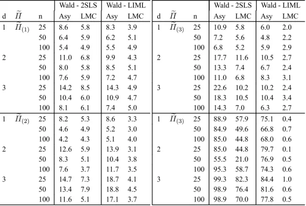
1 Empirical P(Type I error): Testing a subset of endogenous variables coefficients, LR tests. . . 272 Empirical P(Type I error): Testing a subset of endogenous variables coefficients, Wald tests. . . 28
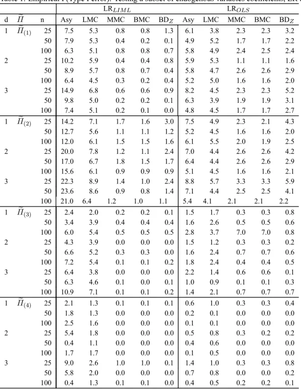
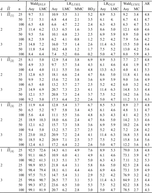
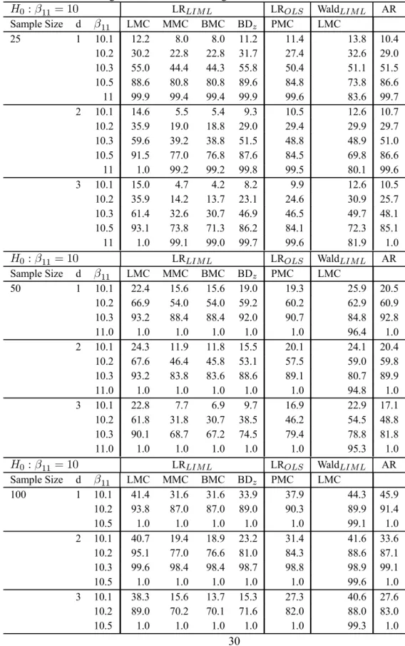
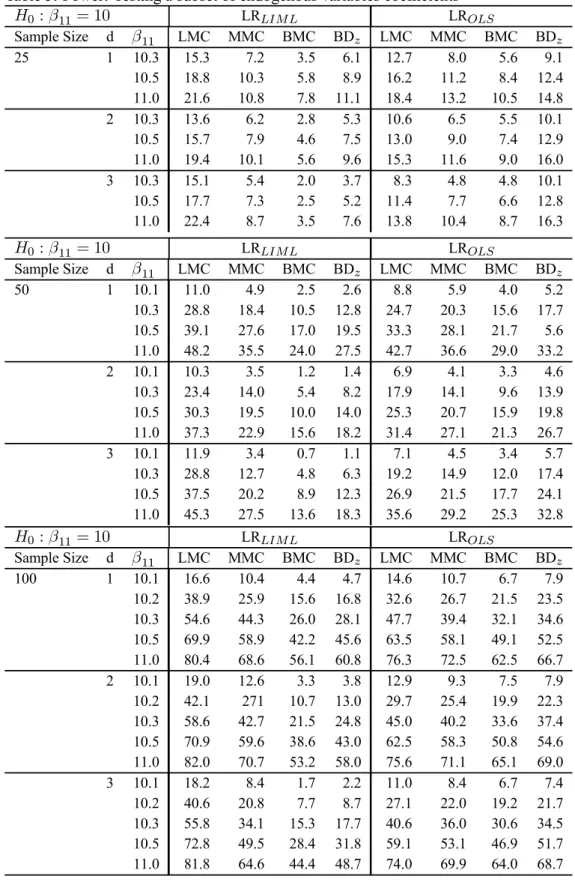
3 Empirical P(Type I error): Testing the full vector of endogenous variables coefficients 29 4 Power: Testing the full vector of endogenous variables coefficients . . . 30
1. Introduction
Hypotheses tests in simultaneous equation (SE) models are among the most enduring problems in econometrics. With few exceptions, the distributions of standard test statistics are known only asymptotically due to feedback from the dependent variables to the explanatory variables. Indeed, exact procedures have been proposed only for a few highly special cases. Early in the development of econometric theory relating to the SE model, Haavelmo (1947) constructed exact confidence re-gions for OLS reduced form parameter estimates and corresponding structural parameter estimates. Bartlett (1948) and Anderson and Rubin (1949, (AR)) proposed exactF-tests for specific classes
of hypotheses in the context of a structural equation along with corresponding confidence sets; see also Maddala (1974). Promising extensions of the AR test have recently been discussed in Dufour and Jasiak (2001), Dufour and Taamouti (2003c, 2003b, 2003a) and Dufour (2003). Some exact specification tests have also been suggested for SE. In particular, Durbin (1957) proposed a bounds test against serial correlation in SE and Harvey and Phillips (1980, 1981a, 1981b, 1989) have sug-gested tests against serial correlation, heteroskedasticity and structural change in a single structural equation; these tests are based on residuals from a regression of the estimated endogenous part of an equation on all exogenous variables. An exactF-test involving reduced form residuals was
pro-posed by Dufour (1987, Section 3), for the hypothesis of independence between the full vector of stochastic explanatory variables and the disturbance term of a structural equation.1 Beside these exceptions, available and routinely applied inference procedures in SE are asymptotic. In particular, instrumental variable (IV) methods are the most widely used in empirical practice.
The finite sample distributions of standard estimators and test statistics have received atten-tion early on in this literature. Initial studies (for surveys, see Phillips (1983) and Taylor (1983)) have revealed that: (i) exact distributions are highly complex; (ii) nuisance parameter problems severely hinder the development of exact tests (except for very specific hypotheses); (ii) asymptotic distributions may provide poor approximations in several cases. However, the severity of these find-ings and their implications on applied work were not recognized until the recent research on
near-identificationorweak instruments. Published papers dealing with such problems include: Nelson
and Startz (1990a), Nelson and Startz (1990b), Buse (1992), Choi and Phillips (1992), Maddala and Jeong (1992), Angrist and Krueger (1994), McManus, Nankervis and Savin (1994), Bound, Jaeger and Baker (1995), Cragg and Donald (1996), Hall, Rudebusch and Wilcox (1996), Dufour (1997), Shea (1997), Staiger and Stock (1997), Wang and Zivot (1998), Zivot, Startz and Nelson (1998), Stock and Wright (2000), Dufour and Jasiak (2001), Hahn and Hausman (2002, 2003), Kleibergen (2002), Moreira (2003a, 2003b), Stock, Wright and Yogo (2002), Kleibergen and Zivot (2003), Perron (2003), Wright (2003); several recent working papers are also cited in Dufour (2003) and Stock et al. (2002). Studies on weak instruments convincingly demonstrate that standard asymptotic procedures (i.e. procedure whichimpose identification awaywithout correcting for local-almost-identification (LAU)) are fundamentallyflowed and lead to serious overrejections; these problems are not small sample related and occur with fairly large sample sizes, since they are caused by asymptotics failures. In particular Dufour (1997) shows that usualt-type tests, based on common
IV estimators, have significance levels that may deviate arbitrarily from their nominal levels since 1This procedure generalizes earlier tests suggested by Wu (1973) and Hausman (1978)
it is not possible to bound their null distributions.
To circumvent weak-instruments related difficulties, the above cited recent work on SE has focused on three main directions (see the surveys of Dufour (2003) and Stock et al. (2002)): (i) refinements in asymptotic analysis which include the local-to-zero or local-to-unity frameworks (e.g. Staiger and Stock (1997), Wang and Zivot (1998)), (ii) asymptotic approximations which hold whether instruments are weak or not (e.g. Kleibergen (2002), Moreira (2003b)), and (iii) new finite-sample-justified procedures based on proper pivots, i.e. statistics whose null distributions are either nuisance parameter free or bounded by nuisance parameter free distribution [i.e. are boundedly
pivotal], (e.g. Dufour (1997), Dufour and Jasiak (2001), Dufour and Khalaf (2002), Dufour and
Taamouti (2003c, 2003b, 2003a)). So far, provably exact procedures are still in short supply, and typically require normal errors.
With the declining cost of computing, a natural alternative to traditional inference are simulation-based methods such as bootstrapping; for reviews, see Efron (1982), Efron and Tib-shirani (1993), Hall (1992), Jeong and Maddala (1993), Vinod (1993), Shao and Tu (1995), Li and Maddala (1996). These surveys suggest that bootstrapping can provide more reliable inference for many problems. In connection with the SE model, examples in which the bootstrap outperforms conventional asymptotics include: Freedman and Peters (1984a), Green, Hahn and Rocke (1987), Hu, Lau, Fung and Ulveling (1986), Korajczyk (1985), Dagget and Freedman (1985), and Mor-eira and Rothenberg (2003). Others however,find that the method leads to little improvement,e.g. Freedman and Peters (1984b), Park (1985) and Beran and Srivastava (1985), Moreira and Rothen-berg (2003). Clearly, there appears to be a conflict in the conclusions regarding the effectiveness of the bootstrap in SE contexts.2
This paper addresses these issues and develops alternative simulation based test procedures in limited and full information SE models. The tests we propose are motivated byfinite sample arguments. We focus on likelihood ratio (LR) based statistics. This choice is motivated by the propositions in Dufour (1997) pertaining to LR’sboundedly pivotalcharacteristic,i.e. the fact that LR admits nuisance-parameter-free bounds. Our contributions can be classified infive categories.
First, we extend, tonon-Gaussiancontexts, the bound given in Dufour (1997, (Theorem 5.1))
on the null distribution of the LR criterion, associated with possibly non-linear- hypotheses on the coefficients ofoneGaussian structural equation.3We also propose a tighter bound which will hold: (i) for the limited information (LI) Gaussian hypothesis considered in Dufour (1997, (Theorem 5.1)) (i.e. in the context of the LR statistic based on limited information maximum likelihood (LIML) estimation), and (ii) for more general, possibly cross-equation restrictions in a non-Gaussian multiequation SE system. Formally, we show that Dufour (1997)’s result may be obtained as a special -although non-optimal - case of our proposed bound. To do this, we use the results of Dufour and Khalaf (2002) on hypotheses tests in multivariate linear regression (MLR) models.4
2In fact, it is well known that bootstrapping may fail to achieve size control when the asymptotic distribution of the underlying test statistic involves nuisance parameters [see Athreya (1987), Basawa, Mallik, McCormick, Reeves and Taylor (1991) and Sriram (1994), and Dufour (2002).
3SE LR tests often involve non-linear hypotheses implied by the structure; in connection, see Bekker and Dijkstra (1990) or Byron (1974)
4The relationship between the MLR and the SE model is readily seen: when all the predetermined variables of a SE system are strictly exogenous, the reduced form is equivalent to a (restricted) MLR system.
Second, for the specific hypothesis which sets the value of the full vector of endogenous vari-ables coefficients in a LI framework, we show that Wang and Zivot (1998)’s asymptotic bounds-test may be seen as an asymptotic version of the bound we propose here. We use this result to extend the validity of Wang and Zivot (1998)’s bound to the case of general linear hypotheses on structural coefficients. To do this, we show that our general bound on the LIML is based on an AR-type bounding pivotal statistic.
Third,we extend the AR-test to the non-Gaussian framework. Specifically, we show analytically
that the proof of its pivotality infinite samplesdoes not require normal errors. This is achieved by re-writing the AR statistic as an LR-type criterion (based on the LI reduced form). To date, available exact AR-type tests require normality assumptions. In this regard, our results are noteworthy.
Fourth, our re-interpretation of the AR-test allows to re-write Kleibergen (2002)’s test as a
approximate generalized AR-test (see Dufour (2003) and Dufour and Taamouti (2003c, 2003b, 2003a)) obtained with a specific instrument substitution choice. Specifically, we prove analytically that Kleibergen (2002)’s test can be obtained as an F-test for the exclusion of a specific instrument matrix, based on a constrained estimate of the coefficient of the excluded regressors in thefirst stage regression. To do this, we use the expression provided in Dufour (2003, Section 6.3 (d)) as well as known results from the MLR literature (Berndt and Savin (1977), Dufour and Khalaf (2002)).
Fifth, we propose a multi-equation Anderson-Rubin-type test which also admits a pivotal bound
based on the results of Dufour and Khalaf (2003) relating to SURE models. In view of the renewed interest in the Anderson-Rubin test (see Dufour (1997), Dufour and Jasiak (2001), Staiger and Stock (1997), Wang and Zivot (1998) and Dufour and Taamouti(2003c, 2003b, 2003a)), extensions to a systems context may prove useful.
It is important, at this stage, to emphasize that the distributional theory which underlies all the above procedures holds whether identification constraints are imposed or not. Consequently, identification problems are resolved without the need to introduce non-standard, e.g. local-to-zero, asymptotics. Furthermore, although exactness is obtained under parametric assumptions (which are duly defined in the paper), normality is not strictly required.
Sixth, this paper makes several contributions relevant to simulation-based tests. Indeed, the
null distribution of all statistics considered may be quite complex, particularly in non-Gaussian contexts. In view of this, we propose, following Dufour and Khalaf (2002), to apply the Monte Carlo (MC) test procedure [Dwass (1957), Barnard (1963), Dufour (2002)] to obtain simulation based exact p-values. MC test procedures may be viewed as parametric bootstrap tests applied to statistics whose null distribution does not involve nuisance parameters, with however a fundamental additional observation: the associated randomized test procedure can easily be performed to control test size exactly, for a given number of replications.
Here, recall that we consider two types of statistics, the pivotal ones (our extensions of the AR test), and the boundedly pivotal ones (general LR-LIML and multi-equation AR test). The MC test method easily yields exact p-values given pivotal statistics; to avoid confusion in what follows, we will refer to MC tests based on exact pivots aspivotal MC tests(PMC). Boundedly pivotal statis-tics are approached through two MC test procedures. First, we consider thebounds-MC technique
(BMC) (Dufour (2002), Dufour and Khalaf (2002)). This methods differs from the PMC one in the fact that the null distribution of the bounding statistics (which is pivotal by construction) is
consid-ered. Second, we apply themaximized MC method(MMC) (Dufour (2002)); this method requires; (i) defining a p-value function which gives a bootstrap-type MC p-value conditional on relevant nui-sance parameters, (ii) maximizing the latter function (using global maximization algorithms) over these nuisance parameters.5 The latter method may be viewed as a numerical search for the optimal bound.
It is clear that such a search may be computationally expensive. So we propose to combine the BMC with an MMC test, which can be run whenever the bounds test is not significant. To understand this strategy, recall that the BMC test is exact in the sense that rejections (at levelα) are
conclusive. Furthermore, we show that the MMC algorithm may be written in a way to include a standard parametric bootstrap as afirst step. Possibly expensive iterations - to obtain the maximal MC p-value in question which underlies the MMC test - may thus be saved if the bootstrap p-value exceedsα.
To illustrate the performance of these tests particularly given identification issues, we run a small-scale simulation experiment. Our mainfindings are: (i) MC methods based on randomization procedures where unknown parameters are replaced by estimators do not achieve size control, and (ii) MMC p-values for IV-based test are always one; in other words, it is does not appear possible tofind a non trivial bound on the rejection probabilities, so that standard asymptotic and bootstrap procedures are deemed to fail when applied to such statistics. In contrast, LR-based MMC tests allow one to control the level of the procedure.
The paper is organized as follows. Section 2 develops the notation and definitions. In Section 3 we discuss pivotal statistics in full and sub-systems; general hypotheses are considered in Section 4. The MC test procedures applied to pivotal and general hypotheses are presented in 5. Simulation results are reported in Section 6 and Section 7 concludes the paper.
2. Framework
We consider a system ofpsimultaneous equations of the form
Y B+XΓ =U, (2.1)
whereY = [y1, ... , yp]is ann×p matrix of observations onpendogenous variables, Xis an
n×kmatrix offixed (or strictly exogenous) variables andU = [u1, ... , up] = [U1, ... , Un]0is a matrix of random disturbances. The coefficient matrixBis assumed to be invertible. The equations
in (2.1) give the structural form of the model. Post-multiplying both sides by B−1 leads to the reduced form
Y =XΠ+V, Π=−ΓB−1, π=vec(Π), (2.2)
whereV = [v1, ... , vp] = [V1 , ... , Vn]0 is the matrix of reduced form disturbances. Further, we suppose the rows ofU satisfy the following distributional assumptions:
Ut∼JWt, t= 1, ... , n, (2.3)
5MMCp-values are computed using a simulated annealing (SA) optimization algorithm; see Corana, Marchesi, Mar-tini and Ridella (1987) or Goffe, Ferrier and Rogers (1994).
where the vectorw=vec(W1, ... , Wn)has a known distribution andJis an unknown nonsingular matrix; for further reference, letW = [W1, ... , Wn]0 where (2.3) implies that
W =U(J−1)0. (2.4)
WhenV ar(Wt) =Ip,var(Ut) =JJ0 ≡Ωandvar(Vt) = (B−1)0ΩB−1= (B−1)0J J0B−1 ≡Σ. Of course, condition (2.3) will be satisfied when
Wt∼N(0, Ip), t= 1, ... , n. (2.5)
A key feature of SE models is the imposition of identification conditions on the structural coeffi-cients. Usually, these conditions are formulated in terms of zero restrictions onBandΓ.In addition,
a normalization constraint is imposed which is usually achieved by setting the diagonal elements of
Bequal to one. We can rewrite model (2.1), given exclusion and normalization restrictions as yi =Yiβi+X1iγ1i+ui, i= 1, ... , p, (2.6) whereYiandX1iaren×miandn×kimatrices which respectively contain the observations on the included endogenous and exogenous variables of the model. Many problems are also formulated in terms of limited-information (LI) models such as
yi =Yiβi+X1iγ1i+ui =Ziδi+ui,
Yi =X1iΠ1i+X2iΠ2i+Vi,
(2.7)
where Zi = [Yi, X1i], δi = (β0i,γ01i)0 andX2i refers to the excluded exogenous variables. The associated LI reduced form is
£ yi Yi ¤ = XΠi+ £ vi Vi ¤ , Πi = · π1i Π1i π2i Π2i ¸ , X=£ X1i X2i ¤ (2.8) π1i = Π1iβi+γ1i, π2i=Π2iβi, (2.9) which lead to the necessary and sufficient condition for identification
rank(Π2i) =mi. (2.10)
Our LI-analogue of (2.3) can be stated as follows. LetVitrefer to thetth row ofVi, then the rows of£ ui Vi
¤
satisfy the following distributional assumptions:
¡
uit Vit0 ¢∼JiWti, t= 1, ... , n, (2.11) where vec(W1i , ... , Wni) has a known distribution and Ji is an unknown non-singular matrix. WhenV ar(Wti) =Imi+1,
var¡ uit Vit0
¢
For further reference, letWi = [W1i, ... , Wni]0where (2.11) implies that
Wi =£ ui Vi
¤
(Ji−1)0. (2.13)
In this context, LIML corresponds to maximizing, imposing (2.9), the likelihood function
L(yi, Yi|X1i, X2i) =− n(m+ 1) 2 ln(2π)− n 2 ln|Σi|− 1 2trΣ −1 i D0iDi, (2.14) whereDi = £ yi Yi ¤
−XΠiandΣidenotes the relevant reduced form error covariance. Numer-ical maximization may be considered, yet it is well know that an equivalent solution obtains through an eigenvalue/eigenvector problem based on the following determinantal equation
¯ ¯ ¯£ yi Yi ¤0 M1i £ yi Yi ¤ −λi £ yi Yi ¤0 M£ yi Yi ¤¯¯¯= 0 (2.15) whereM =I−X(X0X)−1X0,M1i=I−X1i(X10iX1i)−1X10iandλi refers to the eigen value in question. Indeed, it can be shown (see, for example Davidson and MacKinnon (1993, Chapter 18), Wang and Zivot (1998)) that the estimator ofβisβei = ARGMIN
βi {λ(βi)} λ(βi) = [yi−Yiβi] 0M 1i[yi−Yiβi] [yi−Yiβi]0M1i(I−M1iX2i(X20iM1iX2)−1X20iM1i)M1i[yi−Yiβi] . (2.16)
Formally, the LIML estimator ofβiandγ1i is
e δi = · eβi e γ1i ¸ = · Yi0Yi−eλiYi0M Yi Yi0X X0Yi X0X ¸−1· Yi0−eλiYi0M Xi0 ¸ yi (2.17)
whereeλiis the smallest root of (2.15), which corresponds toλ(eβi)[whereλ(βi)is given by (2.16)]. Correspondingly, expressions for the reduced form parameter estimates obtain as follows (see Theil (1971), appendix B): h e π1i Πe1i i = (X10iX1i)−1X10i ³£ yi Yi ¤ −X2i h e π2i Πe2i i´ (2.18) h e π2i Πe2i i = (X20iM1iX2i)−1X20iM1i £ yi Yi ¤ (2.19) −(X 0 2iM1iX2i)−1X20iM1i £ yi Yi ¤ · 1 −eβi ¸0 e Σi · 1 −βei ¸ · 1 −eβi ¸ · 1 −eβi ¸0 e Σi e Σi = £ yi Yi ¤0M£ y i Yi ¤ n + (eλ−1) n (2.20)
× £ yi Yi ¤0 M£ yi Yi ¤· 1 −eβi ¸ µ£ yi Yi ¤0 M£ yi Yi ¤· 1 −eβi ¸¶0 · 1 −βei ¸0£ yi Yi ¤0 M£ yi Yi ¤· 1 −eβi ¸ .
The derivations of Theil (1971) also imply that¯¯¯ eΣi
¯ ¯ ¯satisfies ¯ ¯ ¯ eΣi ¯ ¯ ¯=eλi ¯ ¯ ¯0£ yi Yi ¤0M£ y i Yi ¤¯¯¯. (2.21)
For hypotheses of the formRiδi=rion the coefficients of (2.7), whereRi is a knownqi×mi matrix of rankqiandriis known, Wald statistics are routinely applied and take the form
τw = 1 s2(ri−Ribˆδi)0−[R0i(ZiPi(Pi0Pi)−1Pi0Zi)−1Ri] (ri−Ribˆδi), (2.22) s2 = 1 n(yi−Zi b ˆδi)0(y i−Zibˆδi)0
wherebˆδiis a consistent asymptotically normal estimator such as (2.17) or the 2SLS ˆ
δi= [Zi0Pi(Pi0Pi)−1Pi0Zi]−1Zi0Pi(Pi0Pi)−1Pi0yi, Pi= [ X X(X0X)−1X0Yi ].
Imposing identification, the asymptotic null distribution ofτw isχ2(q). For an asymptotic theory conformable with under-identification, see Staiger and Stock (1997).
3. Pivotal Statistics in systems and subsystems
The recent literature on SE models has underscored the importance of proper pivots. This section characterizes pivotal statistics in possibly non-Gaussian systems and subsystems, which include the case of one single structural equation (the LI case). Wefirst consider the LI context, since it is a fundamental one, and because it may be used to explicate our multi-equation approach.
3.1. Non-Gaussian extensions of the Anderson-Rubin test
In the context of the LI model (2.7), consider hypotheses of the form:
HAR:βi =β0i, (3.1)
whereβ0i is a known vector. Lety0i = yi−Yiβ0i; then (3.1) may be tested in the context of the transformed structural system
yi0 = Yi(βi−β0i) +X1iγ1i+ui, (3.2)
with reduced form £ y0 i Yi ¤ = £ X1i X2i ¤ Πi+ £ ui+V(βi−β0i) Vi ¤ , π1i = Π1i(βi−β0i) +γ1i, π2i =Π2i(βi−β0i). LetO(s,j)denotes a zeros×jmatrix. In this context, (3.1) corresponds to testing
£ O(k−ki, ki), I(k−ki) ¤ ΠiCi = 0, Ci = · 1 O(mi,1) ¸ . (3.4)
To simplify the presentation, note that since the hypothesis concerns solely the element ofβi, the
test may be recast in the context of:
M1i £ y0 i Yi ¤ Ci = M1iX2iΠAR+M1i £ ui+Vi(βi−β0i) Vi ¤ Ci ΠAR = £ π2i Π2i ¤ Ci
with null hypothesisΠAR = 0. The QLR statistic in this case takes the form (see Dufour and Khalaf (2002)) wherePM1iX2i =I −M1iX2i(X20iM1iX2i)−1X20iM1i |ΣˆAR0 | |ΣˆAR| = C 0 i £ y0 i Yi ¤0 M1i £ y0 i Yi ¤ Ci C0 i £ yi0 Yi ¤0M 1iPM1iX2iM1i £ y0i Yi ¤ Ci = y 00 i M1iyi0 y00 i M1iPM1iX2iM1iy 0 i which is a monotonic transformation of the Anderson-Rubin statistic.
Theorem 3.1 DISTRIBUTION OF THE ARTEST STATISTIC. In the context of the LI model(2.7),
consider the problem of testing(3.1)
HAR:βi=β0i
imposing(2.11)where thefirst row ofJihas zeros everywhere except for thefirst element. Let
ΛAR =
[yi−Yiβ0i]0M1i[yi−Yiβ0i]
[yi−Yiβ0i]0M1iPM1iX2iM1i[yi−Yiβ0i]
(3.5)
be the associated Anderson-Rubin statistic. Then under the null hypothesis P[ΛAR≥x] =P · |w0 iM1iwi| |wi0M1iPM1iX2iM1iwi| ≥x ¸ , ∀x, wherewi = ¡ wi 1 wi2 ... win
¢0 gives thefirst column of
Wias defined in(2.11)-(2.13).
PROOF.Under the null hypothesis,
|Σˆ0AR| |ΣˆAR| = u 0 iM1iui u0 iM1iPM1iX2iM1iui .
Given assumption (2.11), ui =
£
ui Vi
¤
Ci = WiJi0Ci. When the first row of Ji in (2.11) has zeros everywhere, except for the first element which equals σ 6= 0, then Ji0Ci = σCi and
WiJ0 iCi =σwi=σWiCi, so |Σˆ0 AR| |ΣˆAR| = σC 0 iWi0M1iWiCiσ σCi0Wi0M1iPM 1iX2iM1iM1iW iC iσ = C 0 iWi0M1iWiCi Ci0Wi0M1iPM 1iX2iM1iW iC i . (3.6)
Then the result obtains on observing thatwi =WiCi.¥
The latter result means that an exact test can be carried out in non-normal context without the need to specify the distribution of the full Wi matrix. If normality is further imposed, then it is
straightforward to see (see also Dufour and Khalaf (2002)) that
[ΛAR−1]
n−k k−ki ∼
F(k−ki, n−k).
As usual, the AR procedure can be adapted to test hypotheses onγ1i(in addition to constraints on βi). It is clear that our results will apply to this case as well. So consider now the problem of testing
HARX :βi=β0i, γ11i =γ011i (3.7) whereγ1i = (γ011i,γ012i),γ11iisk1i×1, andX1i = £ X11i X12i ¤ is decomposed conformably. The associated Anderson-Rubin statistic
ΛARX = £ yi−Yiβ0i−X11iγ011i ¤0M 12i £ yi−Yiβ0i−X11iγ011i ¤ £ yi−Yiβ0i−X11iγ011i ¤0M 12iPM12iX22iM12i £ yi−Yiβ0i−X11iγ011i ¤ M12i = I−X12i(X120 iX12i)−1X120 i, X22i = £ X11i X2i ¤ PM12iX22i = I−M12iX22i(X220 iM12iX22i)−1X220 iM12i.
Then following the same arguments as in Theorem3.1, we can show that under the null hypothesis
P[ΛARX ≥x] =P · |w0iM12iwi| |w0iM12iPM12iX22iM12iwi| ≥x ¸ ,∀x, (3.8)
and if normality is further imposed,
[ΛARX−1]
n−k k−ki−k1i ∼
F(k−ki−k1i, n−k). (3.9) Finally, consider the hypothesis analyzed in Dufour and Jasiak (2001, Section 4):
where Q1i is a q1i ×ki matrix whereq1i = rank(Q1i); Q1i can be treated as submatrix of an invertibleki×kimatrixQi= £ Q01i Q02i ¤0so that Qiγ1i= · Q1iγ11i Q2iγ21i ¸ = · ν1i ν2i ¸ . LetXQi = X1iQ− 1 i = £ XQ1i XQ2i ¤
whereXQ1i andXQ2i areT ×q1i andT ×(ki −q1i) matrices, so the LI equation can be re-written as
yi =Yiβi+XQ1iν1i+XQ2iν2i+ui,
in which case testingHARQX amounts to assessingβi =βi0, ν1i =ν0.The associated
Anderson-Rubin statistic ΛARQX = [yi−Yiβ0i−XQ1iν0] 0M Q2i[yi−Yiβ0i−XQ1iν0] [yi−Yiβ0i−XQ1iν0] 0M Q2iPMQ2iX22iMQ2i[yi−Yiβ0i−XQ1iν0] MQ2i = I−XQ2i(XQ0 2iXQ2i)− 1X0 Q2i, X22i= £ XQ1i X2i ¤ PMQ2iX22i = I−MQ2iX22i(X 0 22iMQ2iX22i) −1X0 22iMQ2i. The same arguments underlying (3.8) yield
P[ΛARQX≥x] =P ¯ |w0iMQ2iwi| ¯ ¯w0iMQ2iPMQ2iX22iMQ2iwi ¯ ¯ ¯ ≥ x ,∀x, (3.11)
and imposing normality
P[[ΛARQX−1]
n−k k−ki−q1i ≥
x] =P[F(k−ki−q1i, n−k)≥x]. (3.12) It is also easy to show, using the same arguments as in the above Theorems, that all the roots of the determinantal equation
¯ ¯ ¯yi00MQ2iy 0 i −µ y0i0MQ2iPMQ2iX22iMQ2iy 0 i ¯ ¯ ¯ = 0 [yi−Yiβ0i−XQ1iν0] = y 0 i
are pivotal under the null hypothesis, which lead to alternative statistics, such as the Lawley-Hotelling trace criterion, the Bartlett-Nanda-Pillai trace criterion and the maximum Root criterion.6 To conclude this section, it is useful to consider the test proposed by Kleibergen (2002) in the context of (3.1). Dufour (2003) shows that the latter test corresponds to an AR-type test applied with a specific instrument choice (denotedZK). Specifically, equations 83-86 from Dufour (2003)
rewritten in terms of the transformed model M1i £ yi Yi ¤ =M1iX2i £ π2i Π2i ¤ +M1i £ ui Vi ¤ (3.13) lead to the instrument
ZK = X2iΠ2i, Π2i=Πb2i−bπ2i(βei) SεV(β0i) Sεε(β0i) (3.14) b Π2i = (X20iM1iX2i)−1X20iM1iYi, bπ2(β0i) = (X20iM1iX2i)−1X20iM1i £ yi−Yiβ0i ¤ SεV ¡ β0i¢ = 1 T −k £ yi−Yiβ0i ¤0 M Yi, Sεε(β0i) = 1 T−k £ yi−Yiβ0i ¤0 M£yi−Yiβ0i ¤ .
Here we argue that the later expression is a constrained OLS estimator ofΠ2i, imposing the LIML structure. Expressions for constrained OLS estimates of (3.13) can be derived using the formulae from the general theory on MLR imposing uniform linear hypotheses (see Berndt and Savin (1977, equations 5 and 6) and Dufour and Khalaf (2002)). In is context, the AR null hypothesis takes the form (in the notation of Berndt and Savin (1977))F£ π2i Π2i
¤
G=E,whereF =Ik2,E = 0
andG=¡1,−β0i0¢0. Then applying equation (5) from Berndt and Savin (1977) which we reproduce
here for convenience (where P0 and P give the formula for the constrained and unconstrained
estimators of£ π2i Π2i ¤ in (3.13)) P0 = P − ³ e X0Xe´−1F0 · F³Xe0Xe´−1F0 ¸−1 (F P G−E)£G0SG¤−1G0S, P = ³Xe0Xe´−1Xey, Se = (ye−XPe 0)0(ye−XPe 0), e y = M1i £ yi Yi ¤ , Xe =M1iX2i,
yields the following expression for the constrained QMLE estimates:7
h b π02i Πb0 2i i = (X20iM1iX2i)−1X20iM1i £ yi Yi ¤ −(X 0 2iM1iX2i)−1X20iM1i £ yi Yi ¤ · 1 −β0i ¸0 b Σi · 1 −β0i ¸ · 1 −β0i ¸ · 1 −β0i ¸0 b Σi or alternatively h b π02 Πb20 i = (X20iM1iX2i)−1X20iM1i £ yi Yi ¤ −(X20iM1iX2i)−1X20iM1i £ yi−Yiβ0i ¤ £yi−Yiβ0i ¤0M£ y i Yi ¤ £ yi−Yiβ0i ¤0 M£yi−Yiβ0i ¤.
7A similar expression for the constrained LIML estimator ofΠ
Post-multiplying the latter expression by
·
O(1, m)
Im
¸
leads to the estimator
b Π20i =Πb2i−(X20iM1iX2i)−1X20iM1i £ yi−Yiβ0i ¤ £yi−Yiβ0i ¤0M Y i £ yi−Yiβ0i ¤0 M£yi−Yiβ0i ¤.
which is exactly equal toΠ2ias defined in (3.14). Recall that Dufour (2003) has shown that Wang and Zivot (1998)’s LMGM M test obtains as an AR-type test with instrumentX2iΠb2i. We thus see that Kleibergen (2002) is highly related to the latter, since it is obtained in a similar way, replacing the unconstrained OLS estimator ofΠ2i by a constrained OLS estimator which imposes the struc-ture. As mentioned in Dufour (2003), these tests are affected by the fact that instruments are not independent from the error termui, and thus are not pivotal infinite samples.
3.2. Multi-equation non-Gaussian extensions of the Anderson-Rubin test
The results of the previous section provide the basis for extending the AR procedure to multi-equation contexts. Consider a subset of thep-equation system (2.6),
yi =Yiβi+X1iγ1i+ui, i= 1, ... , m, (3.16) wherem≤p. In this context, consider the problem of testing,
HM AR:βi =β0i, i= 1, ..., m. (3.17)
Typically, when equations in (3.16) are viewed as a system, thefirst stage in an IV-type procedure consist in regressing each left-hand side endogenous variable on all the exogenous variables of the full sub-system. Conformably, letZ2refer to the set of exogenous variables that are excluded from
allmequations, so thatX=£ Z1 Z2
¤
; then thefirst stage regression corresponds to
Y =Z1Π1+Z2Π2+V , (3.18)
where Y includes all the distinct right-hand-side endogenous variables and the error term V is
defined conformably; suppose thatY isT ×mandZ1 isT ×k. By definition, postmultiplyingY
by a selection matrix (of zeros and ones) givesYi, which allows to decompose (3.18) as follows:
Yi=Z1Π1i+Z2Π2i+Vi, i= 1, ..., m,
whereViincludes the relevant columns ofV, andΠ1iandΠ2i are the relevant sub-matrices ofΠ1
andΠ2. Transform the system settingy0i =yi−Yiβ0i, i= 1, ..., m, as follows:
yi0 = Yi(βi−β0i) +Z1γi+ui (3.19)
whereγi may include zeros so thatZ1γi=X1iγ1i. This leads to the reduced form £ y10 ... ym0 Y ¤ = £ Z1 Z2 ¤· π11 ... π1m Π1 π21 ... π2m Π2 ¸ +£ u1+V1(β1−β01) ... um+Vm(βm−β0m) V ¤ , π1i = Π1i(βi−β0i) +γi, π2i=Π2i(βi−β0i), in which case (3.17) corresponds to testing:
h O(k−k, k), I(k−k)i · π11 ... π1m Π1 π21 ... π2m Π2 ¸ C = 0, C= · Im O(m, m) ¸ . (3.21)
These constraints do not consider the exclusions implied by the zeros in γi. Let MZ1 = I −Z1(Z10Z1)−1Z10 andΠAR =
£
π21 ... π2m Π2
¤
C. Then the test amounts to assessing
ΠAR= 0in the context of:
MZ1 £ y01 ... y0m Y ¤C = MZ1Z2ΠAR +MZ1 £ u1+V1(β1−β01) ... um+Vm(βm−β0m) V ¤ C LetPMZ 1Z2 =I−MZ1Z2(Z 0 2MZ1X2)− 1Z0
2MZ1, then the LR statistic to testΠAR= 0is
ΛMAR = ¯ ¯ ¯C0£ y0 1 ... ym0 Y ¤0M Z1 £ y0 1 ... ym0 Y ¤ C ¯ ¯ ¯ ¯ ¯ ¯C0£ y0 1 ... y0m Y ¤0M Z1PMZ 1Z2MZ1 £ y0 1 ... y0m Y ¤ C ¯ ¯ ¯ , = ¯ ¯ ¯£ y10 ... ym0 ¤0MZ1 £ y10 ... ym0 ¤¯¯¯ ¯ ¯ ¯£ y01 ... ym0 ¤0MZ1PMZ 1Z2MZ1 £ y01 ... ym0 ¤¯¯¯ .
Theorem 3.2 DISTRIBUTION OF THE ARMULTIVARIATE TEST. In the context of the subsystem
(3.16)of the SE model(2.1),consider the problem of testing(3.17)
HM AR:βi =β0i, i= 1, ..., m,
where, without loss of generality, them-equations under test are thefirstmequations of the system
so that £ u1 ... um ¤ =U C, C= · Im O(p−m, m) ¸
whereUsatisfies(2.3), with
J = · J11 0 J21 J22 ¸ , J11:m×m , J11is nonsingular (3.22)
andWis partitioned conformably as follows W = £ W1 W2 ¤ , Wi= [Wi1, . . . , WiT] 0 , i= 1,2, (3.23) Wt = · W1t W2t ¸ , W1t:m×1. Let ΛM AR = ¯ ¯ ¯£ y10 ... ym0 ¤0MZ1 £ y10 ... ym0 ¤¯¯¯ ¯ ¯ ¯£ y01 ... ym0 ¤0MZ1PMZ 1Z2MZ1 £ y01 ... y0m ¤¯¯¯ be the associated multivariate Anderson-Rubin statistic. Then under the null hypothesis
P[ΛM AR≥x] =P ¯ |W10MZ1W1| ¯ ¯W0 1MZ1PMZ1Z2MZ1W1 ¯ ¯ ¯ ≥ x , ∀x.
PROOF.Under the null hypothesis,
ΛM AR = ¯ ¯ ¯£ u1 ... um ¤0M Z1 £ u1 ... um ¤¯¯¯ ¯ ¯ ¯£ u1 ... um ¤0M Z1PMZ 1Z2MZ1 £ u1 ... um ¤¯¯¯ , £ u1 ... um ¤ = U C =W J0C=W · J110 0 ¸ =W1J 0 11.
SubstitutingW1J110 forU CinΛM ARleads to
ΛM AR = ¯ ¯ ¯J11W10MZ1W1J 0 11 ¯ ¯ ¯ ¯ ¯ ¯J11W10MZ1PMZ 1Z2MZ1W1J 0 11 ¯ ¯ ¯ = | J11| |W10MZ1W1| ¯ ¯ ¯J110 ¯¯¯ |J11| ¯ ¯ ¯W10MZ1PMZ 1Z2MZ1W1 ¯ ¯ ¯¯¯J110 ¯¯ = |W 0 1MZ1W1| ¯ ¯ ¯W10MZ1PMZ 1Z2MZ1W1 ¯ ¯ ¯ .
This completes the proof.¥
In this case as well, it easy to show, using the same arguments as in the above Theorem, that all the roots of the determinantal equation
¯ ¯ ¯Yi00MZ1Y 0 i −µYi00MZ1PMZ 1Z2MZ1Y 0 i ¯ ¯ ¯ = 0 £ y0 1 ... ym0 ¤ = Yi0
are pivotal under the null hypothesis, which lead to alternative statistics. The case wherem= p
3.3. Pivots in full systems
In the context of (2.1) with (2.3), consider testingHB : B = B0; recall thatB includes
normal-ization and exclusion restrictions (since all endogenous variables do not appear in all equations). These constraints may be tested by assessing the exclusion restrictions in the regression ofY B0 on X. Indeed, if we examine the reduced form (2.1), we see thatHBimplies that the coefficient of
Y B0 =XΠB0+V B0
should reflect the exclusion (identifying) restrictions in Γ. Typically, these exclusions are of the
SURE type (i.e. they do not affect the coefficient of the same regressor for all equations), yet its is possible to obtain a pivot if we focus on assessing the exclusion of the common instruments.8 This hypothesis takes the following form:
QΠB0C = 0 (3.24)
whereQandCare full-row rank and full column rank selection matrices.9 Without loss of
gener-ality, suppose that
C = · Ic 0 ¸ , J = · J11 0 J21 J22 ¸ , J11isc×c , nonsingular, (3.25) Wt = · W1t W2t ¸ , W1t:c×1. (3.26) Then U C=W J0C =W · J110 0 ¸ =W1J 0 11, Wi= [Wi1, . . . , WiT] 0 , i= 1,2. (3.27)
The LR statistic to test the latter hypothesis is:
ΛB = ¯ ¯ ¯C0B00(Y −XΠb0)0(Y −XΠb0)B0C ¯ ¯ ¯ ¯ ¯ ¯C0B0 0(Y −XΠ)b 0(Y −XΠ)b B0C ¯ ¯ ¯
whereΠb0 andΠb are the constrained and unconstrained OLS estimates in the regression ofY B0C
onX. LetM =I −X(X0X)−1X0,M0 = M+X(X0X)−1Q0[Q(X0X)−1Q0]−1Q(X0X)−1X0.
Then under the null hypothesis,
ΛB = | C0B00V0M0V B0C| |C0B0 0V0M V B0C| = ¯ ¯ ¯C0B0 0 ¡ B0−1¢0U0M0U B−1 0 B0C ¯ ¯ ¯ ¯ ¯ ¯C0B0 0 ¡ B0−1¢0U0M U B−1 0 B0C ¯ ¯ ¯ = |C 0U0M 0U C| |C0U0M U C| (3.28) 8If no common instruments are available, then exact bounds tests of the implied SURE constraints can be considered as in Dufour and Khalaf (2003).
9The matrixCallows to select-out the equations of the system that will not be subject to exclusion tests,e.g. the equations which in thefirst place did not include endogenous regressors.
= ¯ ¯ ¯J11W10M0W1J 0 11 ¯ ¯ ¯ ¯ ¯J11W10M W1J110 ¯ ¯ = |J11| |W10M0W1| ¯ ¯ ¯J110 ¯ ¯ ¯ |J11| |W10M W1| ¯ ¯J110 ¯¯ = |W10M0W1| |W0 1M W1| . (3.29)
No assumption on the distributionW2 is required and the matrixJ in (2.3) only needs to be block
triangular. It is worth noting that hypotheses which test further common constraints onΓin addition
tofixing B = B0 can be accommodated in the same way, by adjustingQ andC and allowing a
non-zero matrix of known constants on the right hand side of (3.24). Pivots can also be obtained for such hypotheses, as is demonstrated in the following Theorem.
Theorem 3.3 CHARACTERIZATION OF PIVOTAL STATISTICS. In the context of the SE model
(2.1)consider the hypothesis which when written in terms of the reduced form(2.2)takes the form
HU LB :QΠB0C=D (3.30)
whereQis aq×kknown matrix with rankq,Dis known,
C = · C11 0 ¸ , C11isc×cnonsingular, U satisfies(2.3)with J = · J11 0 J21 J22 ¸ , J11isc×c , nonsingular, (3.31)
andWtis partitioned conformably
Wt= · W1t W2t ¸ , W1t:c×1. Let ΛULB = ¯ ¯ ¯C0B0 0(Y −XΠb0)0(Y −XΠb0)B0C ¯ ¯ ¯ ¯ ¯ ¯C0B0 0(Y −XΠ)b 0(Y −XΠ)b B0C ¯ ¯ ¯
denote the LR statistic for testing the latter restrictions whereΠb0 andΠb are the constrained and
unconstrained OLS estimates in the regression ofY B0ConX. Then under the null hypothesis
P[ΛU LB ≥x] =P · |W0 1M0W1| |W10M W1| ≥ x ¸ , ∀x, whereM = I −X(X0X)−1X0,M0 =M +X(X0X)−1Q0[Q(X0X)−1Q0]−1Q(X0X)−1X0 and Wi = [Wi1, . . . , WiT] 0 , i= 1,2.
PROOF.Following (2.21)-(3.29), we see that under the null hypothesis, ΛULB = | C0U0M0U C| |C0U0M U C|, U C=W J 0C =W · J110 C11 0 ¸ =W1J 0 11C11 whereJ110 C11is nonsingular. So ΛU LB = ¯ ¯ ¯C110 J11W10M0W1J 0 11C11 ¯ ¯ ¯ ¯ ¯C0 11J11W10M W1J110 C11 ¯ ¯ = |C110 J11| |W10M0W1| ¯ ¯ ¯J110 C11 ¯ ¯ ¯ |C0 11J11| |W10M W1| ¯ ¯J110 C11 ¯ ¯ = | W10M0W1| |W0 1M W1| .
This completes the proof.¥
The same arguments as in the above Theorem show that all the roots of the determinantal
equa-tion ¯
¯C0U0M0U C−µ C0U0M U C
¯
¯= 0
are also pivotal under the null hypothesis. The above derivations show that pivotal statistics can be obtained for all hypotheses of the form (3.30); these constraints are Uniform Linear; see Dufour and Khalaf (2002) and Berndt and Savin (1977). Here we show that pivots obtain when the coefficients of the left-hand side endogenous variables of the equations subject to test are allfixed. Indeed, since the error term of the reduced form equals U B−1, the framework differs from Dufour and
Khalaf (2002): invariance toJobtains whenBisfixed (to allow the decomposition in (3.28)). One
exception is noteworthy, and is stated in the following Theorem.
Theorem 3.4 PIVOTALSTATISTICS: A SPECIAL CASE. Consider the MLR model(2.1)with(2.3)
and the hypothesis which when written in terms of(2.2)takes the form
HU L:QΠC=D (3.32)
whereCis an invertiblep×pmatrix,Qis aq×kknown matrix with rankqandDis known. Let
ΛU L= ¯ ¯ ¯C0(Y −XΠb0)0(Y −XΠb0)C ¯ ¯ ¯ ¯ ¯ ¯C0(Y −XΠ)b 0(Y −XΠ)b C¯¯¯
be the LR statistic for testing the latter restrictions, where Πb0 and Πb are the constrained and
unconstrained OLS estimates in the regression ofY ConX. Then under the null hypothesis
P[ΛUL ≥x] =P · |W0M0W| |W0M W| ≥x ¸ , ∀x, whereM = I −X(X0X)−1X0,M0 =M +X(X0X)−1Q0[Q(X0X)−1Q0]−1Q(X0X)−1X0 and W is as defined in(2.3).
PROOF.Under the null hypothesis, ΛUL = | C0V0M0V C| |C0V0M V C| = ¯ ¯ ¯C0¡B−1¢0U0M0U B−1C ¯ ¯ ¯ ¯ ¯C0(B−1)0U0M U B−1C¯¯ = ¯ ¯ ¯C0¡B−1¢0 ¯ ¯ ¯|U0M0U| ¯ ¯B−1C¯¯ ¯ ¯C0(B−1)0¯¯|U0M U| |B−1C| = |U0M0U| |U0M U| = |JW0M0W J0| |JW0M W J0| = |J| |W 0M 0W| |J0| |J| |W0M W| |J0| = |W0M0W| |W0M W|.
This completes the proof. An example of the latter case in the LI context includes the problem whereΠ2iis tested in addition toβi.¥
We emphasize again that the above results do not require the normality assumption. Eventually, when the normality hypothesis (2.5) holds, the distribution of the bounding statistic for special cases ofQandCis well known (see Rao (1973, chapter 8), Anderson (1984, chapters 8 and 13) and the
appendix of Dufour and Khalaf (2002)) and involves the product ofp independentbetavariables
with degrees of freedom that depend on the sample size, the number of restrictions and the number of parameters involved in these restrictions. For example, whenC=Ip,
P[Λ−N L1 ≥x] =P[L≥x], ∀x, (3.33)
whereLis distributed like the product ofpindependent beta variables with parameters(12(n−k− p+i), q2), i= 1, ... , p. Whenc= 1,
[ΛU L−1]
n−k
q ∼F(q, n−k). (3.34)
4. General Hypotheses tests on structural coef
fi
cients
In this section, we consider hypotheses for which pivots are not available. These hypotheses may be linear or non-linear, and may be approached from a full or sub-system approach. Wefirst consider the full system case which will lead to useful results for the single equation problem.
4.1. The full system approach
Consider the problem of testing arbitrary restrictions on the structural parameters of model (2.1), under (2.3), which when expressed in terms of the reduced form coefficients, take the form
HN L:Rπ∈∆0, (4.1)
whereRis(r ×kp) of rankr and∆0 is a non-empty subset of<r. This characterization of the
testHN Lisnln(ΛN L),where
ΛN L = |
ˆ ΣN L|
|Σˆ| , (4.2)
withΣˆN LandΣˆbeing the restricted and unrestricted ML estimators ofΣ; in the statistics literature, Λ−N L1 corresponds to Wilks’ criterion. The discussion in the previous section does not lead to pivotal
statistics for these hypotheses, yet we will show that ΛN L is boundedly pivotal, in the sense of Dufour (1997),i.e.its null distribution can be bounded by a pivotal quantity; see Dufour and Khalaf (2002). To do this, wefirst observe that the general hypothesis (4.1) always admits as a special case, some hypothesis for which a pivot exists; indeed, the case where all the coefficients of the reduced form equation are restricted provides a trivial case which always satisfies our purpose. To relate our results with Dufour (1997), consider this special case
HL:Π=D, (4.3)
which obtains as in (3.32) with the further restriction that Q = Ik. Clearly, HL ⊆ HN L. In general, its is also possible tofind a hypothesis of the form (3.30) which is special case ofHN L. LetHULB ⊆HN Ldenote the hypothesis of the latter form which obtains fromHN Lwith the least number of restrictions.
Theorem 4.1 BOUNDELDYPIVOTALSTATISTICS. Consider the MLR model(2.1)and letΛN Lbe
the statistic defined by(4.2)for testing restrictions which, when written in terms of the reduced form
(2.2), take the form(4.1). Further, consider restrictions of the form(3.30)HN L :QΠB0C =D
whereQis aq×kknown matrix with rankq,Dis known,
C = · C11 0 ¸ , C11isc×c(nonsingular)
andQ,B0 andC11are chosen such thatHU L ⊆ HN L. Then under the null hypothesis imposing
(2.3)with J = · J11 0 J21 J22 ¸ , J11isc×c (nonsingular) andWt= · W1t W2t ¸ , W1t:p1×1, P[ΛN L≥x]≤P · |W0 1M0W1| |W10M W1| ¸ , ∀x, whereM = I −X(X0X)−1X0,M0 =M +X(X0X)−1Q0[Q(X0X)−1Q0]−1Q(X0X)−1X0 and Wi = [Wi1, . . . , WiT] 0 , i= 1,2.
PROOF.LetΛU LBbe the reciprocal of Wilks’ criterion for testingHULB. Since by construc-tionHU LB ⊆ HN L, and since bothΛUL andΛN L use the URF as the unconstrained hypothesis, then it is straightforward to see thatΛN L ≤ΛU LB. The null distribution ofΛU LB was established
in Theorem3.3, which leads to above bound.¥
If we consider the bound associated with (3.32), and we further impose normality, then using (3.34) leads to the results of Dufour (1997).
Theorem 4.2 BOUNDELDYPIVOTALSTATISTICS: A SPECIAL CASE. Consider the MLR model
(2.1) and letΛN L be the statistic defined by(4.2) for testing restrictions which, when written in
terms of the reduced form(2.2), take the form(4.1). Then under the null hypothesis imposing(2.3)
and normal errors
P[Λ−N L1 ≥x]≤P[L≥x], ∀x,
whereLis distributed like the product ofpindependent beta variables with parameters(12(n−k−
p+i), k2), i= 1, ... , p.
PROOF.Consider restrictions of the form (4.3)HL :Π =D, and letΛLbe the reciprocal of Wilks’ criterion for testingHL. Following the arguments of Theorem4.1, we see thatΛN L ≤ΛL. The null distribution ofΛ−L1 obtains as a special case of (3.33) withq = k, which leads to above
beta-based bound.¥
Since Dufour (1997)’s bound was formally stated in the context of a LI model, let us turn the LI context.
4.2. The LI context
Let us first consider the case of the LIML LR statistic associated with HAR : βi = β0i, in the context of the LI model(2.7). Wang and Zivot (1998) have shown that this statistic is a monotonic
transformation of
ΛLIM L =λ(β0i)−λ(βei)
whereλ(βi)is defined in (2.16) andβei is the LIML estimate ofβ defined in (2.17). Recall that λ(eβi) = min
βi {λ(βi)}andλ(β
0
i) = ΛARas defined in (3.5). It is thus easy to see thatΛLIML ≤
ΛAR, so under the null hypothesis, using Theorem3.1, we have:
P[ΛLIML≥x]≤P · |w0iM1iwi| |w0 iM1iPM1iX2iM1iwi| ≥x ¸ , ∀x, (4.4) wherewi = ¡
wi1 wi2 ... win ¢0gives thefirst column ofWias defined in(2.11)-(2.13). If the
normality hypothesis is further imposed, then
P · [ΛLIM L−1] n−k k−ki ≥ x ¸ ≤P[F(k−ki, n−k)≥x], ∀x.
Whereasn[ln(ΛLIM L)]has aχ2(mi)asymptotic distribution only under identification assumptions,
n[ln(ΛAR)]is asymptotically distributed asχ2(k−ki)whether the rank condition holds or not. The above inequality implies that the asymptotic distribution of the LR-LIML statistic is thus bounded by a χ2(k−ki) distribution independently of the conditions for identification. This result was
derived underlocal-to-zeroasymptotics in Wang and Zivot (1998). Our result also shows that using the LR-LIML in this context will lead to power losses compared to the AR criterion.
Consider the problem of testing arbitrary restrictions on the parameters of model (2.7), under (2.11), which when expressed in terms of the reduced form (2.8), take the form
HN L:Rπi ∈∆0, (4.5)
where Ris (r ×kmi) of rankr and∆0 is a non-empty subset of <r and πi = vec(Πi). The Gaussian QLR criterion to testHN Lisnln(ΛN L),where
ΛN L = | ˆ ΣiN L| |Σˆi| , (4.6) withΣˆN L
i andΣˆibeing the restricted and unrestricted ML estimators ofΣi; note that the denom-inator is completely unconstrained, i.e. does not reflect the LIML exclusion restrictions. As in the full system approach, wefirst observe that the general hypothesis (4.5) always admits as a special case, some hypothesis for which a pivot exists; indeed, the case where all the coefficients of the LI reduced form equation are restricted
HL:Πi =D, (4.7)
provides such a trivial example: clearly,HL⊆HN L.
Theorem 4.3 BOUNDELDY PIVOTAL LI STATISTICS: A SPECIAL CASE. Consider the MLR
model(2.7)-(2.8)and letΛN Lbe the statistic defined by(4.6)for testing restrictions which, when
written in terms of the reduced form(2.8), take the form (4.5). Then under the null hypothesis
imposing(2.11)and normal errors
P[ΛN L≥x]≤P " ¯¯ Wi0Wi¯¯ |Wi0M Wi| ≥x # , ∀x,
whereM =I−X(X0X)−1X0, andWiis as defined in(2.3);imposing normal errors we further
obtain that
P[Λ−N L1 ≥x]≤P[L≥x], ∀x,
whereLis distributed like the product ofmi+1independent beta variables with parameters(12(n−
k−(mi+ 1) +i), k2), i= 1, ... , mi+ 1.
PROOF.LetΛLbe the reciprocal of Wilks’ criterion for testingHLapplied to the LI context. Following the arguments of Theorem 4.1, we see that ΛN L ≤ ΛL. The null distribution of ΛL obtains as in3.4, applied to the LI context. The normal case also derives from (3.33) withq = k
andp=miwhich leads to above beta-based bound.¥
The normal case is exactly the same result obtained in Dufour (1997). Following the reasoning explicated for our full system approach, tighter bounds can be obtained by a proper choice of the linear hypothesis which is a special case of (4.5). As an illustration, let us consider the important
special case where restrictions in (4.5) only affectδi, the coefficients of the structural equation. In this case, it is possible tofind a linear hypothesis of the form (3.10) which is a special case of the hypothesis under test. Then using the same arguments underlying Theorem4.1and the distributional result (3.11) yields the following bounds test procedure.
Theorem 4.4 BOUNDEDLY PIVOTAL LI STATISTICS. Consider the problem of testing arbitrary
restrictions on the structural parameters of model(2.7)under(2.11)of the form
HN LS :Rδi ∈∆0, (4.8)
whereRisr×(mi+ki)of rankrand∆0is a non-empty subset of<r. The Gaussian QLR criterion
to testHN LS isnln(ΛN LS),where ΛN LS = | ˆ ΣiN LS| |Σˆi| , (4.9) withΣˆN LS
i andΣˆibeing the restricted and unrestricted ML estimators ofΣi. Consider a hypothesis
of the form(3.10)which is a special case of(4.8)
HARQX:βi=β0i, Q1iγ1i =ν0 ⊆HN L, (4.10)
where Q1i is a q1i ×ki matrix with q1i = rank(Q1i); Q1i can be treated as submatrix of an
invertibleki×kimatrixQi = £ Q0 1i Q02i ¤0 so that Qiγ1i= · Q1iγ11i Q2iγ21i ¸ = · ν1i ν2i ¸ . LetXQi = X1iQ− 1 i = £ XQ1i XQ2i ¤
where XQ1i andXQ2i areT ×q1i andT ×(ki −q1i)
matrices. Then imposing(2.11) where thefirst row ofJi has zeros everywhere except for thefirst
element, P[ΛN LS≥x]≤P ¯ |w0iMQ2iwi| ¯ ¯w0 iMQ2iPMQ2iX22iMQ2iwi ¯ ¯ ¯≥ x , ∀x, MQ2i = I−XQ2i(X 0 Q2iXQ2i) −1X0 Q2i, X22i= £ XQ1i X2i ¤ PMQ2iX22i = I−MQ2iX22i(X 0 22iMQ2iX22i) −1X0 22iMQ2i. where wi = ¡ wi 1 w2i ... win
¢0 gives the first column of Wi as defined in(2.11). Imposing
normality, we further obtain P · ΛN LS−1] n−k k−ki−q1i ≥ x ¸ ≤P[F(k−ki−q1i, n−k)≥x].
An alternative statistic which considers the exclusion constraints can also be considered and will admit the same bound; see e.g. (4.4); indeed, by construction, the LIML-constrained statistic is larger than its unconstrained-alternative counterpart. However, this also means that bounds-tests should be based on the latter.
5. Simulation based pivotal and bounds tests
As is evident from the above results, the exact distributional results we have derived typically involve non-standard distributions, even in some Gaussian based contexts. However, they can be easily obtained using the MC method; see Dufour (2002), Dufour and Khalaf (2002). In the following, we describe the methodology in full and LI systems. To facilitate the presentation, in what follows: (i)
S denotes the statistic considered, (ii)W refers toW in (2.3) orWi in (2.11), (ii)X denotes the
exogenous variables used for the test including instruments, and (iv) the number of MC drawsN is
obtained so thatα(N+ 1)is an integer, where0<α<1is the level of the test.
Let us first consider the case whereS is pivotal, i.e. S = S(W, X), whereS(W, X) refers
to the pivotal expression ofSunder the null hypothesis, as in Theorems3.1-3.4. LetS(0)denote
the test statistic calculated from the observed sample; generateN of replications S(1), . . . , S(N)
ofS which satisfy the null hypothesis, using draws from the null distribution ofW andS(W, X).
ComputepˆN[S]≡pN(S(0);S),where pN(x;S)≡ N GN(x;S) + 1 N + 1 , GN(x;S)≡ 1 N N X i=1 s¡S(i)−x¢, (5.1)
ands(x) = 1ifx ≥ 0,ands(x) = 0ifx < 0.In other words,pN(S(0);S) = [NGbN(S(0)) +
1]/(N + 1) where NGbN(S(0)) is the number of simulated values which are greater than or equal toS(0). The MC critical region is p
N(S(0);S) ≤ α, where, under the null hypothesis,
P£pN(S(0);S)≤ α
¤
= α; see Dufour (2002). To avoid confusion, we refer to p-values based on
the latter method asPivotal MC(PMC) p-values.
If S is nuisance parameter dependant but boundedly pivotal, letS(W, X) refer to the pivotal
expression of the relevant bound under the null hypothesis, as in Theorems4.1-4.3. The associated MC procedure applies as in the PMC case, where S(1), . . . , S(N) are obtained usingS(W, X);
here, (5.1) leads to a level correct MC p-value which we denoteBounds MC(BMC) p-value, such thatP£pN(S(0);S)≤α
¤
≤α; see Dufour (2002) and Dufour and Khalaf (2002).
When S depends on nuisance parameters (sayθ), a MC p-value, conditional on θwhich we
will denotepbN(S|θ)may be obtained as follows. LetS(0)denote the test statistic calculated from the observed sample; generate N of replicationsS(1), . . . , S(N) ofS givenθ, using draws from
the simulated model under the null hypothesis. Applying (5.1) yields a conditional MC p-value
b
pN[S|θ]. The (standard) parametric bootstrap (denotedLocal MC(LMC)) corresponds to the case where a consistent estimate ofθ(compatible with the null hypothesis), saybθ,is used in the latter
procedure. The MMC method involves maximizingpbN[S|θ]over all values ofθcompatible with the null hypothesis, which provides a numerical search for the tightest bound available.
will also exceedα.This means that non-rejections in the context of LMC tests may be interpreted
”exactly”, with reference to the MMC test. Furthermore, if the BMC p-value is less thanα, then we
can be sure that the MMC p-value is also less thanα. Since the BMC procedure is numericall less
expensive than MMC, we recommend the following sequential procedure (with levelα). Obtain a
BMC p-valuefirst and reject the null hypothesis if the BMC p-value is≤α.If not, obtain an LMC
p-value using the constrained QMLE ofθ. If the LMC p-value exceedsα, then conclude the test is
not significant. Otherwise, run an MMC algorithm.
6. A Simulation study
This section reports an investigation, by simulation, of the performance of the various proposed test procedures. We focus on the LI examples. In each case, we also study 2SLS-based Wald tests, which are routinely computed in empirical practice. The asymptotic and MC test versions of the latter tests are considered. Since a bound is not available for these tests, we focus on the LMC and MMC tests. Each experiment was based on 1000 replications. We use Simulated Annealing to obtain the maximal p-values. The MC tests are applied with99replications.
The experiments are based on the LI model (2.7). We consider three endogenous variables (pi = 3and mi = 2) andk = 3, 4, 5 and6 exogenous variables. In all cases, the structural equation includes only one exogenous variable, the constant regressor. In the following tables,
d= (k−1)−(p−1)refers to thedegree of over-identification. The restrictions tested are of the
form precisely, we consider in turn: hypotheses which set the full vector of endogenous variables coefficients i.e. of the the form: (3.1), and hypotheses which set a subset of endogenous variables coefficients of the the form:
β1i=β01i, (6.1)
whereβi = (β01i,β02i)0andβ
1iism1i×1,withm1i = 1. The sample sizes are set ton= 25,50,
100. The exogenous regressors are independently drawn from the normal distribution, with means
zero and unit variances. These were drawn only once. The errors were generated according to a multinormal distribution with mean zero and covariance
Σi = 1 .95 −.95 .95 1 −1.91 −.95 −1.91 12 (6.2)
The other coefficients were
γ1i = 1, βi= (10,−1.5)0, Π1i = (1.5,2)0, Π2i= · ˜ Π O(k−3,2) ¸ , (6.3)
The identification problem becomes mores serious as the determinant ofΠ20Π2 gets closer to zero.
In view of this, we consider various choices forΠ˜: ˜ Π(1) = · 2 1 1 2 ¸ , Π˜(2)= · 2 1.999 1.999 2 ¸ ,
˜ Π(3) = · .5 .499 .499 .5 ¸ , Π˜(4) = · .01 .009 .009 .01 ¸ .
We examine LR statistics which use an unconstrained MLR as the alternative hypothesis and their counterpart which considers the LIML exclusion constraints. For convenience and clarity, the for-mer are denoted LROLSand the latter LRLIM L. We also consider Wald statistics of the form (2.22) based on LIML and 2SLS estimators and denote these statistics WaldLIM Land Wald2SLS respec-tively. We report the probability of Type I error for the standard asymptoticχ2test, and the LMC,
MMC and BMC based procedures. The subscripts asy, LMC, MMC and BMC which appear in the subsequent Tables are used to identify these procedures respectively. In the case of the statistic LROLSunder (3.1), the local MC test is denoted PMC to account for the fact that the test is exact since the statistic is pivotal. We have also examined the generalized Wang and Zivot (1998) asymp-totic bounds tests to which we refer as BNDz. We perform a power study by varying the value of
β1away from the null value of 10 and givenΠ˜(1), for the tests which size was adequate.
To generate the simulated samples in the LMC case, we consider the restricted LIML estimates of the parameters that are not specified by the null, except for the Wald2SLSstatistic. In this case, we use restricted 2SLS estimates for the structural equation and OLS based estimates for reduced form equations which complement the system. From these estimates, sum-of-squared-residuals are constructed which yield the usual estimate covariance estimate. Furthermore, to ensure the comple-mentarity of the MMC and the bounds procedures, the exact bounds are obtained by simulation (we do not use the F distribution). Tables 1-5 summarize ourfindings. Our results show the following.
1. Identification problems severely distort the sizes of standard asymptotic tests. While the evidence of size distortions is notable even in identified models, the problem is far more severe in near-unidentified situations. The results for the Wald test are especially striking: empirical sizes exceeding 80 and 90% were observed! More importantly, increasing the sample size does not correct the problem. This result substantiates so-called “weak instruments“ effects. The asymptotic LR behaves more smoothly in the sense that size distortions are not as severe; still some form of size correction is most certainly called for.
2. The performance of the standard bootstrap is disappointing. In general, the empirical sizes of LMC tests exceed 5% in most instances, even in identified models. In particular, bootstrap Wald tests fail completely in near-unidentified conditions.
3. Whether the rank condition for identification is imposed or not, more serious size distortions are observed in over-identified systems. This holds true for asymptotic and bootstrap proce-dures. While the problems associated with the Wald tests conform to general expectations, it is worth noting that the traditional bootstrap does not completely correct the size of LR tests.
4. In all cases, the Wald tests maximal randomized p-values are always one. This meant that
under the null and the alternative, MMC empirical rejections were always zero (this result, for space considerations, is not reported in the Tables).
5. The bounds tests and the MMC tests achieve size control in all cases. The strategy of resorting to MMC when the bounds test is not conclusive would certainly pay off, for the critical bound
is easier to compute. However, it is worth noting that although the MMC are thought to be computationally burdensome, the SA maximization routine was observed to converge quite rapidly irrespective of the number of intervening nuisance parameters.
6. The LIML-LMC performs generally better than the generalized Wang and Zivot (1998) asymptotic bounds tests. Observe however that the LMC test is not exactly size correct, whereas Wang and Zivot (1998)’s tests sizes were not observed to exceed 5%. In situations were size was adequate, the LMC test showed superior power.
7. The performance of the Wald-LIML LMC test may seem acceptable, although the above remark in the case of the MMC p-value also holds in this case. As expected, power losses with respect to the LR test are noted. It is worth noting that since constrained and unconstrained MLE is done analytically, there seems to be arguments in favor of a Wald test if a LIML approach is considered.
The abovefindings mean that 2SLS-based tests are inappropriate in the weak instrument case and cannot be corrected by bootstrapping. Much more reliable tests will be obtained by applying the proposed LR-based procedures. The usual arguments on computational inconveniences should not be overemphasized. With the increasing availability of more powerful computers and improved software packages, there is less incentive to prefer a procedure on the grounds of execution ease.
7. Conclusion
The serious inadequacy of standard asymptotic tests infinite samples is widely observed in the SE context. Here, we have proposed alternative, simulation-based procedures and demonstrated their feasibility in an extensive Monte Carlo experiment. Particular attention was given to the identifica-tion problem. By exploiting MC methods and using these in combinaidentifica-tion with bounds procedures, we have constructed provably exact tests for arbitrary, possibly nonlinear hypotheses on the sys-tems coefficients. We have also investigated the ability of the conventional bootstrap to provide more reliable inference infinite samples. The simulation results show that the latter fails when the simulated statistic is IV-based. In the case of the LR criteria, although the bootstrap did reduce the error in level, it did not achieve size control. In contrast, MMC LR tests perfectly controlled levels. The exact randomized procedures are computer intensive; however, with modern computer facilities, computational costs are no longer a hindrance.
References
Anderson, T. W. (1984), An Introduction to Multivariate Statistical Analysis, second edn, John Wiley & Sons, New York.
Anderson, T. W. and Rubin, H. (1949), ‘Estimation of the parameters of a single equation in a complete system of stochastic equations’,Annals of Mathematical Statistics20, 46–63.