Succinct Data Structures for Parameterized Pattern Matching and Related Problems

(1)

Louisiana State University

LSU Digital Commons

LSU Doctoral Dissertations Graduate School

2017

Succinct Data Structures for Parameterized Pattern

Matching and Related Problems

Arnab Ganguly

Louisiana State University and Agricultural and Mechanical College, [email protected]

Follow this and additional works at:https://digitalcommons.lsu.edu/gradschool_dissertations Part of theComputer Sciences Commons

This Dissertation is brought to you for free and open access by the Graduate School at LSU Digital Commons. It has been accepted for inclusion in LSU Doctoral Dissertations by an authorized graduate school editor of LSU Digital Commons. For more information, please [email protected].

Recommended Citation

Ganguly, Arnab, "Succinct Data Structures for Parameterized Pattern Matching and Related Problems" (2017).LSU Doctoral Dissertations. 4370.

(2)

SUCCINCT DATA STRUCTURES FOR PARAMETERIZED PATTERN MATCHING AND RELATED PROBLEMS

A Dissertation

Submitted to the Graduate Faculty of the Louisiana State University and Agricultural and Mechanical College

in partial fulfillment of the requirements for the degree of

Doctor of Philosophy in

The Department of Computer Science

by Arnab Ganguly

B.E., Jadavpur University, 2009 August 2017

(3)

(4)

Acknowledgments

First, I express my sincere gratitude to Dr. Rahul Shah, my advisor, for inspiration and continuous support. His brilliant intuition has helped me to solve difficult problems, leading to important results. His constant urge to look into increasingly more challenging problems has proved to be the source of improvement in my research aptitude. Without him, this dissertation would not have been possible.

I thank my co-advisor Dr. Sukhamay Kundu for the guidance during my initial years in LSU. His insightful questions and meticulous approach to writing has been pivotal in the successful completion of this dissertation. Needless to say, I owe a lot to him.

I also thank Dr. Jianhua Chen for agreeing to be on my committee and for her careful reading of this dissertation. A special token of gratitude goes to Sharma Thankachan, a good friend and a faculty member at the University of Central Florida. Sharma, besides being a collaborator on numerous papers, has been crucial in developing my interest and aptitude in the world of pattern matching. Another special mention goes to Dr. Wing-Kai Hon of National Tsing Hua University, for collaborating with me and for explaining important concepts using the simplest of forms.

I feel truly blessed to have my parents and uncle for the wonderful people they are. I thank Sudip, my collaborator, colleague, and friend. I will always cherish the wonderful weekends, the awesome food, and the vacations that I shared with my friends Ananya, Arghya, Ishita, Saikat, Satadru, Sayan, Subhajit, and Trina. A special note of gratitude is reserved for my old friends Anik, Arko, and Vivek for being there through thick-and-thin. Last but not the least, I would like to thank Sujana for putting up with me. She is clearly my best discovery at LSU.

(5)

Abstract

LetT be a fixed text-string of lengthnandP be a varying pattern-string of length|P| ≤n. Both T and P contain characters from a totally ordered alphabet Σ of size σ ≤n. Suffix tree is the ubiquitous data structure for answering a pattern matching query: report all the

positions i in T such that T[i+k−1] = P[k], 1 ≤k ≤ |P|. Compressed data structures

support pattern matching queries, using much lesser space than the suffix tree, mainly by relying on a crucial property of the leaves in the tree. Unfortunately, in many suffix tree variants (such as parameterized suffix tree, order-preserving suffix tree, and 2-dimensional suffix tree), this property does not hold. Consequently, compressed representations of these suffix tree variants have been elusive.

We present the first compressed data structures for two important variants of the pattern matching problem: (1) Parameterized Matching – report a position i inT if T[i+

k −1] = f(P[k]), 1 ≤ k ≤ |P|, for a one-to-one function f that renames the characters in P to the characters in T[i, i+|P| −1], and (2) Order-preserving Matching – report a position i inT if T[i+j−1] and T[i+k−1] have the same relative order as that ofP[j] and P[k], 1≤j < k≤ |P|. For each of these two problems, the existing suffix tree variant requires Θ(nlogn) bits of space and answers a query in O(|P|logσ +occ) time, where

occ is the number of starting positions where a match exists. We present data structures that requireO(nlogσ) bits of space and answer a query inO((|P|+occ) poly(logn)) time. As a byproduct, we obtain compressed data structures for a few other variants, as well as introduce two new techniques (of independent interest) for designing compressed data structures for pattern matching.

(8)

Chapter 1 Introduction

Given a string T (called text) and a string P (called pattern), the pattern matching prob-lem [Gus97] is to answer the following query: find all starting positions (or simply, occur-rences) of substrings ofT that match exactly withP. Earlier works [BM77, KR87, KJP77] concentrated on the scenario in which both text and pattern were provided at query time. Needless to say, in this scenario, the text had to be read entirely to report the occurrences. In most cases, however, the text is a long fixed string and patterns are much shorter vary-ing strvary-ings. This motivated the development of full-text indexes so as to facilitate pattern matching efficiently. More specifically, the objective is to pre-process T and build a data structure (called index), such that given a pattern P, all occurrences of P in T can be reported without having to read the entire text T. Suffix tree [Ukk95, Wei73] (resp. Suffix

array along withLongest Common Prefix array (LCP array) [MM93]) are the classical

full-text indexes supporting pattern matching in timeO(|P|+occ) (resp. O(|P|+ logn+occ)1_),

where n is the length of T, |P| is the length of P, and occ is the number of occurrences of P in T. Although fast and arguably simple to implement, the suffix tree/array of the text T occupies Θ(n) words or equivalently Θ(nlogn) bits2 _{of space. This is linear in the}

number of words (and hence called linear-space indexes), but not in number of bits, as

T itself can be stored in ndlogσe bits, where σ is the size of the alphabet Σ from which characters in T and P are chosen3_{. Typically} _n _σ_{, leading to a complexity gap (when}

logσ =o(logn)). In fact, suffix trees are too large for most practical purposes. For exam-ple, the human genome (whereσ = 4) occupies space≈700 MB, whereas the suffix tree of the genome, even with a space-efficient implementation such as in [Kur99], requires space ≈ 40 GB. Consequently, the main question was: “Can we design an index that occupies space close to the size of T (i.e., ndlogσe bits), and yet supports pattern matching in time

1 _{All logarithms are in base 2.}

2 _{We use the standard Word-RAM model with poly-logarithmic word size.}

(9)

within poly-logarithmic penalty factors of the suffix tree/array?”. Grossi and Vitter [GV00], and Ferragina and Manzini [FM00] answered this question by presenting succinct/compact indexes4 _named_{Compressed Suffix Array} _{(CSA) and}_FM-Index _{respectively. Subsequently,}

the field of compressed text indexing5 _{was established. We refer the reader to [NM07] for}

a comprehensive survey on compressed text indexing.

1.1 Motivation

Pattern matching, in its traditional definition, is often not sufficient to capture many real-world applications. This led to the formulation of many variants, such as

1. document indexing [Nav13], where we are given a collection of texts (called docu-ments) and the objective is to report the (top-k) documents that contain the pattern, 2. parameterized pattern matching [Bak93], where two strings are a match if one can be transformed to the other by using a one-to-one function that renames the characters in the former string to those in the latter, and

3. order-isomorphic pattern matching [KEF+_{14], where two strings are a match if the}

relative order of the characters at any two positions is the same for both the strings. Following the discovery of the CSA and the FM-Index, the main challenge was to design compressed indexes for other pattern matching variants (such as the ones listed above). On a broad scale, these variants can be categorized based on two types of applications –Type 1 and Type 2. In Type 1 applications (such as document indexing), the underlying key component of the index is often the suffix tree, which is typically augmented with additional information to cater to the specific application. This allows the use of CSA and FM-Index to design space-efficient indexes for these problems, which has led to rich developments [BN14, Fis10, GST15, HPST13, MNN+_{14, Nav13, NM07, NT13, OGK10, RNO11]. The idea is to}

4_{Indexes that occupy space very close to the text itself are called}_succinct_{, whereas indexes that occupy}

space within some constant multiplicative factor are calledcompact – a formal definition is in Section 2.1. Often with such indexes, the query time must be within poly-logarithmic factors of the linear space index.

(10)

first replace the suffix tree by a compressed text-index (such as FM Index or CSA), and then to represent the augmenting information in minimal space. On the other hand, Type 2 applications require one to develop variants of the suffix tree. Designing space-efficient data structures for such applications has remained elusive throughout the development of compressed text indexes, primarily because these suffix tree variants do not possess some properties of the classical suffix tree that are crucial for compression. Hence, CSA and FM-Index no longer apply.

The motivation behind this dissertation is to design compressed indexes for a large collection of important Type 2 variants of the pattern matching problem, which are not only theoretically intriguing, but also have many practical consequences.

1.2 Contribution

We achieve positive breakthroughs on the following important Type 2 problems –

Parame-terized Pattern/Dictionary Matching [Bak93, IS94], andOrder-preserving Pattern/Dictionary

Matching [CIK+_{13, KEF}+_{14]. In most cases, other than a box-full of new ideas, we}

em-ploy fairly complex succinct data structure tricks. Therefore, to aid the reader’s intuition in pattern matching terminologies and (succinct) data structures, we start with a much simpler Type 1 problem, known as Non-overlapping Pattern Matching [CP09]. For each problem, the space-time complexities of our data structure versus the existing ones are sum-marized at the end of this section in Table 1.1. Another (and probably the more) important contribution lies in the introduction of two new compressed text indexing techniques –

• We heavily use the topology of the suffix tree variants, which is a balanced parenthesis representation of the tree (for the particular Type 2 application) augmented with other succinct data structures [NS14]. This technique forms the backbone of our compressed data structures for all the Type 2 pattern matching problems.

• Efficiently evaluating the lexicographic rank of a suffix (among all the suffixes of T), given the rank of the immediate next suffix in text-order, has been the single-most

(11)

important idea behind all the existing compressed text indexes [NM07]. Traditionally, the approach to this is based on some sort of a reversible transformation of the text, such as the Burrows-Wheeler Transform (BWT) [BW94]. In the Type 2 pattern matching variants, typically a suffix (in the context of the suffix tree variant) is some encoded form of the original suffix [Bak93, CIK+_{13, Gia93, KEF}+_{14]. In this case, the}

following property (unlike normal suffixes) may no longer hold: the (encoding of the) suffix starting at positiontis a suffix of the (encoding of the) suffix starting at position

t−1. Consequently, a BWT-like approach no longer works (at least obviously) for the Type-2 variants, necessitating alternate approaches. To this end, we present a new line of attack, which we call LF Successor. As an example illustrating the usefulness, we focus on order-preserving matching. Yet the most impressive aspect of LF successor is that it gives us a generic technique for deriving compressed data structures for all the Type 2 pattern matching problems discussed in this dissertation. We believe that these techniques, besides being of independent interest, can be ex-tended to obtain compressed representations of other suffix tree variants. We now discuss our contributions to each problem separately.

Type 1 Applications

After the advent of compressed text indexing structures in the form of CSA and FM

In-dex,compressed suffix trees [RNO11, Sad07] replaced the older suffix tree required in these

applications. The focus was now on how to compress the augmenting data in informa-tional theoretic minimal space. One of the first such work was by Sadakane [Sad02b] who showed that given a (compressed) suffix array, the Longest Common Prefix (LCP) array can be maintained in an additional 2n +o(n) bits. Fischer [Fis10] improved to this to

o(n) bits. The Range Minimum Query (RMQ) data structure is an integral component to many applications related to suffix trees/arrays. Fischer and Heun [FH07] showed how to maintain an RMQ index in 2n+o(n) bits. In another direction, Sadakane [Sad02a]

(12)

considered the problem of document retrieval, and presented succinct indexes. Later, other improvements (see [Nav13] for a survey) culminated in the best-known document listing in-dexes [NT13, Tsu13]. Other problems such as property matching [HPST13] and matching statistics [OGK10] also fall under the same theme.

1.2.1 Non-overlapping Pattern Matching

The first problem we study (in Chapter 3) is popularly known as Non-overlapping Pattern

Matching [CP09]. The task is to report a set of the maximum number of non-overlapping

occurrences of P in T – two occurrences are non-overlapping if and only if they are sepa-rated by at least |P|characters. Reporting such occurrences finds application in fields such as speech recognition, data compression, etc. For instance, one can compress a text by replacing each non-overlapping occurrence of P by a single character from a new alphabet, where each symbol in the new alphabet is the image obtained by applying a hash-function on P. Linear space (in words) and optimal query time index has been known for quite a while [CP09]. We show that any text-index (such as the CSA or the FM-Index or the suffix tree/array) can be used to report non-overlapping occurrences simply by using a dif-ferent querying algorithm [GST15]. An immediate corollary of our result is a succinct index.

Type 2 Applications

In the remainder of the dissertation (Chapters 4 through 7), we focus on problems catering to Type 2 applications that demand variants of the classical suffix tree. These variants may not follow some of the structural properties of the classical suffix tree. One such structural property, crucial to compressed text indexing, is called suffix link (resp.

re-verse suffix link), which has the following rank-preserving property – two suffixes

hav-ing the same first character (resp. precedhav-ing character) x retain their relative lexico-graphic rank when x is truncated (resp. x is prepended). For numerous suffix tree vari-ants [Bak93, CIK+_{13, Gia93, KKP03, Shi00, Shi10], called} _{suffix trees with missing suffix}

(13)

us-ing the suffixes directly, we use some encoded form of them. This brus-ings in new challenges in how to represent these suffix tree variants space-efficiently (akin to CSA and FM-Index), and even 15 years after the introduction of the CSA and the FM-Index, there has not been any significant progress. Also, it has been largely unknown whether succinct/compact data structures are even possible. We develop compressed indexes for numerous problems of this category, thereby answering this long-standing question affirmatively.

1.2.2 Parameterized Pattern Matching

We begin in Chapter 4 with the Parameterized Pattern Matching problem [Bak93]. Here, Σ is partitioned into two disjoint sets: Σscontaining static characters (s-characters) and Σp

containing parameterized characters (p-characters). Two equal-length strings S andS0 _are a parameterized match (p-match) iffS[i]∈Σs ⇐⇒ S0[i]∈Σs,S[i] =S0[i] whenS[i]∈Σs,

and there exists a one-to-one functionf such that S[i] =f(S0_[_i_{]) when}_S_[_i_]_{, S}0_[_i_]_∈_Σ p. We

are interested in the indexing problem: given a fixed textT[1, n], find the starting positions of all substrings of T that are a p-match with a pattern P.

Baker [Bak93] introduced the parameterized matching concept, with the main motiva-tion being software plagiarism detecmotiva-tion. Addimotiva-tionally, they introduced the Parameterized

Suffix Tree (p-suffix tree) for the indexing problem. The role of the problem and the

use-fulness of p-suffix trees was presented using a program called Dup [Bak95]. Subsequently, the methodology became an integral part of various tools for software version management and clone detection, where identifiers and/or literals are renamed. The state-of-the-art approaches [BYdM+_{98, KFF06, RD04] to clone detection use a hybrid approach, such as}

a combination of parse trees, which converts literals into p-characters, and a p-suffix tree on top of these p-characters. Unfortunately, as with traditional suffix trees, the space oc-cupied by p-suffix trees is too large for most practical purposes, bringing in the demand for space-efficient variants. In fact, one of the available tools (CLICS [CLI]) for detecting software clones clearly acknowledges that the major space consumption is due to the suffix tree. Some other tools [HJHC10] are based on the inverted index. Although less space

(14)

con-suming, no theoretical guarantees are possible on query-times in these tools. Since p-suffix trees accommodate substring match, they can also be used in recognizing smaller code fragment clones. Following are a few other works that have used p-suffix trees: finding rel-evant information based on regular expressions in sequence databases [dMRS05, dMRS07], detecting cloned web pages [DLDPFG01], detecting similarities in JAVA sources from byte-codes [BM98], etc. Further generalizations [AAC+_{03, Shi00] have found applications in}

computational biology.

Parameterized matching (p-matching) has seen constant development since its incep-tion by Baker [Bak93] in 1993. Baker presented a Θ(nlogn)-bit index, known as the

Parameterized Suffix Tree, that can find all occoccurrences in O(|P|logσ+occ) time. The

construction time was O(nσ) in the worst-case, which was later improved to O(nlogσ) by Kosaraju [Kos95]. Later, Cole and Hariharan [CH03] discovered an O(n) time random-ized construction algorithm. Amir, Farach-Colton, and Muthukrishnan [AFM94] presented an algorithm for the scenario when both T and P are provided at query time. Shibuya [Shi00] considered additional requirements for applications in RNA structural matching. Idury and Sch¨affer considered the parameterized dictionary matching problem [IS94]. Gan-guly et al. [GHS+_{16a, GHS16b] presented compressed indexes for the dictionary problem}

and for its dynamic variant. Amir et al. [AAC+_{03] considered the two-dimensional}

p-matching problem. Hazay, Lewenstein, and Sokol introduced approximate version of the problem [HLS04]. Amir and Navarro [AN09] gave an algorithm for p-matching on non-linear structures. Jalsenius, Porat and Sach presented a solution for p-matching in the streaming model [JPS13]. We refer the reader to [Lew15, MP15] for related surveys.

Although there have been attempts at solving p-pattern matching in compressed space, such as in [BA13, HSSY10], none of these are truly “efficient”, i.e., they do not match the querying time of the p-suffix tree within poly-logarithmic penalty factors. We present the first succinct index [GST17] for this problem with provable poly-logarithmic penalty guarantees. At the core of our index, lies anew Burrows-Wheeler-like transform, which we

(15)

call the Parameterized Burrows-Wheeler Transform. Our major contribution is the use of the p-suffix tree topology to obtain the succinct index – a novel approach in compressed text indexing. This technique proves invaluable in obtaining succinct/compact indexes for all of the remaining problems in this dissertation. Additionally, we remark that the techniques can be easily modified to obtain a succinct representation of the structural suffix tree of Shibuya [Shi00], with similar guarantees.

1.2.3 Parameterized Dictionary Matching

In the parameterized dictionary indexing problem, we are given a collection of (fixed) patterns {P1, P2, . . . , Pd} of total length n characters. The task is to pre-process them

and create a data structure such that given a text T, we can find all pairs hi, ji, where

Pi is a parameterized match with T[j, j − |Pi|+ 1]. Idury and Sch¨affer [IS94] presented

a Θ(nlogn)-bit data structure that offers a query time of O(|T|logσ +occ), where occ

is the number of pairs to be reported. Recently, Ganguly et al. [GHS+_{16a] presented an}

O(nlogσ+dlogn)-bit index with O(|T|(logσ+ logσn) +occ) query time (see [GHS16b]

for its dynamic version). By employing a reversible transform that closely resembles the xBWT of Ferragina et al. [FLMM09] and the topology of the automaton of Idury and Sch¨affer [IS94], we present a succinct data structure [GST17], which matches the time complexity of Idury and Sch¨affer [IS94], but uses much lesser space. This also improves the result in [GHS+_{16a], both in time and space.}

1.2.4 Order-preserving Pattern Matching

Both CSA [GV05] and FM-Index [FM05] have relied (solely) on some sort of a reversible transformation of the text (for e.g., the Burrow-Wheeler Transform [BW94]), coupled with their key components: Ψ function of the CSA (which simulates suffix links) and LF map-ping of the FM-index (which simulates reverse suffix links). Similar remarks hold for the succinct index for the parameterized pattern matching problem discussed before [GST17]. Unfortunately, the techniques do not seem to generalize to other variants, such as order-preserving pattern matching [KEF+_{14], leading us to the following question. “}_{Can we}

(16)

represent suffix trees with missing suffix links in o(nlogn)bits of space and answer queries in O((|P|+occ) polylog(n)) time whenlogσ =o(logn)?”. We make the first progress to-wards answering this question by presenting compressed data structures for some instances. Our focus is on order-preserving matching – two strings S and S0 _{over an integer} al-phabet are order-preserving iff |S| = |S0_|_{, and for any two positions} _{i, j} _∈ _[1_,_|_S_|_{], the} relative order of S[i] and S[j] is the same as that of S0_[_i_{] and} _S0_[_j_{]. Although recently} in-troduced, the problem (and its variants) has received significant attention [CGT15, CT14, CNPS15, CIK+_{13, GM16, GHS}+_{16a, GU16, HKC}+_{15, KEF}+_{14], not only due to its}

sim-plistic formulation, but also due to applications in music analysis and analyzing stock prices, where the relative ordering of characters has to be matched. However, limited progress has been made towards a space-efficient data structure for the indexing problem: given a text T[1, n] over an integer alphabet Σ = {1,2, . . . , σ}, find the occurrences of all substrings of T that are order-preserving with a pattern P. The existing Θ(nlogn)-bit index [CIK+_{13], called the} _{order-preserving suffix tree}_{, can report all the} _occ _occurrences

in time O(|P|logσ+occ). The only known data structure for this problem that occupies

o(nlogn) bits (when logσ = o(logn)) is by Gagie and Manzini [GM16]. However, it can only answer queries when |P| =O(polylogn). Moreover, it can only detect whether there is an occurrence or not, and returns an arbitrary occurrence if there is one. The space and time complexities are O(nlog logn) bits (in addition to the space for storing T) and

O(|P|log4_n_{). We present the first compact data structure for the problem.}

As opposed to the traditional reliance on reversible transforms, we employ a new line of attack for implementing LF mapping. We call this LF Successor. Once LF successor is implemented, standard techniques lead to LF mapping and the compact index. We believe that our data structure for implementing LF successor is simple; the difficulty lies in proving some of the key properties of order-preserving matching. The surprising aspect of LF successor is its generality. Specifically, LF successor implementation for order-preserving matching can be easily modified (in fact, simplified) to handle the previously

(17)

introduced parameterized pattern/dictionary matching problems [Bak93, IS94] and the structural pattern matching problem [Shi00]. Unfortunately, the results are asymptotically inferior to those attained via the reversible transform based techniques. Nevertheless, we hope that our techniques can be generalized and/or improved to obtain compressed representations of other suffix trees with missing suffix links, and the space can be improved to attain the holy-grail of succinct indexes.

1.2.5 Order-preserving Dictionary Matching

In the order-preserving dictionary indexing problem [KEF+_{14], we are given a collection}

of (fixed) patterns {P1, P2, . . . , Pd} of total length n characters. The task is to pre-process

them and create a data structure such that given a textT, we can find all pairshi, ji, where

Pi is an order-preserving match with T[j, j − |Pi|+ 1]. Kim et al. [KEF+14] presented a

Θ(nlogn)-bit data structure that offers a query time of O(|T|logσ+occ), whereoccis the number of such pairs. Ganguly et al. [GHS+_{16a] presented an}_O₍_n_log_σ₊_d_log_n_{)-bit index}

with O(|T|logn+occ) query time, which is based on a sparisification technique of Hon et al. [HLS+_{08]. By slightly modifying the LF-successor approach for the order-preserving}

pattern matching problem, we design a compact index for this problem and improve the above results in terms of space occupied.

1.3 Roadmap

The rest of the dissertation is organized as follows. In Chapter 2, we revisit some standard pattern matching terminologies and data structures. Chapter 3 focuses on non-overlapping pattern matching. Chapter 4 introduces the parameterized pattern matching problem and our succinct index for this problem. Chapter 5 discusses our succinct index for the param-eterized dictionary matching problem. Chapter 6 presents our compact index for order-preserving pattern matching. Chapter 7 discusses the compact index for order-order-preserving dictionary matching. We conclude by presenting some open problems in Chapter 8.

(18)

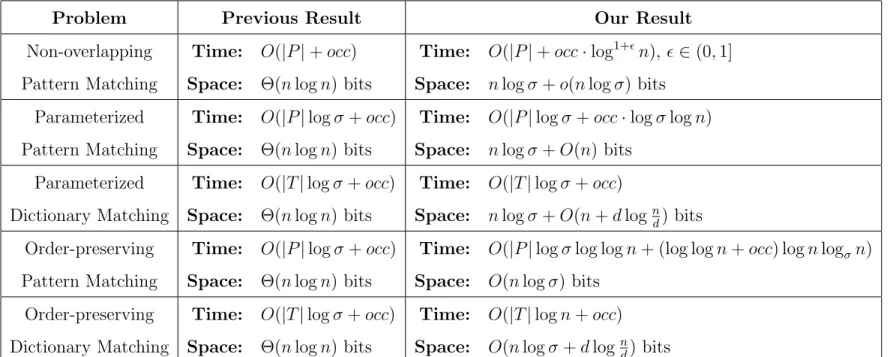
Table 1.1: Our Contribution

Problem Previous Result Our Result

Non-overlapping Pattern Matching Time: Space: O(|P|+occ) Θ(nlogn) bits Time: Space: O(|P|+occ·log1+_n_),_∈₍₀_,_1]

nlogσ+o(nlogσ) bits Parameterized Pattern Matching Time: Space: O(|P|logσ+occ) Θ(nlogn) bits Time: Space:

O(|P|logσ+occ·logσlogn)

nlogσ+O(n) bits Parameterized Dictionary Matching Time: Space: O(|T|logσ+occ) Θ(nlogn) bits Time: Space: O(|T|logσ+occ) nlogσ+O(n+dlog n d) bits Order-preserving Pattern Matching Time: Space: O(|P|logσ+occ) Θ(nlogn) bits Time: Space:

O(|P|logσlog logn+ (log logn+occ) lognlogσn)

O(nlogσ) bits Order-preserving Dictionary Matching Time: Space: O(|T|logσ+occ) Θ(nlogn) bits Time: Space: O(|T|logn+occ) O(nlogσ+dlog n d) bits

(19)

Chapter 2 Preliminaries

We refer the reader to [Gus97] for standard definitions and terminologies. We employ the standard Word-RAM model of computation with poly-logarithmic word size and unit cost for simple CPU operations and memory access. Let T be a string (called text) having n

characters and P be a string (called pattern) having |P| characters. The characters in T

and P are chosen from a totally ordered alphabet Σ having σ characters. Thus, the space occupied by the text is ndlogσe bits. We assume, without loss of generality, that σ ≤ n. Also, assume thatT terminates in a unique special character $. LetT[i, j] be the substring ofT fromitoj (both inclusive) andT[i] be theith character ofT. Further,Tiis the circular

suffix that starts at i. Specifically, Ti = T if i = 1; otherwise, Ti = T[i, n]◦T[1, i−1],

where ◦ denotes concatenation. Lastly, is an arbitrarily small positive constant.

The pattern matching problem asks to answer the following query: report the starting positions (occurrences) i of all substrings of T such that T[i+k−1] =P[k], 1≤k ≤ |P|. In the indexing problem, the textT is fixed, and the objective is to pre-process it and then create a data structure, such that we can answer the above query without having to readT

entirely. We now present some useful definitions and discuss some key data structures that are pivotal in (compressed) text indexing. For dictionary matching, we leave the burden of definitions to the respective chapters.

2.1 Linear vs Compact vs Succinct

An index ofT is a data structure that allows efficient pattern matching queries onT. Here, efficient means that the time to report all occoccurrences isO((|P|+occ) polylog(n)). An index is linear if it occupies Θ(nlogn) bits (or equivalently, Θ(n) words), compact if it occupies Θ(nlogσ) bits, and succinct if it occupiesnlogσ+o(nlogσ) +O(n) bits1_.

1 _{We deviate, albeit very slightly, from the original definition of a succinct index in which the space is}

nlogσ+o(nlogσ) bits. If we wish to stick to the standard definition, for parameterized pattern matching, assumeσ=ω(1). Consequently, the aberration does not violate the original definition asn=o(nlogσ). In the case of a constantσ, we first create all possible copies ofP, where each copy is obtained by replacing

(20)

2.2 Suffix Tree and Suffix Array

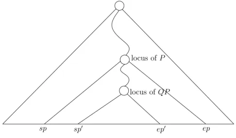
A suffix tree, denoted byST, is a compact trie that stores all the (non-empty) suffixes ofT. Leaves in the suffix tree are numbered in the lexicographic order of the suffix they represent, and each edge in STis labeled by a substring of T. For any node u in the suffix tree, the first character on each edge from uto its child (if any) is unique. Letpath(u) be the string formed by concatenating the edge labels from the root to u; let strDepth(u) = |path(u)|. The locus of a patternP, denoted bylocus(P), is the highest nodeusuch thatP is a prefix of path(u). The suffix range of P is denoted by [sp, ep], where sp(resp. ep) is the leftmost (resp. rightmost) leaf in the subtree of STrooted at the locus of P. (See Figure 2.1 for an illustration.) Usually, each node is equipped with perfect hashing [FKS84] such that given a character x, we can find the outgoing edge whose label begins withxinO(1) time. Then, the locus node (or equivalently, the suffix range) of a patternP is computed in timeO(|P|). Without hashing, the suffix range can be computed in timeO(|P|logσ) via a binary search on the first character of the outgoing edges (recall that leaves are arranged in lexicographic order of the suffixes; hence edges are also arranged in lexicographic order).

The suffix array, denoted bySA, is an array of lengthnthat maintains the lexicographic arrangement of all the suffixes of T. More specifically, if theith smallest suffix of T starts atj, thenSA[i] =j and SA−1[j] =i. The former is referred to as thesuffix array value and the latter as the inverse suffix array value. (See Table 2.1 for an illustration.) The suffix value SA[·] and the inverse suffix value SA−1_[_·_{] can be found in constant time.}

Thus, given the suffix tree and suffix array combination, we can find alloccoccurrences of a pattern P inO(|P|+occ) time – first find the suffix range [sp, ep] ofP using the suffix tree, and then decode SA[i] for everyi∈[sp, ep] to report the occurrences. The suffix tree

the symbols inP with a subset of the symbols in Σ in a one-to-one fashion. Now, for each copy issue an exact pattern matching query on any traditional compressed index [NM07], and get the answers. Since the copies are basically all possible parameterized matches ofP to strings over Σ, we will get the desired occurrences. Note that the number of copies is at most σ!. Hence, the query time is affected by a σ! multiplicative factor, which is still a constant, resulting in succinct indexes with slightly different time complexities (as compared to our results for these problems). Hence, we stick to the modified definition and exclude ourselves from dealing with this rather “boring” case. For order-isomorphic matching, we present a compact index; therefore, the succinct definition is irrelevant.

(21)

$

a

na

1 na

$

na

$

na

$

banana

$

2

3

4

5

6

7 v

Figure 2.1: Suffix Tree for text banana$. We assume $ ≺ a ≺ b ≺ n, where ≺ denotes the total lexicographic order on the alphabet set {$, a, b, n}. Here, locus(an) = v and

path(v) =ana. Suffix range of an is [3,4].

contains nleaves (one per each suffix) and at most (n−1) internal nodes. The suffix array is a permutation on n. Therefore, the space required by these data structures is Θ(nlogn) bits, or equivalently Θ(n) words.

2.3 Burrows-Wheeler Transform and FM-Index

Compressed Suffix Arrays/FM Index reduce the space occupancy of suffix trees/arrays from

Θ(nlogn) bits to O(nlogσ) bits (or close to the size of the text) with a slowdown in query time. Using these data structures, for any pattern P, we can find all occ occurrences in time O((|P|+occ) logcn) for some constant c > 0. We present a brief outline of the FM Index (see [FM05] for more details).

Burrows and Wheeler [BW94] introduced a reversible transformation of the text, known as the Burrows-Wheeler Transform (BWT). Recall that Tx is the circular suffix starting at

position x. Then, BWT of T is obtained as follows: first create a conceptual matrix M, such that each row ofM corresponds to a unique circular suffix, and then lexicographically sort all rows. Thus the ith row in M is given by TSA[i]. The BWT of the text T is the

last column L of M, i.e., BWT[i] =TSA[i][n]. (See Table 2.1 for an illustration.) Note that

(22)

Table 2.1: Here the text isT[1,7] = banana$, where Σ ={a, b, n}. The total lexicographic order on Σ is $≺a ≺b≺n. i Ti TSA[i] (Matrix M) SA[i] SA−1[i] BWT[i] =T[SA[i]−1] LF(i) 1 banana$ $banana 7 5 a 2 2 anana$b a$banan 6 4 n 6 3 nana$ba ana$ban 4 7 n 7 4 ana$ban anana$b 2 3 b 5 5 na$bana banana$ 1 6 $ 1 6 a$banan na$bana 5 2 a 3 7 $banana nana$ba 3 1 a 4

2.3.1 Last-to-First Column Mapping

The underlying principle that enables pattern matching using an FM-Index [FM00] is the last-to-first column mapping (in short, LF mapping). For any i ∈ [1, n], LF(i) is the row

j in the matrix M where BWT[i] appears as the first character in TSA[j]. Specifically,

LF(i) =SA−1_[_SA_[_i_]₋_{1], where} _SA_{[0] =} _SA_[_n_{]. Once the BWT is obtained,} _LF₍_i_{) for any}

suffix i is computed as:

LF(i) = count(1, n,1,BWT[i]−1) +count(1, i,BWT[i],BWT[i])

Here,count(i, j, x, y) counts the number of positionsk∈[i, j] that satisfyx≤BWT[k]≤ y. By maintaining a Wavelet-Tree [GGV03] overBWT[1, n] innlogσ+o(n) bits,count(i, j, x, y) is computed inO(logσ) time (see Fact 2.3 for more details). Hence, we can implement LF mapping in the same space-and-time bounds.

2.3.2 Simulating Suffix Array via LF Mapping

We can decode SA[i] in O(log1+_n_{) time by using LF mapping and by maintaining a}

sampled-suffix array, which occupies o(nlogσ) bits in total. The idea is to explicitly store

SA[i] iff SA[i] ∈ {1,1 + ∆,1 + 2∆, . . .}, where ∆ = dlogσnlog

ne. The space needed is

O(n

(23)

Algorithm 1 Backward Search 1: procedure backwardSearch(P[1, p]) 2: c←P[p], i←p 3: sp ←1 +count(1, n,1, c−1), ep←count(1, n,1, c) 4: while (sp≤ep and i≥2) do 5: c←P[i−1] 6: sp←1 +count(1, n,1, c−1) +count(1, sp−1, c, c)

7: ep←count(1, n,1, c−1) +count(1, ep, c, c)

8: end while

9: if (sp < ep) then “no match found” else return[sp, ep]

10: end procedure

explicitly stored; otherwise, it can be computed via at most ∆ number of LF mapping operations in time O(∆·logσ) =O(log1+n).

2.3.3 Backward Search

Ferragina and Manzini [FM00] showed that using LF mapping, the suffix range [sp, ep] of a pattern P[1, p] can be found by reading P starting from the last character. Specifically, for i >1, suppose the suffix range of P[i, p] is known. Then, the suffix range of P[i−1, p] can be obtained using LF mapping; see Algorithm 1 for details.

Once the suffix range [sp, ep] ofP is known, eachi∈[sp, ep] corresponds to an occurrence of P in T. Each occurrence can be reported in time O(log1+n) as discussed before. Therefore, we arrive at the following well-known result.

Fact 2.1 ([FM05, GV05]). By using an nlogσ+o(nlogσ)-bit index of T, we can find all occurrences of P in T in O(|P|logσ+occ·log1+_n₎ _time.

2.4 Rank and Select on Bit-Vectors

Fact 2.2([Mun96]). LetB[1, m]be a bit-vector. By maintaining ano(m)-bit data structure,

we can find the answer to the following queries in O(1) time:

(a) rankB(i, x) = the number of occurrences of x in B[1, i].

(b) selectB(k, x) = the minimum position i∈[1, m] such that rankB(i, x) =k.

(24)

(d) selectB(i, k, x) = the minimum position j in [i, m] such that rankB(i, j, x) =k.

We drop the subscript B when the context is clear.

2.5 Wavelet Tree

Fact 2.3 ([FM05, GGG+_{07, GGV03, Nav14])}_. _{The wavelet tree (WT) data structure}

gen-eralizes the rank and select queries over bit-vectors. Specifically, given an array A[1, m]

over an alphabet Σ of size σ, by using a data structure of size mlogσ +o(m) bits, the

following queries can be answered in O(1 + _{log log}logσ_m) time: (a) A[i].

(b) rankA(i, x) = the number of occurrences of x in A[1, i].

(c) selectA(k, x) = the minimum position i such that rankA(i, x) = k.

(d) countA(i, j, x, y) = the number of positions k ∈[i, j] such that x≤A[k]≤y.

Additionally, the following queries can be answered in O(logσ) time:

(a) predecessor_A(i, W) = rightmost position j < i such that A[j]≤W.

(b) prevVal_A(L, R) = rightmost position j ∈ [L, R) such that A[j] equals the maximum value in A[L, R−1] that is at most A[R].

(c) nextValA(L, R) = rightmost position j ∈ [L, R) such that A[j] equals the minimum

value in A[L, R−1] that is at least A[R].

We drop the subscript A when the context is clear.

2.6 Succinct Trees with Full Functionality

Fact 2.4 ([NS14]). A tree having m nodes can be represented in 2m+o(m) bits, such that

if each node is labeled by its pre-order rank, we can compute the following in O(1) time:

(a) pre-order(u)/post-order(u) = pre-order/post-order rank of node u. (b) parent(u) = the parent of node u.

(25)

(d) child(u, q) = the qth leftmost child of node u.

(e) sibRank(u) = number of children of parent(u) to the left of u.

(f ) lca(u, v) = the lowest common ancestor (LCA) of two nodes u and v.

(g) lmostLeaf(u)/rmostLeaf(u) = the leftmost/rightmost leaf in the subtree rooted at u. (h) levelAncestor(u, D) = the ancestor of u such that nodeDepth(u) =D.

(i) the pre-order rank of the ith leftmost leaf

(j) leafNumber(`) = the number of leaves that lie to the left of the leaf `.

2.7 Succinctly Indexable Dictionaries

Fact 2.5 ([RRS07]). A set S of k integer keys from a universe of size U can be stored in

klog(U/k) +O(k) bits of space to support the following two operations in O(1) time:

(a) return the key of rank i in the natural order of integers.

(26)

Chapter 3 Succinct Index for Non-overlapping

Pattern Matching

We begin by formally defining the Non-overlapping Indexing problem.

Problem 3.1(Non-overlapping Indexing). Two occurrences of a pattern P in a textT[1, n]

are non-overlapping iff they are separated by at least |P|positions, i.e., for two occurrences

t and t0_, _|_t₋_t0_{| ≥ |}_P_|_{. The task is to index} _T _{such that we can efficiently report a set}

containing the maximum number of non-overlapping occurrences of P in T.

For example, if T = ababaxyaba and P = aba, then we have to report the position 8 and either 1 or 3 (but not both). We observe that there can be multiple sets of maximum non-overlapping occurrences. Our objective is to report any one set.

Cohen and Porat [CP09] presented the first optimal time solution to this problem. Their index, consisting of a suffix tree of T and an additional O(n)-word data structure, can report all thenoccnon-overlapping occurrences in timeO(|P|+nocc). However, it was left unanswered, whether Problem 3.1 can be handled in succinct (or, compact) space, or not. We answer this affirmatively by showing that the problem can be solved efficiently using any index of T alone, as summarized in the following theorem.

Theorem 3.1. Let CSAbe a full-text index ofT. UsingCSA, let (i)search(P) = Ω(|P|) be

the time in which we can compute the suffix range of P, and (ii) tSA= Ω(1) be the time in

which we can compute a suffix array or inverse suffix array value. By using CSA alone, we

can find a set containing the maximum number, say nocc, of non-overlapping occurrences

of P in time O(search(P) +nocc·(tSA+ lognocc)).

Thus, Problem 3.1 can be solved using any text-index (succinct, compact, or linear space) for the traditional problem of reporting all occurrences. Furthermore, by avoiding the use of any additional data structures, we ensure that various space and time trade-offs

(27)

can be easily obtained. For example, if we use a suffix tree, O(|P|+nocclognocc) time can be obtained. This is very similar to the result by Cohen and Porat [CP09], and in fact, by using some additional O(nlogn)-bit data structures (used by Cohen and Porat as well), the query time can be improved to optimal O(|P|+nocc). On the other hand, an

nlogσ+o(nlogσ)-bit andO(|P|+nocc·log1+_n_{) time index can be obtained by using the}

compressed suffix array of Belazzougui and Navarro [BN14]; note that nocc ≤ n. Recall that σ is the size of the alphabet and >0 is an arbitrary small constant.

3.1 Overview of Techniques

The non-overlapping occurrences can be found as follows: find alloccoccurrences in sorted order, report the last occurrence, then perform a right to left scan of the occurrences, and report an occurrence if it is at least|P|characters away from the latest reported occurrence. Consider the text in Figure 3.1. The occurrences (in sorted order) of the pattern

P =abaare the positions 4,9,11,13,21,23. Following the procedure above, we first report 23. Then, skip 21, report 13, skip 11, and report 9. Finally, we report 4 and terminate.

The complexity of this procedure isO(search(P) +occ·tSA+occ·logocc); the first two

factors are for finding all the occurrences and the third one is for sorting the occurrences. The idea behind reducing the complexity to that claimed in Theorem 3.1 is to consider at most nocc occurrences (instead of occoccurrences) initially.

We break down the occoccurrences into maximal disjoint chains of occurrences – each successive occurrence in a chain are regularly separated, say by x <|P| positions, but the first and last occurrence of two successive chains are separated by at least|P|positions. We repeat the following steps for each chain. Start from the rightmost occurrence in a chain, and report it. Use x and |P| to find the closest occurrence which is at least|P|characters to the left of the latest reported one. Now, we report this previous occurrence and repeat until the entire chain is consumed.

It is not too hard to see that if we consider O(nocc) chains initially and spend O(tSA)

(28)

our strategy – find the chains and then query each chain; Section 3.3 contains the details. We begin with a few basic ingredients in Section 3.2.

3.2 Definitions

In what follows, we use CSAto denote a full-text index of T (not necessarily a compressed index). Using CSA, letsearch(P) = Ω(|P|) be the time in which we can compute the suffix range of P, and tSA= Ω(1) be the time in which we can compute a suffix array or inverse

suffix array value. We assume that search(P) is proportional to|P|.

Lemma 3.1. Given the suffix range [sp, ep]of patternP, using CSA, we can verify in time O(tSA) whether P occurs at a text-position t, or not.

Proof. The lexicographic position`of the suffixT[t, n] (i.e.,SA−1[t]) can be found inO(tSA)

time. The lemma follows by observing that P occurs at t iff sp≤`≤ep.

Definition 3.1 (Period of a Pattern). The period of a pattern P is its shortest non-empty

prefix Q, such thatP can be written as the concatenation of several (say α >0) number of

copies of Q and a (possibly empty) prefix Q0 of Q. Specifically, P =Qα_Q0_.

The period of P can be computed O(|P|) time using the failure function of the KMP

algorithm [Gus97, KJP77].

For example, if P = abcabcab, then Q = abc, α = 2, and Q0 ₌ _ab_{. If} _P ₌ _aaa_{, then}

Q=a, α= 3, and Q0 _{is empty. If} _P ₌_abc_{, then} _Q₌_abc_,_α _{= 1, and} _Q0 _{is empty.} The following is an important observation related to periodicity of strings.

Observation 3.1. Two occurrences of a pattern P = Qα_Q0 _{are separated by at least} _|_Q_| characters, i.e., if t is an occurrence, then the closest occurrence can be at t± |Q|.

3.3 The Querying Process

In this section, we present our solution to Problem 3.1. Moving forward, assume that P

has been decomposed as Qα_Q0_{, which can be computed in} _O₍_|_P_|_{) time using the failure} function of the KMP algorithm [Gus97, KJP77]. We also assume that the suffix range of

(29)

3.3.1 Aperiodic Patterns

If P does not occur in T, Problem 3.1 can be trivially answered using CSA in search(P) time. Also, observe that P can overlap itself iff there is a proper suffix of P which is also its (proper) prefix; in this case, Q is a proper prefix of P = Qα_Q0_{. If this condition} does not hold (i.e., if Q = P), which can be verified in O(|P|) time using the KMP algorithm [Gus97, KJP77], then the desired non-overlapping occurrences are simply all the occurrences of P (i.e., nocc=occ), which can be found in time O(search(P) +nocc·tSA).

Now, we consider the case when α = 1 (i.e., P =QQ0_{) and} _Q0 _{is not empty. In other} words, P has a proper prefix which is also its proper suffix. In this case, note that occ≤ 2nocc. Therefore, we can simply find all occurrences using CSAinO(search(P) +occ·tSA)

time. Then sort the occurrences and use the naive algorithm at the beginning of Section 3.1 to find the a set containing the desired nocc number of non-overlapping occurrences in

O(search(P) +nocc·(tSA+ lognocc)) time. Summarizing, we get the following lemma

Lemma 3.2. Given a patternP, we can check if it has any occurrence inT inO(search(P))

time. If there is no proper suffix of P which is also its proper prefix, then we can find all

the non-overlapping occurrences in O(search(P) +nocc·tSA)time. Lastly, if P =QQ0 and

Q0 is not empty, then we can find all the non-overlapping occurrences in O(search(P) +

nocc·(tSA+ lognocc)) time.

3.3.2 Periodic Patterns

In this case, P =Qα_Q0_{, where}_α _≥_{2. We begin with the following definitions.}

Definition 3.2 (Critical Occurrence). A position tc in T is called a critical occurrence of

P =Qα_Q0_{, where} _α_≥₂_{, iff} _t

c is an occurrence of P but the position tc+|Q| is not.

Definition 3.3 (Range of a Critical Occurrence). Let tc be a critical occurrence of P in

T. Let t0 _≤_t

c be the maximal position such thatt0, t0+|Q|, t0+ 2|Q|, . . . , tc are occurrences

of P but the position t0_{− |}_Q_| _{is not. The range of} _t

(30)

For example, let the text T[1,18] be xyzabcabcabcabxyx$. Then tc = 7 is a critical

occurrence of P =abcabcab, but tc = 4 is not. Also,range(7) = [4,14].

Following are some crucial observations.

Observation 3.2. Let tcbe a critical occurrence ofP. Then, tcis the rightmost occurrence

of P in range(tc). Furthermore, the ranges of two critical occurrences are disjoint.

Observation 3.3. A critical occurrence ofP inT corresponds to at least one non-overlapping

occurrence, i.e., nocc is at least the number of critical occurrences of P in T.

It follows from Observations 3.2 and 3.3 that to find the desired non-overlapping occur-rences of P in T, it suffices to find the maximum number of non-overlapping occurrences of P in the range of every critical occurrence. Clearly the following two components suffice – (i) an algorithm that finds the maximum number of non-overlapping occurrences of P

in the range of a single critical occurrence, and (ii) an algorithm that can find all critical occurrences ofP. The first component is met by Lemma 3.3 and the second by Lemma 3.4.

Lemma 3.3. Given a pattern P =Qα_Q0 _{in the form}_h|_Q_|_{, α,}_|_Q0_|i _{for some} _α_≥₂_{, and the}

suffix range ofP, we can find a set of the maximum number of non-overlapping occurrences

of P in range(tc) in timeO(nocc0·tSA), wherenocc0 is the size of the set and tc is a critical

occurrence of P.

Proof. The proof is immediate from the following steps. See Figure 3.1 for an illustration.

1. Reporttc as a non-overlapping occurrence of P.

2. Let t=tc−α|Q|. If t≤0 or if P does not appear att (which can be verified intSA

time using Lemma 3.1), then terminate. Otherwise, t belongs to range(tc). If Q0 is

empty, then let t0 =t− |Q|, else t0 =t.

3. If t0 _≤ _{0 or if} _P _{does not appear at} _t0_{, then terminate. Otherwise} _t0 _{belongs to}

range(tc), and is the closest occurrence (in range(tc)) to tc such that t0 and tc are at

(31)

Figure 3.1: Illustration of Lemma 3.3. Top row shows the text, and bottom row shows the corresponding text position. Shaded text positions mark the critical occurrences of the pattern P =aba for which Q=aband Q0 ₌_a_{. Shaded text region shows the range of the} critical occurrences tc;t and t0 have the same meaning as in Lemma 3.3.

4. By lettingtc=t0, repeat the process starting from Step 2.

Clearly, at the end of the process described above, the desired nocc0 _{occurrences of} _P _in

range(tc) are reported in O(nocc0·tSA) time.

Our next task is to find all critical occurrences of P in T. The following lemma shows how to achieve this.

Lemma 3.4. Given a pattern P =Qα_Q0_{, we can find all critical occurrences of} _P _in _T _in time bounded by O(search(P) +nocc·tSA).

Proof. The proof relies on the following observation: a critical occurrence of a pattern P

is the same as the text position of a leaf which belongs to the suffix range of P, but not of

QP. If this is not true, then there is a critical occurrence ofP, say at positiontc, such that

SA−1[tc] lies in the suffix range of QP =Qα+1Q0. But then there is an occurrence of P at

the position t =tc+|Q|, a contradiction.

Since Q0 is a prefix of Q, note that the suffix range of QP is contained within that of

P; see Figure 3.2. Therefore, our objective translates to locating the suffix range ofP, say [sp, ep], and of QP, say [sp0_{, ep}0_{]. This can be achieved in time} _search₍_QP_{), which can be} bounded by O(search(P)). (Recall that search(P) is proportional to |P|.)

For each leaf ` lying in [sp, sp0₋_1]_∪_[_ep0_{+ 1}_{, ep}_{], the text position} _SA_[_`_{] is a (distinct)} critical occurrence of P. Thus, the total number of these leaves is same as the number of critical occurrences of P in T. By Observation 3.3, the number of critical occurrences is at most the output size nocc. For every leaf `, we can find the corresponding critical

(32)

locus ofP

locus ofQP

sp sp0 _ep0 _ep

Figure 3.2: Illustration of Lemma 3.4. Since, Q0 _{is a prefix of} _Q_{, the locus of} _P ₌ _Qα_Q0 lies on the path from root to the locus of QP. For each leaf ` in [sp, sp0−1]∪[ep0+ 1, ep], the text position SA[`] is a critical occurrence ofP.

occurrence (i.e., its text position) in time tSA usingSA[`]. Therefore, once the suffix ranges

of P and QP are located, all the critical occurrences are found in timeO(nocc·tSA).

From Lemma 3.3, we conclude that given the suffix range of P (which can be found in

search(P) time) and every critical occurrence of P inT, we can find the desired nocc non-overlapping occurrences of P in time O(search(P) +nocc·tSA). Every critical occurrence

of P can be found using Lemma 3.4 in O(search(P) +nocc·tSA) time. By combining these

(33)

Chapter 4 Succinct Index for Parameterized

Pattern Matching

We begin with the definition of the parameterized matching. Here, the alphabet Σ is the union of two disjoint sets: Σs, the set ofσs static characters (s-characters), and Σp, the set

of σp parameterized characters (p-characters). Thus, σ=|Σ|=σs+σp.

Definition 4.1 (Parameterized Matching [Bak93]). Two equal-length stringsS andS0 over

Σ are a parameterized match (p-match) iff

• S[i]∈Σs ⇐⇒ S0[i]∈Σs,

• S[i] =S0_[_i_] _when _S_[_i_]_∈_Σ s, and

• there exists a one-to-one matching-function f that renames the p-characters in S to

the p-characters in S0_{, i.e.,} _S0_[_i_{] =}_f₍_S_[_i_]) _when _S_[_i_]_∈_Σ p.

For example, let Σs = {A, B, C,$} and Σp = {w, x, y, z}. Then, S = AxByCx

p-matches S0 =AzBwCz, where the matching function f is: f(x) =z and f(y) =w. Also,

S p-matches S0 ₌ _AyBxCy _with _f₍_x_{) =} _y _and _f₍_y_{) =} _x_{. However,} _S _{is not a p-match} with S0 ₌_AwBxCz _as _x_in _S _{would have to match with both}_w _and _z _in _S0_.

The Parameterized Text Indexing problem is a generalization of the standard

text-indexing problem, with the match between two strings replaced by a p-match. Specifically,

Problem 4.1 (Parameterized Text Indexing [Bak93]). Let T be a text of length n over Σ = Σs∪Σp. We assume that T terminates in an s-character $ which appears only once.

Index T, such that for a pattern P (also over Σ), we can report all the p-occurrences of P,

i.e., all the starting positions of the substrings of T that are a p-match with P.

For the above problem, Baker [Bak93] presented a linear-space index, known as the

(34)

find all the p-occurrences of P in O(|P|logσ+occ) time, where occ is the number of p-occurrences of P. We present the following new result, which occupies (much) lesser space for a slightly higher query time.

Theorem 4.1. By using an nlogσ+O(n)-bit index of T, the p-occurrences of P can be found in O(|P|logσ+occ·lognlogσ)time, where occis the number of such p-occurrences. If we are allowed slightly higher space, then we can obtain the following result as an immediate consequence of our techniques for proving Theorem 4.1 above.

Theorem 4.2. By using an O(nlogσ)-bit index ofT, the p-occurrences of P can be found

in O(|P|logσ+occ·logn) time, where occ is the number of such p-occurrences.

4.1 Overview of Techniques

The key idea to obtain the linear-space index of Baker [Bak93] for Problem 4.1 is an encoding scheme, such that two strings are a p-match iff their encoded strings are a match in the traditional sense. The encoding scheme was introduced by Baker [Bak93], which led to the parameterized suffix tree (p-suffix tree) – encode each suffix of T and then create a compact trie of these encoded suffixes. Reporting the occurrences of a pattern is now trivial using the encoded P, the p-suffix tree, and the techniques introduced in Section 2.2. We first find the highest node u in the p-suffix tree such that the string obtained by concatenating the edge labels from root to u is prefixed by the encoded pattern. Then, we report the starting positions of the encoded suffixes corresponding to the leaves in the subtree of u. Although this uses lesser time than Theorem 4.1, the space required by the p-suffix tree is much higher than the text itself. We present the details in Section 4.2.

At this point, one may be tempted to think that we can apply the techniques of the FM-Index [FM05] to get a succinct equivalent of the p-suffix tree; see Section 2.3. The FM-Index (as does the Compressed Suffix Array [GV05]) relies on a crucial property of suffixes: any two suffixes which have the same preceding character c (in text order) will retain their relative lexicographic rank when they are prepended by c. Unfortunately, in

(35)

case of Baker’s encoded suffixes, this property no longer holds. Consequently, FM-Index and CSA no longer work. The reason why encoded suffixes do not follow this property is that on prepending the preceding character, the encoding of the original suffix changes. Fortunately, this change happens at exactly one position. The key idea is to identify this position of change. However, we cannot explicitly store this position of change as it needs ≈ logn bits per suffix. Instead, we store the number of distinct p-characters upto this position (from the start of the suffix). This information, which can be stored in ≈ logσ

bits per suffix, forms the backbone of our index. We call it the Parameterized

Burrows-Wheeler Transform (pBWT); the details are in Section 4.3.

The main ingredient after obtaining pBWT is to implement an analogous version of the LF mapping of the FM-Index (see Section 2.3.1), which we call the Parameterized LF

mapping (pLF mapping); see Section 4.4 for details. Recall that using LF mapping, we can

simulate the suffix array without explicitly storing it; see Section 2.3.2. Similarly, using pLF mapping, we can simulate the parameterized suffix array, which stores the starting positions of the lexicographically arranged encoded suffixes; the techniques are standard and Theorem 4.3 presents a formal description.

Summarizing our discussions this far, we can see that the key is to compute pLF mapping. To this end, we use the pBWT and the topology of the p-suffix tree; the crucial insight is provided in Lemma 4.1. Based on this lemma, we implement pLF mapping in Section 4.5; space and time complexities are described in Theorem 4.4.

The last piece of the puzzle is to compute the suffix range of the encoded pattern (i.e., find the range of leaves under the node u defined at the beginning of this section). We again use pLF mapping, the tree topology, and pBWT to implement an analogous version of the backward search procedure of the FM Index (see Section 2.3.3). The details of the backward search procedure for p-matching is in Section 4.6.

(36)

4.2 Parameterized Suffix Tree

We now present the following encoding scheme introduced by Baker [Bak93].

Definition 4.2 (Baker’s Encoding). We encode any string S overΣ into a string prev(S) of length |S| as follows: prev(S)[i] =                S[i] if S[i] is an s-character,

0 else if i is the first occurrence of S[i] in S,

i−j otherwise, where j is the last occurrence of S[i] before i in S.

In other words,prev(S) is obtained by replacing the first occurrence of every p-character in S by 0 and any other occurrence by the difference in text position from its previous occurrence. For example,prev(AxByCx) =A0B0C4, whereA, B ∈Σs and x, y ∈Σp. The

time required to compute prev(S) is O(|S|logσ)1_.

Fact 4.1 ([Bak93]). Two strings S and S0 are a p-match iff prev(S) =prev(S0). AlsoS is a p-match with a prefix of S0 iff prev(S) is a prefix of prev(S0).

Note that prev(S) is a string over an alphabet set Σs ∪ {0,1, . . . ,|S| −1}. Moving

forward, we follow the convention below.

Convention 4.1. The integer characters (corresponding to p-characters) are

lexicograph-ically smaller than s-characters. An integer character i comes before another integer

char-acter j iff i < j. Also, $ is lexicographically larger than all other characters.

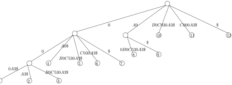
Parameterized Suffix Tree (pST) is the compacted trie of all strings in {prev(T[k, n])| 1≤k ≤n}. Clearly, pSTconsists ofn leaves and at most n−1 internal nodes. Each edge is labeled with a sequence of characters from Σ0 _{= Σ}

s∪ {0,1, . . . , n−1}. See Figure 4.1 for

an illustration. We use path(u) to denote the concatenation of edge labels on the path from

1 _{Maintain a balanced binary search tree} _T_{, which is initially empty. Scan} _S _{from left to right, and}

supposex∈Σpappears in positionk. Ifx /∈ T, then assignprev(S)[k] = 0, and insertxintoT. Otherwise,

(37)

root to node u, andstrDepth(u) =|path(u)|. The path of each leaf node corresponds to the encoding (using Definition 4.2) of a unique suffix of T, and leaves are ordered according to the lexicographic rank of the corresponding encoded suffixes. We use `i to denote the leaf

corresponding to theith lexicographically smallestprev-encoded suffix, i.e., theith leftmost leaf inpST. Thus,path(`i) = prev(T[pSA[i], n]), wherepSA[1, n] is theParameterized Suffix

Array, which maintains the lexicographic arrangement of all the encoded suffixes of T. In

particular, pSA[i] =j and pSA−1_[_j_{] =}_i_iff _prev₍_T_[_{j, n}_{]) is the}_i_{th lexicographically smallest}

string in {prev(T[k, n])|1≤k ≤n}.

UsingpST, searching for all occurrences ofP inT is straight-forward as follows. Simply traverse pST from root by following the edges labels and find the highest node u (called locus) with its path prefixed by prev(P). Then find the range [sp, ep] (called suffix range) of leaves in the sub-tree of u and report {pSA[i]|sp≤i≤ep} as the output.

The space occupied by pST is Θ(n) words (or equivalently, Θ(nlogn) bits), and the query time is O(|P|logσ+occ), assuming perfect hashing [FKS84] at each node.

4.3 Parameterized Burrows-Wheeler Transform

We introduce a reversible transformation similar to that of the Burrows-Wheeler Trans-form [BW94]. We call this the Parameterized Burrows-Wheeler TransTrans-form (p-BWT). To obtain the p-BWT ofT, we first create a conceptual matrixM, where each row corresponds to a unique circular suffix of T. Then, we sort all the rows lexicographically according to the prev(·) encoding of the corresponding unique circular suffix and obtain the last column

L of the sorted matrix M. Clearly, the ith row is equal to TpSA[i]. Moving forward, denote

by fi, the first occurrence of L[i] =TpSA[i][n] in TpSA[i]. (Note that fi is defined.)

The p-BWT of T, denoted by pBWT[1, n], is defined as follows:

pBWT[i] =        L[i], if L[i] is an s-character,

(38)

0 A0 B0C030A3$ C000A3$ 11 $ 12 10 $ 0B0C530A3$ A0$ 8 9 B0C530A3$ C030A3$ $ 4 5 6 7 0 0A3$ A3$ B0C530A3$ 1 2 3

Figure 4.1: Parameterized Suffix Tree for text AxyBzCxzwAz$, where Σs = {A, B, C,$} and Σp = {w, x, y, z}. We assume

(39)

Table 4.1: Here the text is T[1,12] =AxyBzCxzwAz$, where Σs ={A, B, C,$} and Σp ={w, x, y, z}

i Ti prev(Ti) prev(TpSA[i]) TpSA[i] pSA[i] L[i] fi pBWT[i] pLF(i)

1 AxyBzCxzwAz$ A00B0C530A3$ 000A3$A70B6C xzwAz$AxyBzC 7 C C 11

2 xyBzCxzwAz$A 00B0C530A3$A 00A3$A00B6C5 zwAz$AxyBzCx 8 x 7 3 1

3 yBzCxzwAz$Ax 0B0C030A3$A7 00B0C530A3$A xyBzCxzwAz$A 2 A A 8

4 BzCxzwAz$Axy B0C030A3$A70 0A0$A00B6C53 wAz$AxyBzCxz 9 z 3 2 2

5 zCxzwAz$AxyB 0C030A3$A70B 0B0C030A3$A7 yBzCxzwAz$Ax 3 x 5 3 3

6 CxzwAz$AxyBz C000A3$A70B6 0C030A3$A70B zCxzwAz$AxyB 5 B B 10

7 xzwAz$AxyBzC 000A3$A70B6C 0$A00B5C530A z$AxyBzCxzwA 11 A A 9

8 zwAz$AxyBzCx 00A3$A00B6C5 A00B0C530A3$ AxyBzCxzwAz$ 1 $ $ 12

9 wAz$AxyBzCxz 0A0$A00B6C53 A0$A00B5C530 Az$AxyBzCxzw 10 w 12 4 4

10 Az$AxyBzCxzw A0$A00B5C530 B0C030A3$A70 BzCxzwAz$Axy 4 y 12 4 5

11 z$AxyBzCxzwA 0$A00B5C530A C000A3$A70B6 CxzwAz$AxyBz 6 z 3 2 6

(40)

In other words, when L[i] ∈ Σs, pBWT[i] = T[pSA[i]−1] (define T[0] = T[n] = $

and T0 = Tn) and when L[i] ∈ Σp, pBWT[i] is the number of 0’s in the fi-long prefix

of prev(TpSA[i]). Thus, pBWT is a sequence of n characters over the alphabet set Σ00 =

Σs∪ {1,2, . . . , σp} of sizeσs+σp =σ. See Table 4.1 for an illustration of pSA andpBWT.

In order to represent pBWT succinctly, we map each s-character in Σ00 _{to a unique} integer in [σp+ 1, σ]. Specifically, the ith smallest s-character will be denoted by (i+σp).

Moving forward, pBWT[i] ∈ [1, σp] iff L[i] is a p-character and pBWT[i] ∈ [σp + 1, σ] iff

L[i] is a s-character. We summarize the relation betweenprev(TpSA[i]) and prev(TpSA[i]−1) in

Observation 4.1.

Observation 4.1. For any 1≤i≤n,

prev(TpSA[i]−1) =        pBWT[i]◦prev(TpSA[i])[1, n−1], if pBWT[i]> σp,

0◦prev(TpSA[i])[1, fi−1]◦fi◦prev(TpSA[i])[fi+ 1, n−1], otherwise.

4.4 Parameterized LF Mapping

Based on our conceptual matrix M, the parameterized last-to-first column (pLF) mapping of iis the position at which the character at L[i] lies in the first column ofM. Specifically,

pLF(i) =pSA−1[pSA[i]−1], where pSA−1[0] =pSA−1[n]; see Table 4.1. The significance of

pLF mapping is summarized in the following theorem.

Theorem 4.3. Assume pLF(i) for any i∈[1, n] is computed intpLF time. For any

param-eter ∆, by maintaining an additional O((n/∆) logn)-bit data structure, we can compute

pSA[j] for any j ∈[1, n] in O(∆·tpLF) time.

Proof. Define, pLF0(i) = i and pLFk(i) = pLF(pLFk−1(i)) = pSA−1[pSA[i]− k] for any integer k >0. We employ perfect hashing [FKS84] to store the hj,pSA[j]i key-value pairs for all j such thatpSA[j] belongs to {1,1 + ∆,1 + 2∆,1 + 3∆, . . . , n}. Using this, given a

j, one can check if pSA[j] has been stored (and also retrieve the value) in O(1) time. The total space occupied is O((n/∆) logn) bits. To find pSA[i], repeatedly apply the pLF(·)

Succinct Data Structures for Parameterized Pattern Matching and Related Problems

Louisiana State University

LSU Digital Commons

Succinct Data Structures for Parameterized Pattern

Matching and Related Problems

Arnab Ganguly

Acknowledgments

Table of Contents

Abstract

Chapter 1

Introduction

1.1

Motivation

1.2

Contribution

Type 1 Applications

1.2.1

Non-overlapping Pattern Matching

Type 2 Applications

1.2.2

Parameterized Pattern Matching

1.2.3

Parameterized Dictionary Matching

1.2.4

Order-preserving Pattern Matching

1.2.5

Order-preserving Dictionary Matching

1.3

Roadmap

Chapter 2

Preliminaries

2.1

Linear vs Compact vs Succinct

2.2

Suffix Tree and Suffix Array

$

a

na

1

na

$

$

na

$

$

na

$

banana

$

2

3

4

5

6

7

v

2.3

Burrows-Wheeler Transform and FM-Index

2.3.1

Last-to-First Column Mapping

2.3.2

Simulating Suffix Array via LF Mapping

2.3.3

Backward Search

2.4

Rank and Select on Bit-Vectors

2.5

Wavelet Tree

2.6

Succinct Trees with Full Functionality

2.7

Succinctly Indexable Dictionaries

Chapter 3

Succinct Index for Non-overlapping

Pattern Matching

3.1

Overview of Techniques

3.2

Definitions

3.3