Working Paper 11-34
Statistics and Econometrics Series
October 2011
BOOTSTRAP FORECAST OF MULTIVARIATE VAR MODELS WITHOUT
USING
THE BACKWARD REPRESENTATION
Lorenzo Pascual
In this paper, we show how to simplify the construction of bootstrap prediction densities in
multivariate VAR models by avoiding the backward representation. Bootstrap prediction
densities are attractive because they incorporate the parameter uncertainty a
any particular assumption about the error distribution. What is more, the construction of
densities for more than one-step
unknown asymptotically. The main advantage of the new
simple without loosing the good performance of bootstrap procedures. Furthermore, by avoiding
a backward representation, its asymptotic validity can be proved without relying on the
assumption of Gaussian errors as
proposed in this paper can be implemented to obtain prediction densities in models without a
backward representation as, for example, models with MA components or GARCH
disturbances. By comparing the finite sample performance of the proposed procedure with those
of alternatives, we show that nothing is lost when using it. Finally, we implement the procedure
to obtain prediction regions for US quarterly future inflation, unemployment and GDP growth
Keywords:
Non-Gaussian VAR models, Prediction cubes, Prediction density, Prediction
regions, Prediction ellipsoids, Resampling methods.
♦
EDP-Energías de Portugal, S.A., Unidade de Neg
♠
Corresponding author: Dpt. Estadística and Instituto Flores de Lemus, Universidad Carlos III de Madrid, C/ Madrid 126, 28903 Getafe, Spain. Tel: 34 916249851, Fax: 34 916249849, e
♣
Dpt. de Estadística, Universidad Carlos III de Madrid, C [email protected].
Acknowledgements. The last two authors are grateful for financial support from project
Statistics and Econometrics Series
026
Departamento de Estadística
Universidad Carlos III de Madrid
Calle Madrid, 126
28903 Getafe (Spain)
Fax (34) 91 624
BOOTSTRAP FORECAST OF MULTIVARIATE VAR MODELS WITHOUT
THE BACKWARD REPRESENTATION
Lorenzo Pascual
♦, Esther Ruiz
♠and DiegoFresoli
♣Abstract
In this paper, we show how to simplify the construction of bootstrap prediction densities in
multivariate VAR models by avoiding the backward representation. Bootstrap prediction
densities are attractive because they incorporate the parameter uncertainty and do not rely on
any particular assumption about the error distribution. What is more, the construction of
step-ahead is possible even in situations when these densities are
unknown asymptotically. The main advantage of the new procedure is that it is computationally
simple without loosing the good performance of bootstrap procedures. Furthermore, by avoiding
a backward representation, its asymptotic validity can be proved without relying on the
assumption of Gaussian errors as needed by alternative procedures. Finally, the new procedure
proposed in this paper can be implemented to obtain prediction densities in models without a
backward representation as, for example, models with MA components or GARCH
the finite sample performance of the proposed procedure with those
of alternatives, we show that nothing is lost when using it. Finally, we implement the procedure
to obtain prediction regions for US quarterly future inflation, unemployment and GDP growth
Gaussian VAR models, Prediction cubes, Prediction density, Prediction
regions, Prediction ellipsoids, Resampling methods.
Energías de Portugal, S.A., Unidade de Negócio de Gestao da Energía, Director Adjunto.
author: Dpt. Estadística and Instituto Flores de Lemus, Universidad Carlos III de Madrid, C/ Madrid 126, 28903 Getafe, Spain. Tel: 34 916249851, Fax: 34 916249849, e-mail: [email protected]
ersidad Carlos III de Madrid, C/ Madrid 126, 28903 Getafe (Madrid), Spain, e The last two authors are grateful for financial support from project ECO2009
Departamento de Estadística
Universidad Carlos III de Madrid
Calle Madrid, 126
28903 Getafe (Spain)
Fax (34) 91 624
-98-49
BOOTSTRAP FORECAST OF MULTIVARIATE VAR MODELS WITHOUT
In this paper, we show how to simplify the construction of bootstrap prediction densities in
multivariate VAR models by avoiding the backward representation. Bootstrap prediction
nd do not rely on
any particular assumption about the error distribution. What is more, the construction of
ahead is possible even in situations when these densities are
procedure is that it is computationally
simple without loosing the good performance of bootstrap procedures. Furthermore, by avoiding
a backward representation, its asymptotic validity can be proved without relying on the
needed by alternative procedures. Finally, the new procedure
proposed in this paper can be implemented to obtain prediction densities in models without a
backward representation as, for example, models with MA components or GARCH
the finite sample performance of the proposed procedure with those
of alternatives, we show that nothing is lost when using it. Finally, we implement the procedure
to obtain prediction regions for US quarterly future inflation, unemployment and GDP growth.
Gaussian VAR models, Prediction cubes, Prediction density, Prediction
author: Dpt. Estadística and Instituto Flores de Lemus, Universidad Carlos III de Madrid, C/ Madrid econ.uc3m.es.
/ Madrid 126, 28903 Getafe (Madrid), Spain, e-mail: ECO2009-08100 of the Spanish
Bootstrap Forecast of Multivariate VAR Models without
using the backward representation
Lorenzo Pascual
∗Esther Ruiz
†Diego Fresoli
‡§October 2011
Abstract
In this paper, we show how to simplify the construction of bootstrap prediction densities in multivariate VAR models by avoiding the backward representation. Bootstrap prediction densities are attractive because they incorporate the parameter uncertainty and do not rely on any particular assumption about the error distribution. What is more, the construction of densities for more than one-step-ahead is possible even in situations when these densities are unknown asymptotically. The main advantage of the new procedure is that it is computa-tionally simple without loosing the good performance of bootstrap procedures. Furthermore, by avoiding a backward representation, its asymptotic validity can be proved without relying on the assumption of Gaussian errors as needed by alternative procedures. Finally, the new procedure proposed in this paper can be implemented to obtain prediction densities in models without a backward representation as, for example, models with MA components or GARCH disturbances. By comparing the finite sample performance of the proposed procedure with those of alternatives, we show that nothing is lost when using it. Finally, we implement the procedure to obtain prediction regions for US quarterly future inflation, unemployment and GDP growth.
KEYWORDS: Non-Gaussian VAR models, Prediction cubes, Prediction density, Predic-tion regions, PredicPredic-tion ellipsoids, Resampling methods.
∗EDP-Energ´ıas de Portugal, S.A., Unidade de Neg´ocio de Gest˜ao da Energ´ıa, Director Adjunto.
†Corresponding author: Dpt. Estad´ıstica and Instituto Flores de Lemus, Universidad Carlos III de Madrid, C/
Madrid 126, 28903 Getafe, Spain. Tel: 34 916249851, Fax: 34 916249849, e-mail: [email protected].
‡Dpt. de Estad´ıstica, Universidad Carlos III de Madrid, C./ Madrid 126, 28903 Getafe (Madrid), Spain, e-mail
§Acknowledgements. The last two authors are grateful for financial support from project ECO2009-08100
of the Spanish Government. We are also grateful to Gloria Gonz´alez-Rivera for her useful comments. The usual disclaims apply.
1
Introduction
Bootstrap procedures are known to be useful when forecasting time series because they allow the construction of prediction densities without imposing particular assumptions on the error distribution and simultaneously incorporating the parameter uncertainty. Note that when the errors are non-Gaussian the prediction densities are usually unknown when the prediction hori-zon is larger than one-step-ahead. However, the bootstrap can be implemented in these cases to obtain the corresponding prediction densities. They are also attractive because their compu-tational simplicity and wide applicability. However, these advantages are limited by the use of the backward representation that many authors advocate after the seminal paper of Thombs and Schuchany (1990). In particular, Kim (1999) extends the procedure of Thombs and Schuchany (1990) to stationary VAR(p) models. Later, Kim (2001, 2004) considered bias-corrected predic-tion regions by employing a bootstrap-after-bootstrap approach. On the other hand, Grigoletto (2005) proposes two further alternative procedures based on Kim (1999) that take into account not only the uncertainty due to parameter estimation but also the uncertainty attributable to model specification. In any case, the bootstrap procedures conceived by Kim (1999, 2001, 2004) and Grigoletto (2005) use the backward representation to generate the bootstrap samples used to obtain replicates of the estimated parameters. Using the backward representation has three main drawbacks. First, the resulting procedure is computationally complicate and time consuming. Second, given that the backward residuals are not independent it is necessary to use the relation-ship between the backward and forward representation of the model in order to resample from independent residuals; see Kim (1997, 1998) for this relationship which can be rather complicate for high order models. Consequently, Kim (1999) resamples directly from the dependent back-ward residuals. However, the asymptotic validity of the bootstrap resampling can only be proved by imposing i.i.d. and, as a result, it requires assuming Gaussian errors. Finally, these bootstrap alternatives can only be applied to models with a backward representation which excludes their implementation in, for example, multivariate models with Moving Average (MA) components or with GARCH disturbances.
In an univariate framework, Pascual et al. (2004a) show that the backward representation can be avoided without loosing the good properties of the bootstrap prediction densities. When dealing with multivariate systems it is even more important avoiding the backward representation due to its larger complexity; see Kim (1997, 1998). In this paper, we propose an extension of the bootstrap procedure proposed by Pascualet al. (2004a) for univariate ARIMA models to obtain
joint prediction densities for multivariate VAR(p) models avoiding the backward representation and, consequently, overcoming its limitations. We prove the asymptotic validity of the proposed procedure without relying on particular assumptions about the prediction error distribution. We focus on the construction of multivariate prediction densities from which it is possible to obtain marginal prediction intervals for each of the variables in the system and joint prediction regions for two or more variables within the system.1 Monte Carlo experiments are carried out
to study the finite sample performance of the marginal prediction intervals obtained by the new bootstrap procedure and compare it those of alternative procedures available in the literature. We also compare their corresponding elliptical and Bonferroni regions. We show that, although the bootstrap procedure proposed in this paper is computationally simpler, its finite sample properties are similar to those of previous more complicate bootstrap approaches and clearly better than those of the standard and asymptotic prediction densities. We also show that when the errors are non-Gaussian, the bootstrap elliptical regions are inappropriate with the Bonferroni regions having better properties. The procedures are illustrated with an empirical application which consists of predicting future inflation, unemployment and growth rates in the US.
The rest of the paper is organized as follows. Section 2 describes the asymptotic and bootstrap prediction intervals and regions previously available in the literature. In Section 3, we propose a new bootstrap procedure, derive its asymptotic distribution and analyze its performance in finite samples. We compare the new bootstrap densities and corresponding prediction intervals and regions with the standard, asymptotic and alternative bootstrap procedures. Section 4 illustrates the results with an empirical application. Finally, section 5 concludes the paper with suggestions for further research.
2
Asymptotic and bootstrap prediction intervals and
re-gions for VAR models
In this section, we describe the construction of prediction regions in stationary VAR models based on assuming known parameters and Gaussian errors. We also describe how the parameter uncer-tainty can be incorporated by using asymptotic and bootstrap approximations of the finite sample distribution of the parameter estimator. The bootstrap procedures can also be implemented to deal with non-Gaussian errors.
2.1
Asymptotic prediction intervals and regions
Consider the following multivariate VAR(p) modelΦ(L)Yt=µ+at, (1)
where Yt is the N x1 vector of observations at time t, µ is a N x1 vector of constants, Φ(L) = IN−Φ1L−...−ΦpLpwithLbeing the lag operator andIN theN xN identity matrix. TheN xN
parameter matrices, Φi, i= 1, ..., p,satisfy the stationarity restriction. Finally,atis a sequence of N x1 independent white noise vectors with nonsingular contemporaneous covariance matrix given by Σa.
It is well known that if at is an independent vector white noise sequence then the point
predictor ofYT+h that minimizes the Mean Square Error (MSE) is its conditional mean which
depends on the model parameters. In practice, these parameters are unknown and the predictor ofYT+h is obtained with the parameters substituted by consistent estimates as follows
b
YT+h|T =µb+Φb1YbT+h−1|T +...+ΦbpYbT+h−p|T (2)
where YbT+j|T = YT+j, j = 0,−1, ... Furthermore, the MSE of YbT+h|T is usually estimated as
follows b Σ b Y(h) = h−1 X j=0 b ΨjΣbaΨb0j, (3)
where Ψbj are the estimated matrices of the MA representation ofYt and Σba = baba 0
T−N p−1 where
b
a= (ba1, ...,baT) with
bat=Yt−µb−Φb1Yt−1−...−ΦbpYt−p. (4)
If at is further assumed to be Gaussian, then the marginal prediction density of the nth
variable in the system is also Gaussian and the standard practice is to construct the (1-α)100% prediction interval for thenth variable in the system as follows
GIT+h= yn,T+h|yn,T+h|T ∈ b yn,T+h|T ±zα/2bσn,h , (5)
where byn,T+h|T is the nth component of YbT+h|T, bσn,h is the square root of the nth diagonal
element ofΣb
b
Y(h) andzαis theα-quantile of the standard Gaussian distribution. The Gaussianity
variables in the system GET+h= YT+h| h YT+h−YbT+h|T i0 b Σ b Y(h) −1hY T+h−YbT+h|T i < χ2α(N) , (6) whereχ2
α(N) is theα-quantile of theχ2distribution withN degrees of freedom.2 Constructing
the ellipsoids in (6) can be quite demanding when N is larger than two or three. Consequently, L¨utkepolh (1991) proposes using the Bonferroni method to construct the following prediction cubes with coverage at least (1-α)100%
GCT+h= YT+h|YT+h∈ ∪Nn=1 b yn,T+h|T ±zτσbn,h , (7)
where whereτ = 0.5(α/N). However, note that the prediction intervals and regions above have two main drawbacks. First, they are constructed using the MSE in (3) which does not incor-porate the parameter uncertainty. As a consequence, if the sample size is small the uncertainty associated with YbT+h|T is underestimated and the corresponding intervals an regions will have
lower coverages than the nominal. The second problem, is related to the Gaussianity assumption. When this assumption does not hold, the quadratic form in (6) is not adequate as well as the width of the intervals in (5) and (7). Even more, when the prediction errors are not Gaussian, the shape of their densities forh >2 is in general unknown.
As an illustration, consider the following VAR(2) bivariate model
y1,t y2,t = −0.9 0 0.4 0 y1,t−1 y2,t−1 + −0.5 −0.7 0.8 −0.1 y1,t−2 y2,t−2 + a1,t a2,t (8)
where at = (a1,t, a2,t)0 is an independent white noise vector with contemporaneous covariance
matrix given by vecΣa = (1,0.8,0.8,1)0 where vec denotes the column stacking operator. The
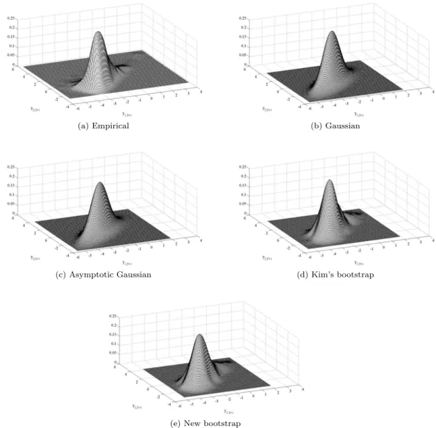
distribution of at is a χ2(4). Panel (a) of Figures 1 and 2 display the joint one-step-ahead and
eight-steps-ahead densities of y1,t and y2,t respectively, which have clear asymmetries, although
more pronounced in the former. After generating a time series of size T = 100, the VAR(2) parameters are estimated by Least Squares (LS). Panel (b) of Figures 1 and 2 plot kernel estimates of the joint density obtained as usual after assuming that the prediction errors are jointly Gaussian
2The same argument can be applied when the interest lies on only a subset of components of Y
t.
For example, if the focus is on the first J components of Yt, the prediction ellipsoid is given by
{YT+h| h YT+h−YbT+h|T i0 C0 CΣb b Y(h)C 0−1C h YT+h−YbT+h|T i < χ2α(J)}, whereC= [IJ 0].
with zero mean and convariance matrix given by (3).3 Comparing panels (a) and (b), it is obvious
that the Gaussian approach fails to capture the asymmetry of the error distribution. It is usual in practice to construct prediction regions fory1,tandy2,t. From the joint Gaussian density plotted
in panel (b) of Figure 1, it is possible to obtain the corresponding 95% one-step-ahead ellipsoids and Bonferroni regions. They are shown in Figure 3 together with a realization ofYT+1. We can
observe that the shape of both regions is not appropriate to construct a satisfactory prediction region for YT+1. Finally, as we may also being interested in forecasting only one variable in
the system, Figure 4 displays the true marginal one-step-ahead density ofy1,t together with the
Gaussian approximation. Once more, it is clear that the Gaussian approach fails to capture the skewness of the prediction density.
Consider first the problem of incorporating the parameter uncertainty. As pointed out above, the MSE in (3) underestimates the true prediction uncertainty and, consequently, they can be inappropriate in small samples sizes. Granted that a good estimator is used, the importance of taking into account the parameter uncertainty could be small in systems consisting in few variables; see Riise and Tjostheim (1984). But, in empirical applications we often found VAR(p) models fitted to large systems; see, for example, Simkins (1995) for a VAR(6) model for a system of 5 macroeconomic variables, Waggoner and Zha (1999) who fit a VAR(13) model to a system of 6 macroeconomic variables, Chow and Choy (2006) who fit a VAR(5) model to a system of 5 variables related with the global electronic system, G´omez and Guerrero (2006) for a VAR(3) model fitted to a system of 6 macroeconomic variables and Chevillon (2009) for a VAR(2) model for a system of 4 macroeconomic variables just to mention a few empirical applications. Addi-tionally, as these examples show, when dealing with real systems of time series, their adequate representation often requires a rather large order p. If the number of variables in the system and/or the number of lags of the model are relatively large, the estimation precision in finite samples could be rather low and predictions based on VAR(p) models with estimated parame-ters may suffer severely from the uncertainty in the parameter estimation. In these cases, it is important to construct prediction intervals and regions that take into account this uncertainty; see, for instance, Schmidt (1977), L¨utkepolh (1991), West (1996), West and McCracken (1998), Sims and Zha (1998, 1999) for existing evidence on the importance of taking into account param-eter uncertainty in unconditional forecasts and Waggoner and Zha (1999) for the same result in conditional forecasts.
3The smoothed density is obtained by applying a Gaussian kernel density estimator with a diagonal bandwidth
To incorporate the parameter uncertainty, L¨utkepolh (1991) suggests approximating the sam-ple distribution of the estimator by its asymptotic distribution density.4 In this case, the MSE
ofYbT+h|T that incorporates the parameter uncertainty can be approximated by
b Σl b Y(h) =ΣbYb(h) + 1 TΩ(b h), (9) where b Ω(h) = h−1 X i=0 h−1 X j=0 trh(Bb0)h−1−iΥb−1Bbh−1−jΥb i b ΨiΣbaΨb0j, (10) withΥ =b ZZ 0
T andBb is the following (N p+ 1)x(N p+ 1) matrix
b B= 1 0 0 ... 0 0 b µ Φb1 Φb2 ... Φbp−1 Φbp 0 IN 0 ... 0 0 ... ... ... ... ... ... 0 0 0 ... IN 0 .
In order to asses the effect of the parameter uncertainty on the MSE given by (9), consider the case of one-step-ahead predictions, i.e. whenh= 1. In this situation,Ω(1) = (b N p+ 1)Σba, and
b Σl b Y(1) can be approximated by b Σl b Y(1) = T +N p+ 1 T Σba.
This expression shows that the contribution of the parameter uncertainty to the one-step-ahead MSE matrix depends on the dimension of the system, N, the VAR order, p, and the sample size, T. As long as N and/or p, or both, are big enough compared to the sample size T, the effect of parameter uncertainty can be substantial. Obviously, as the sample size gets larger then limT→∞T+N pT +1 = 1 and the parameter uncertainty contribution to the MSE in (9) vanishes.
Once the MSE is computed as in (9), the corresponding prediction intervals, ellipsoids and cubes are constructed using the Gaussianity assumption as follows
AIT+h= yn,T+h|yn,T+h∈ b yn,T+h|T ±zα/2σb l n,h , (11)
4Alternatively, some authors propose using Bayesian methods which could be rather complicated from a
com-putational point of view; see, for example, Simkins (1995) and Waggoner and Zha (1999) who need the Gaussianity assumption to derive the likelihood and posterior distribution.
AET+h= n YT+h| h YT+h−YbT+h|T i b Σl b Y(h) −1hY T+h−YbT+h|T i < χ2α(N) o , (12) ACT+h= YT+h|YT+h∈ ∪Nn=1 b yn,T+h|T ±zτbσ l n,h , (13) wherebσl
n,his the square root of thenth diagonal element ofΣbl
b Y(h).
Panel (c) of Figure 1 which plots the density of y1,T+1 and y2,T+1 for the same example as
above constructed assuming that the forecast error are Gaussian with zero mean and covariance matrix given by (9), shows that this density is not very different from that plotted in panel (b) and, obviously, it is not able to capture the asymmetries of the error distribution. Similarly, the joint density of y1,T+8 and y2,T+8 in panel (c) of Figure 2 does not look different from that
in panel (b). The similarity between the standard and the asymptotic densities is even more clear in Figure 3 that plots the elliptical and Bonferroni regions constructed using (12) and (13), respectively. As we can observe they are slightly larger than the standard but still located very close to them. They cannot cope with the lack of symmetry of the prediction error distribution. This similarity could be expected as we are estimating 8 parameters with T = 100. Similar comments deserve Figure 4, where we can observe that the asymptotic marginal density for the first component of the system y1,T+1 only differs from the standard density in the variability,
which is slightly larger in the former.
Note that the asymptotic approximation of the distribution of the LS estimator can be inad-equate in small samples depending on the number of parameters to be estimated and the true distribution of the innovations.
2.2
Bootstrap procedures for prediction intervals and regions
To overcome the limitations of the Gaussian densities described before, Kim (1999, 2001, 2004) and Grigoletto (2005) propose using bootstrap procedures which incorporate the parameter un-certainty even when the sample size is small and do not rely on the Gaussianity assumption.
In order to take into account the conditionality of VAR forecasts on past observations, Kim (1999) proposes to obtain bootstrap replicates of the series based on the following backward recursion
Yt∗=ωb+Λb1Yt∗+1+...+ΛbpYt∗+p+υb ∗
t (14)
where YT∗−i = YT−i for i = 0,1, ..., p−1 are p starting values which coincide with the last
values of the original series, ω,b Λb1, ...,Λbp, are LS estimates of the parameters of the backward
centered and rescaled backward residuals. Then, bootstrap LS estimates of the parameters of the forward representation are obtained by estimating the VAR(p) model in (1) using {Y1∗, ..., YT∗}. Denote these estimates by ˆB∗= (µb∗,Φb1∗, ...,Φb∗p). The bootstrap forecast for periodT+his then
given by
b
YT∗+h|T =bµ∗+Φb∗1YbT∗+h−1|T +...+Φb∗pYbT∗+h−p|T +ba∗T+h (15)
whereba∗T+h are random draws from the empirical distribution function of centered and rescaled forward residuals. Having obtained R bootstrap replicates of YbT∗+h|T, Kim (2001) defines the
bootstrap (1-α)100% prediction interval for thenth variable in the system as follows
KIT+h= n yn,T+h|yn,T+h∈ h q∗Kα 2 , q∗K1−α 2 io (16) where q∗K(γ) is the empiricalγ-quantile of the bootstrap distribution of the nth component of
b
YT∗+h|T approximated by G∗n,K(x) = #(ybn,T∗ +h|T < x)/R. Similarly, Kim (1999) proposes to construct bootstrap prediction ellipsoids with probability content (1−α)100% are given by
KET+h= YT+h| h YT+h−YbT∗+h|T i0 SYKˆ∗(h) −1hY T+h−YbT∗+h|T i < Q∗K (17) where YbT∗+h|T is the sample mean of the R bootstrap replicates Yb
∗(r)
T+h|T and S K
ˆ
Y∗(h) is the
cor-responding sample covariance.5 The quantityQ∗
K in (17) is the (1−α)100% percentile of the
bootstrap distribution of the following quadratic form
h b YT∗+h|T −YbT∗+h|T i0 SYKˆ∗(h) −1h b YT∗+h|T −YbT∗+h|T i . (18)
Furthermore, Kim (1999) proposes using the Bonferroni approximation to obtain prediction cubes with nominal coverage of at least (1-α)100% which are given by
KCT+h= n yn,T+h|yn,T+h∈ ∪Nn=1 h qK∗ τ 2 , q∗K1−τ 2 io (19) whereτ=α/N.6
5Kim (1999) does not explicitly show howSK
ˆ
Y∗(h) should be defined. Alternatively, one can obtainSˆY∗(h) by substituting the parameters in (9) by their bootstrap estimates and computing the average through all bootstrap replicates. By calculating it with the sample covariance or by substituting the bootstrap parameters in the corresponding expressions we get similar results.
6Actually, what Kim (1999) defines as KC is slightly different from (19) as he uses the percentile and percentile-t
methods of Hall (1992). Here we prefer to use the Bonferroni prediction regions in (19) because they are better suited to deal with potential asymmetries of the error distribution; see Hall (1992).
The bootstrap procedure just described is illustrated by considering again the same time series of size T = 100 simulated by model (8). Panel (d) of Figures 1 and 2 plot the joint bootstrap density of y1,T+1 and y2,T+1 and y1,T+8 andy2,T+8 respectively, based on R= 2999 bootstrap
replicates. When comparing these densities with their Gaussian counterparts, it is clear that the bootstrap can reproduce the asymmetry and is much closer to the true density plotted in panel (a) of the same figures. Figure 3 plots the corresponding ellipsoids and cubes defined in (17) and (19). First of all, note that the bootstrap ellipsoid is only slightly larger than the two Gaussian ellipsoids and it is not adequate to represent the shape of the realization of y1,T+1
and y2,T+1 plotted in Figure 2. This is due to the fact the ellipsoid in (17) is still based on a
Gaussian assumption and only differs from the ellipsoids described in the previous subsection in the way the MSE is computed. However, Figure 3 clearly illustrates that when dealing with non-Gaussian prediction errors, the prediction regions constructed from the bootstrap joint densities cannot be based on ellipsoids. An alternative is to use High Density Regions (HDR) proposed by Hyndman (1996) which have also been plotted in Figure 3. These regions are based on kernel estimates of the joint densities as those plotted in Figure 1. Although the shape of these regions seem to be more adequate, they are unfeasible when the dimension of the system is large as, in this case, there are not satisfactory kernel estimators of the bootstrap densities. On the other hand, when the prediction regions are constructed using the Bonferroni approximation, Figure 3 shows that the bootstrap cube is located towards the northeast so it is more adequate than the ellipsoid. This is in fact reflecting that the quantiles of the marginal densities used in (19) can cope with the asymmetries while the ellipsoids use a quadratic form based on the wrong Gaussianity assumption. Finally, Figure 4 displays the marginal one-step-ahead kernel density of
y1,T+1. We observe that it is clearly closer to the true density than its Gaussian counterparts.
Kim (1999) justifies the use of his bootstrap procedure in small samples by suggesting that the asymptotic results of Thombs and Schuchany (1990) can be extended to a multivariate framework. However, the asymptotic validity of the bootstrap procedures based on the backward representa-tion relies on the assumprepresenta-tion of Gaussian innovarepresenta-tions; see Kim (2001). This is due to the fact that the serial independence of the backward errors is needed and this can only be guarantee under the assumption of Gaussian disturbances. Note that alternatively one could use the relationship between the forward and backward residuals and resampling from the former to obtain the latter. However, obtaining the backward representation can be very complicated in VAR(p) models with
large order; see Kim (1997, 1998) for the expression of the backward representation.7
3
A new bootstrap procedure
In this section, we propose an extension of the bootstrap procedure proposed by Pascualet al. (2004a) for univariate ARIMA models, to obtain the joint prediction density ofYT+h in VAR(p)
models. The new bootstrap procedure avoids the backward representation by resampling without fixing the observations of the available sample when incorporating the parameter uncertainty. It is important to note that although the predictions are conditional on the available time series, the sample distribution of the parameter estimator is defined as the distribution through differ-ent replicates; see Harvey (1989) and L¨utkepohl (1991) who argue that the distribution of the predictions based on estimated parameters is obtained as if the sample used for prediction is different from the sample used for estimation. Therefore, using the backward representation is not necessary theoretically and only adds complexity into the bootstrap procedure without any advantage; see Pascualet al. (2004a) for the same arguments in univariate ARIMA models and Rodr´ıguez and Ruiz (2009) for univariate state space models. By avoiding the backward repre-sentation, the new procedure is simpler from a computational point of view, can be implemented in models without such representation and its asymptotic validity can be established without assuming Gaussian errors. In this section, we describe the proposed procedure and prove its asymptotic validity to estimate the joint density of future values of YT+h. We also carry out
Monte Carlo experiments to analyse the performance of prediction intervals constructed from the corresponding marginal bootstrap densities and ellipsoids and cubes constructed from the joint bootstrap density.
3.1
Description of the bootstrap procedure
The new procedure proposed in this paper to obtain the bootstrap prediction density ofYT+h is
similar to that proposed by Kim (1999) but avoiding the backward representation in (14). The algorithm to obtain the bootstrap replicates ofYT+his the following.
Step 1. Estimate by LS the parameters of model (1) and obtain the corresponding vector of
7For the simpler expression of the backward representation in which the lag values of the variables in
(1) are substituted by forward values, Tong and Zhang (2005) and Chan et al. (2006) show that a nec-essary condition for the VAR(p) model to have this backward representation is that the covariance matrices Υ(h) =E[(Yt−E(Yt))(Yt−h−E(Yt))0] are symmetric for allh. This is a very strong restriction not likely to be
residuals defined as in (4). Center and scale the residuals by using the factor [(T−p)/(T−2p)]0.5
recommended by Stine (1987). Denote byFba the empirical distribution function of the centered
and rescaled residuals,Fba(x) =T1
PT
t=11(bat< x) where1(·) is an indicator variable which takes
value 1 if the argument is true.
Step 2. From a set ofpinitial values, sayY∗0={Y−∗p+1, . . . , Y0∗}, construct a bootstrap series
{Y1∗, . . . , YT∗} as follows Yt∗=µb+Φb1Y ∗ t−1+· · ·+ΦbpYt∗−p+ba ∗ t, t= 1, . . . , T, (20) whereba∗
t are independent draws from Fba. ObtainBb∗= (µb∗,Φb∗1, ...,Φb∗p), a bootstrap replicate of
the LS estimates by fitting model (1) to the bootstrap replicate{Y1∗, ..., YT∗}.
Step 3. Forecast using model (1) with the parameters substituted by their bootstrap estimates and fixing the lastpobservations of the original series, as follows
b
YT∗+h|T =µb∗+Φb∗1YbT∗+h−1|T +· · ·+Φb∗pYbT∗+h−p|T +ba∗T+h, (21)
withba∗T+hbeing a random draw fromFba andYbT∗+h=YT+h,h≤0.
Step 4. Repeat steps 1 to 3Rtimes.
Using this procedure, we obtainRbootstrap replicates ofYT+h, denoted by{Yb ∗(1)
T+h|T, ...,Yb ∗(R)
T+h|T}
and their corresponding bootstrap distribution which can be used to delimit prediction intervals, ellipsoids and cubes with appropriate probability content just as before. For instance, if we are interested in thenth component ofYT+h, we can approximate the bootstrap density of the future
value by using{yb∗n,T(1)+h,ybn,T∗(2)+h, ...,by∗n,T(R+)h}, so that a (1-α)100% bootstrap prediction interval for thenth variable is given by
BIT+h={yn,T+k|yn,T+k∈[qB∗ (τ), q ∗
B(1−τ)]} (22)
where qB∗ (τ) = Gn,B∗−1 is the τth percentile of G∗n,B(x) = #(ybn,T∗(b)+k ≤ x)/R. Using similar arguments, we can obtain the following prediction ellipsoids and cubes
BET+h= YT+h| h YT+h−YbT∗+h i0 SB b Y∗(h) −1hY T+h−YbT∗+h i < Q∗B (23) BCT+h= n yn,T+h|yn,T+h∈ ∪Nn=1 h q∗Bτ 2 , q∗B1−τ 2 io (24)
respectively, whereτ =α/N,YbT∗+h|T is the mean of{Yb ∗(1) T+h|T,Yb ∗(2) T+h, ...,Yb ∗(R) T+h}andQ ∗ Bis obtained as in (18).
To illustrate the implementation of the new bootstrap procedure proposed in this paper we consider again the simulated bivariate time series previously described. Panel (e) of Figure 1 displays the kernel estimate of the bootstrap joint density ofy1,T+1 andy2,T+1. It is clear that
it is more adequate to approximate to the true density than Gaussian procedures and similar to the bootstrap procedure proposed by Kim (1999). This is also evident from panel (e) of Figure 2, which looks more alike to that of panel (a) than those plotted in the other panels. Nothing seems to be lost by not using the backward representation. Figure 3 plots the bootstrap cube and elliptical regions obtained from the new bootstrap density. Although the bootstrap densities are very different from the densities obtained by the standard and asymptotic approximations, we cannot observe a big difference in the location between the new bootstrap ellipsoid and those ellipsoids obtained with the alternative procedures. This is due to the fact that first two moments estimates involved in the definition of the ellipsoids do not differ significantly for all the procedures; i.e., all estimate similar centers and dispersions of the future value. For instance, the center of the ellipsoid in Figure 3 is (−2.21,−0.27) for Gaussian alternatives and (−2.21,−0.26) and (−2.19,−0.26) for Kim’s and the new bootstrap approaches, respectively, while the one-step-ahead MSE estimates are given by
b Σ b Y(1) = 0.98 0.79 0.79 0.98 , Σb l b Y(1) = 1.03 0.83 0.83 1.00 , SYKˆ∗(h) = 1.04 0.84 0.84 1.03 andS B ˆ Y∗(h) = 1.09 0.90 0.90 1.08 .
However, we see different locations between the bootstrap cubes and the Gaussian cubes, reflecting the ability of the former to adapt to the asymmetry. Finally, Figure 4 displays the one-step-ahead kernel estimate of the density ofy1,T+1obtained by the new bootstrap which like Kim’s is much
closer to the true density than the Gaussian alternatives. After all, this example suggests that both bootstrap densities resemble better the true density than the traditional procedures. Nevertheless, our bootstrap procedure is much simpler than Kim (1999) and its asymptotic validity can be proven without assuming Gaussianity as it is shown in the next subsection.
3.2
Asymptotic validity
Consider again the stationary VAR(p) model in (1) and assume that there exists ppresample valuesY−p+1,Y−p+2,...,Y0. The error is given by
at(B) =Yt−Φ1Yt−1−...−ΦpYt−p, t= 1, ..., T (25)
where we make explicit that it depends on the unknown parameters contained inB. Denote by
F the distribution of at. Assume that we estimateB by a
√
T-consistent estimator denoted by ˆ
B. The estimated residual is then given by
at(Bb) =Yt−Φb1Yt−1−...−ΦbpYt−p, t= 1, ..., T, (26)
which after being centered they haveF(Bb) as distribution function.8 The asymptotic validity of
the bootstrap depends to a large extend on the approximation given byF( ˆB) toF as the sample sizeTincreases. In particular, Theorem 2.4 of Paparoditis (1996) states thatd2(F( ˆB), F(B))→0
in probability asT →0, whered2is a Mallow’s metric.9
In this paper we consider the LS estimator ˆb = vec(Bb), where vec is the column stacking
operator. The second part of the asymptotic validity relies on the approximation of k bb−b k
given by k bb∗ −bb k. Let’s define the sequence {k I(p) k2} of pN2x1 vectors of constant such
that 0< K1 ≤kI(p) k2≤K2 <∞ andsT =
√
T I(p)0(bb−b). Theorem 3 of Lewis and Reinsel
(1985, p.399) states sT = √ T I(p)0(bb−b) d → N(0, I(p)0(Υ−1 ⊗Σ a)I(p)) in probability where
Υ = PlimZZT0 The bootstrap counterpart of sT is given by s∗T =
√
T I(p)0(bb∗−bb). Denote
the laws of sT and s∗T by ` and `∗, respectively. Theorem 3.2 of Paparoditis (1996, p.284)
establishes thatd2(`, `∗)→ 0 `∗ in probability as T → ∞, where `∗ is conditioned on a given
sampleY. As the convergence in Mallow’s metric implies the convergence of the corresponding random variables thens∗
T d
→N(0, I(p)0(Υ−1⊗Σ
a)I(p)). As far assT ands∗T converge weakly to
the same Gaussian distribution in probability, the bootstrap validity is established. Specifically, Theorem 3.3 of Pararoditis (1996, p.285) sets the asymptotic validity of the Yule Walker estimator of B for the bootstrap procedure, but it still remains valid for any estimator which satisfies
8The asymptotic validity is established for centered residuals, but according to Stine (1987) it remains valid if
they are also rescaled.
9Assume that X and Y are with distribution G
X and GY random variables in RN. The Mallows distance
betweenGX and GY is define asdp(F, G) = inf{E(X−Y)p}p/2, where the minimum is taken over all joint
probability distributionF for (X, Y) such that the marginal distribution ofXandY areGXandGY, respectively.
k Bb−B k= Op(p1/2/T1/2). Consequently, it is valid for the LS estimator considered in this
paper.10
Finally, the asymptotic validity of the bootstrap approximation of the distribution of a future value focuses onYT∗+h|T, which is given by
b
YT∗+h|T =Φb∗0+Φb∗1YbT∗+h−1|T+...+Φb∗pYbT∗+h−p|T +ba∗T+h|T (27)
Theorem. Let {Yt, t=−p+ 1, ...,1,2, ...T} be a realization of a stationary VAR(p) process
{Yt} with E(at) = 0 and E|aitajtaltart| < ∞ for 1 ≤ i, j, l, r ≤ N, ˆB the LS estimator of B
and YbT∗+h|T obtained by following the steps 1 to 4 in the previous subsection. Then, YbT∗+h|T
conditioned on{Yt, t=−p+ 1, ...,1,2, ...T}converges weakly in probability toYT+h asT → ∞.
Proof. Following the arguments in Pascual et al. (2004a), let’s first consider the
one-step-ahead bootstrap future value given by
b YT∗+1|T =Φb∗0+Φb∗1YT+...+Φb∗pYT−p+1+ba∗T+1 (28) Forh= 2 we have b YT∗+2|T =Φb∗0+Φb∗1YbT∗+1|T +...+Φb∗pYT−p+2+ba ∗ T+2 (29)
and replacing theYbT∗+1|T in (28) it follows that b
YT∗+2|T =Φb∗0(1 +Φb1∗) +N1(Bb∗)YT +...+Np(Bb∗)YT−p+1+M1(Bb∗)ba∗T+1+ba∗T+2 (30)
which expresses the bootstrap future values as a function of the given realization{YT−p+1, ..., YT},
the independent random draws ˆa∗T+h and continuous functions of the bootstrap parameter esti-matesBb∗. Proceeding in this way we obtain the following expression
YT∗+h|T =N0(Bb∗) +N1(Bb∗)YT +...+Np(Bb∗)YT−p+1
+M1(Bb∗)ba∗T+1+M2(Bb∗)ba∗T+2+...+ba ∗ T+h
(31)
whereN0mapsBb∗ toN x1,Nj,j= 1, ..., p, andMi,i= 1, ..., h−1, mapsBb∗toN xN matrices.
The functionsNjs andMis are continuous functions and different for each forecast horizon.
Note that N0(Bb∗) and Nj(Bb∗)YT−j+1 are just continuous functions of Bb∗ and YT−j+1 is a 10The VAR process may have an infinite order. In particular, the requirement for the validity of the bootstrap
given value, so that both quantities converge weakly in probability toN0(B) andNj(B)YT−j+1,
respectively. Furthermore,Mi(Bb∗) converges weakly in probability toMi(B) andba ∗
T+j converge
weakly toa∗T+j in probability; therefore, by applying the bootstrap version of Slutsky’s Theorem we obtain thatMi(Bb∗)ba∗T+j
d
→Mi(B)baT+j. Finally, observe thatba∗T+jare independent and thus
all terms in (31) converge weakly in probability. Consequently, YT∗+h|T →d YT+h as T goes to
infinity, in probability.
3.3
Small sample properties
In this subsection, we carry out Monte Carlo experiments to analyse the finite sample properties of the marginal intervals, ellipsoids and cubes constructed by using the new bootstrap procedure proposed in this paper to obtain bootstrap densities. They are compared with those of the Gaussian approximations and the bootstrap procedure based on the backward representation.
The DGP considered all through the experiments is the following bivariate VAR(1) model
y1,t y2,t = + −0.5 0 0.5 0.5 y1,t−1 y2,t−1 + a1,t a2,t (32) where at = (a (1) t , a (2)
t )0 is an independent white noise vector with contemporaneous covariance
matrix given by vecΣa = (1,0.8,0.8,1) 0
. This model have been previously considered by Kim (2001)11. We examine three alternative distributions for a
t, namely, Gaussian, Student-5 and χ2(4). The last two distributions are proposed to capture fat-tailed and asymmetric distributions.
In order to have the covariance matrix described above, the Student-5 and χ2(4) have been
centered and rescaled. The number of Monte Carlo replicates is 1000 and the sample sizes are
T = 25 and 100. We generateF = 3000 future values of of the processYT+h using the assumed
distribution with mean and MSE given by (2) and (3), respectively, which approximate the density of the future value conditional on{Y−p+ 1, ..., Y0, ..., YT}. The parameters are estimated
by LS. Then, the 90%, 95% and 99% marginal prediction intervals for forecast horizons,h, from 1 to 8 are computed for each of the variables in the system by using i) the Gaussian prediction interval without incorporating the parameter uncertainty (GI) in equation (5), ii) the asymptotic (AI) in equation (11), iii) the KI in (16) and, iv) the new bootstrap procedure proposed in
11The model is stationary with roots given by (-2,2). Results for other alternative VAR(1) and VAR(2) models
this paper as in equation (22). The same is done for the prediction regions, whether they are based on the elliptical assumption such as GE in (6), AE in (12), KE in (17) and BE in (23), or the Bonferroni approximations GC in (7), AC in (13), KC in (19) and BC in (24). The number of bootstrap replicates is R = 4999. The number of future values inside the interval and regions is then counted to obtained the empirical coverage of each procedure. We also compute the volume which is given by i) the length of the individual prediction intervals, ii)
V = [π0.5N/Γ(1 + 0.5N)][χ21−α(N)]0.5N{det[Σy(h)−1]}−0.5, where Γ(·) is the gamma function, for
elliptical regions, and (iii) the product of the lengths of the intervals jointly making the Bonferroni approximation. Finally, for individual prediction intervals we calculate the coverage on the left and right sides of the empirical density for the future value.
To compare the alternative prediction densities considered, we rely on an approximation of the Mallows distance based on the following factorization of a joint density
g(y1,T+h, y2,T+h|YT) =g12(y1,T+h,|y2,T+h, YT)∗g2(y2,T+h|YT). (33)
In our setting, we consider the conditional densities ofy1,T+hgiven three different values ofy2,T+h,
which are the 25th, 50th and 75th quantiles of the real density ofy2,T+h; these values are called
byq1,q2 and q3, respectively. To approximate it given a set of realization that characterized a
distribution{Yb
(1)
T+h, ...,Yb
(R)
T+h}, we proceed by considering the realizations on the neighborhood of
these quantiles ofyb2,T+h. For instance, the g12(y1,T+h,|qj, YT) was approximated by the set of
realization satisfying
Cj ={YT+h|YbT+h∈[yb1,T+h, qj]
0±[0, e]0).
Call yC
1,T+h the R12 observations of YbT+h that fulfill that condition.12 Then, the conditional
distribution givenqj isG1|2(x) = #(yb
C
1,T+k ≤x)/R12. The marginal density is obtained just by
considering all the realization in the dimensiony2,T+h, just as beforeG2(x) = #(by (r)
2,T+k ≤x)/R.
Once we have the conditional and marginal distributions, we compute the Mallows distance by computing the difference among 100 quantiles of the distributions involved. Giving a mass 1001 to each quantile, then the Mallows distance between, for instance, the real distribution G2 (or
G12in the case of the conditional distribution) and its bootstrap counterpartG∗2(orG∗12) can be 12Different values of e were proved. Although here we considerer e = 0.1, those values within the limits
approximated as follows d2(G2, G∗2)≈ " 1 100 100 X i=1 ky2(q,T)+h−y∗2,T(q)+hk2 #12
wherey(1q,T)+handy1∗(,Tq)+hare theqth quantile of the real and bootstrap marginal density of the first component. We incorporate this distance calculation exercise within the Monte Carlo simulation framework described above.
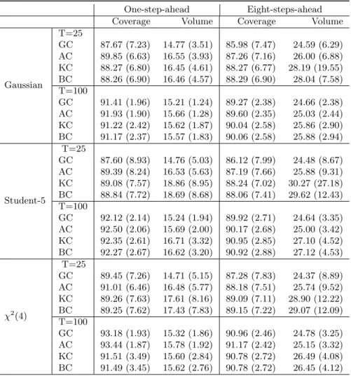
We describe first the results obtained when the objective is the prediction of the marginal distribution of the first variable in the system,y1,T+h. Table 1 reports the Monte Carlo means
and standard deviations of the coverages and lengths of its one-step-ahead and eight-steps-ahead prediction intervals when the nominal coverage is 95%. Table 1 also reports the average of the coverages left out on the right and left of the intervals. When looking at the coverages, Table 1 shows that, regardless of the error distribution, when the sample size is small, T = 25, all intervals have coverages smaller than the nominal; L¨utkepohl (1991) and Kim (1999) also observe undercoverages. In general, the coverage of the GI is the smallest with the AI being slightly closer to the nominal than the bootstrap when the prediction horizon is 1. However, when predicting eight-steps-ahead into the future, the bootstrap intervals are superior to the GI and AI. On the other hand, whenT = 100, the coverages of all intervals are similar irrespective of the distribution and horizon. When looking at the results reported on average lengths, we can observe that they are similar for all procedures and distributions and slightly larger when the horizon is larger. Finally, Table 1 also reports the average coverage on the left and right of the prediction intervals which show that GI and AI are not able to cope with the asymmetry of theχ2(4) error distribution.
These intervals left most observations on just one of their sides. Note that the gains of bootstrap intervals are clearer for longer horizons and when the errors are asymmetric. It is important to remark that although the bootstrap procedure proposed in this paper is much simpler than that proposed by Kim (1999) by avoiding the use of the backward representation, the performance of both prediction intervals is comparable. Therefore, these experiments illustrate that there is not price to pay for not using the backward representation.
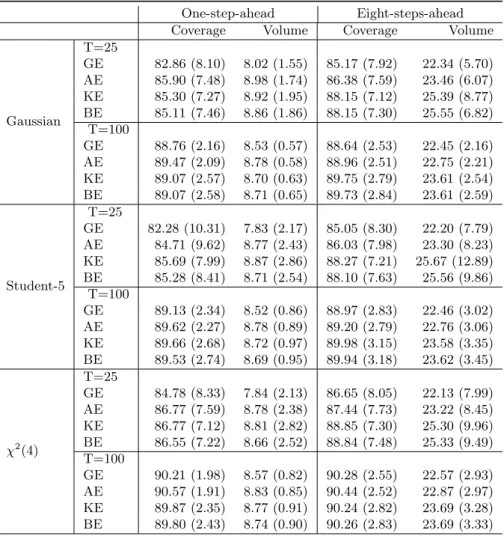
Consider now that the objective is to obtain joint prediction regions that contain the two variables in the system with a given nominal coverage. First, we focus on the performance of the prediction cubes constructed by using the Bonferroni’s approximation. Table 2 reports the corresponding empirical coverages and volumes when the nominal coverage is 90%. The results show that, regardless of the error distribution, when T = 25, the AC has empirical coverage
closer to the nominal than any other procedure. However, when h = 8 the bootstrap regions have better properties. On the other hand, when T = 100 all procedures tend to overestimate the nominal coverage with the bootstrap having coverages closer to the nominal. With respect to volumes, both bootstrap procedures provide regions that are generally larger than the regions obtained by the standard methodology, as they incorporate the parameter uncertainty due to the estimation process. Furthermore, Table 2 shows that the volume associated with non-normal errors are, in general, larger than those corresponding to Gaussian innovations, a feature that is also highlighted by Kim (1999). Note that, as before, there are not differences between the sample performance of the bootstrap procedure propose by Kim (1999) and the simpler one proposed in this paper.
Regarding the performance of the ellipsoidal prediction regions, Table 3 displays similar in-formation to that in Table 2 for a VAR(1) model in (8) for 90% nominal coverage. The main fact to note is that the empirical coverages in Table 2 are below the corresponding coverages in Table 3. This is not surprising since the Bonferroni’s regions provide a cubical approximation with larger volume than ellipsoids, so that it is expected at least the same coverages for the former; see Figure 3. The other features of Table 3 are similar to those commented before for the Bonferroni’s regions.
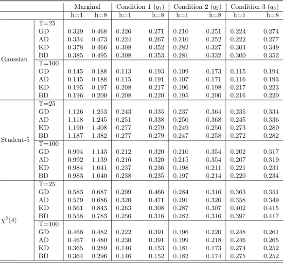
Finally, Table 4 contains mean distances obtained for conditional and marginal densities. Regarding to the marginal density ofy2,T+h, we observe that when the errors are non-Gaussian
and the sample size is medium (T = 100), bootstrap densities perform similarly and better than the alternatives based on Gaussian assumptions, regardless of the forecast horizon. On the other hand, when we consider the conditional densities note that, as expected, in the presence of a Gaussian error and sample size isT = 25, the standard and asymptotic prediction densities are closer to the real than bootstrap densities no matter the forecast horizon. But when the sample size increases toT = 100 and the forecast horizon gets longerh= 8, the differences between the bootstrap densities and those based on a Gaussian assumptions tend to vanish. In case of the error distribution with heavy tails such as the Student-5, the Gaussian and asymptotic procedures do provide good approximations of the real conditional prediction densities, as bootstrap alternatives do, when the sample is either small or medium size and the forecast horizon ish= 1. Furthermore, as the forecast horizon gets longer, bootstrap prediction densities are closer to the real than their alternatives. Finally, when the error isχ2(4) and the sample size isT = 25, bootstrap procedures
perform better for the q1 and q2, regardless of the forecast horizon. When T = 25 and h= 8,
the number of replication when q3 to capture the large asymmetry of that part of the error
distribution; see Figure 1 and Figure 3. On the other hand, when T = 100 bootstrap densities perform clearly better than any other alternative.
After all, the simulations carried out show that the new bootstrap procedure performs bet-ter than traditional methods and does not worse than the procedure based on the backward representation with the advantage that it is easier to implement.
4
Empirical application
In this section, we implement the proposed bootstrap procedure to construct prediction intervals, ellipsoids and cubes for quarterly US inflation (πt), unemployment rate (ut) and GDP growth
(gt) observed quarterly from 1954Q3 to 2010Q4.13 The inflation rates are computed by πt = log(IP It/IP It−1)∗100 where IP I is the US Implicit Price Deflactor. The unemployment is
measured by the civilian unemployment rate14 and, finally, the GDP growth is given by g
t = log(GDPt/GDPt−1)∗100 where GDP is the US Real Gross Domestic Product. The whole sample
period has been split into an estimation sample from 1954Q3 to 2008Q4 (T = 218) and an out-of-sample period from 2009Q1 to 2010Q4. Table 5, which reports some descriptive statistics for the estimation period, shows that for the null of a unit root in the inflation cannot be rejected when using the Dickey-Fuller test; see for instance Stock and Watson (2007) for a discussion of the existence of a unit root in US quarterly IPI inflation. On the other hand, unemployment is stationary at 5% and GDP growth at 1%. Hence a reduce VAR model in which the first difference of inflation (4π) and the current values of unemployment rate and GDP growth rates depend on their lagged values seems to be appropriate for the sample period 1954Q3-2008Q4. On the other hand, the first four columns of Table 5 report the mean, standard deviation, skewness and kurtosis. When considering all the series together the measures of skewness and kurtosis are based on Mardia (1970). It can be observed that all the series are characterized by significant skewness and kurtosis, suggesting non-Gaussian distributions. This is corroborated by the Gaussianity test of Doornik and Hansen (2008) which rejects the null hypothesis of Gaussian series both individually and jointly. To choose the lag-orderp, we use several order selection measures, such as Akaike, Schwarz, Hannan-Quin and the final prediction error criterions. All of them suggest a VAR(3), which is the model finally fitted.
13The data was obtained from the Federal Reserve Bank of St. Louis, webpage: www.stlouisfed.org.
14As the unemployment data is monthly, we chose the value of the last month of each quarter to measure its
The descriptive statistics for the centered and scaled residuals, bat, are displayed in Table 6.
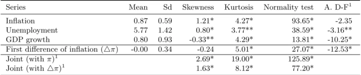
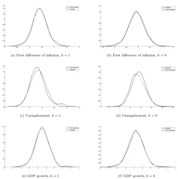
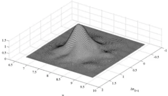
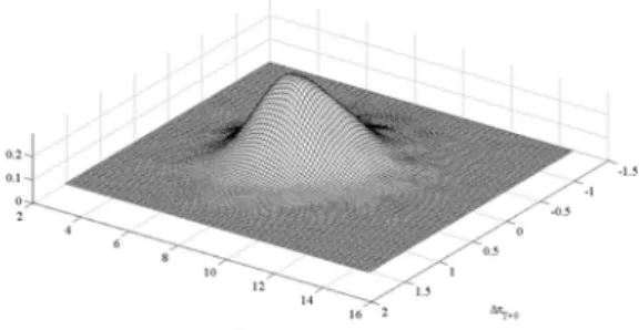
All the estimated residuals have significant excess of kurtosis and Gaussianity is rejected. Overall, this fact suggests that the standard approach to forecasting in the context of VAR models may be misleading when working with these US quarterly series, and therefore the implementation of bootstrap prediction intervals, ellipsoids and cubes is advisable. The estimated VAR(3) model is used to construct the multi-step out-of-sample prediction densities up to horizon 8. Figure 5 plots one-step-ahead and eight-steps-ahead bootstrap marginal prediction densities for each of the variables in the system together with the corresponding Gaussian densities. It can be observed a positive skewness in case of unemployment, just in line with the descriptive statistic of the prediction error. A similar analysis can be done for the multivariate prediction. Figure 6 and 7 plot bivariate one-step and eight-steps-ahead Gaussian and bootstrap densities for the variables considered two by two, respectively. The skewness and the kurtosis of the series individually are also clearly manifested in the shape of the kernel estimates of the bivariate densities. Whenh= 1, this is more evident for first difference of inflation-unemployment and unemployment-GDP growh densities, which are affected by the skewness of unemployment and the kurtosis of inflation rate and unemployment.
Finally, we construct the prediction intervals and regions. Figure 8 plots the multi-step point predictions together with the observed series and the 95% new bootstrap and Gaussian prediction intervals for inflation, unemployment and growth up to horizon 8. Note that as expected the bootstrap prediction intervals are usually larger than those obtained by the standard approach, a fact that is related to the shape of out-of-sample prediction densities. On the other hand, the one-step-ahead density for the unemployment has high kurtosis, positive skewness which is manifested in wider intervals stemming mainly from upper bound. For inflation rate (panel a) and GDP grwoth (panel c), the observed series lie within the 95% prediction bands for both GI and BI. However, for the unemployment series we see that standard method fails to capture the first two out-of-sample values; though the BI captures all the unemployment rates in 2009Q1 and 2010Q4.
Similarly, we construct one-step-ahead and eight-steps-ahead prediction ellipsoids and cubes which are plotted in Figure 9 for the first difference of inflation-unemployment, unemployment-GDP growth and first difference of inflation-unemployment-GDP growth for the Gaussian and the new bootstrap procedures. The point predictors and the observed out-of-sample values for the series are also plotted in Figure 9. Observe that the later values lie outside the GE and GC for the first difference of inflation-unemployment regions, but it is still within the border of the BE and BC. In panel
(b) of Figure 9 we see that something similar occurs for the unemployment-GDP, in which case the observed value lies outside SC but inside the rest of regions; i.e., GE, BC and BE. At last, the out-of-sample value lies inside the cubes and ellipsoids of all procedures for the inflation-GDP growth. Overall, the shape of the regions constructed by each procedure depends on the estimated prediction densities. For instance, in panel (c) of Figure 9 we see that the prediction cube for the unemployment-GDP growth is larger mainly from the unemployment side, which is in part caused by the positive skewness of the unemployment density.
At last, using the out-of-sample observation, we calculate the coverages and volumes of the prediction ellipsoids and cubes obtained using each of the procedures described in this paper. Our strategy is to run a rolling-window estimation for the VAR(3) model starting with data from 1954Q3 to 1966Q4. The sample size is T = 50. Then we construct one-step-ahead elliptical and cubical regions for all the procedures. We count how many real observations belong to the prediction regions constructed and compute their volumes. Table 7 displays the results. With respect to coverage, there are only slight differences between Kim’s and the new bootstrap procedures. However, our method provides smaller regions than the former. Note also that our bootstrap attains better coverage than those approaches based on Gaussian assumptions. After all, the results reported in Table 7 are in line with those obtained with simulated data in the sense that there are no large differences between using the bootstrap procedure proposed in this paper or that proposed by Kim (1999), with the advantage that the our algorithm is simpler from a computational point of view.
5
Conclusions
In this paper we extend the bootstrap procedure proposed by Pascualet al. (2004a) to construct prediction regions in multivariate VAR(p) models. The main attractive of the new bootstrap procedure when compared with alternative bootstrap procedures previously proposed in the lit-erature, is that it does not require the backward representation. As a result, it is possible to prove its asymptotic validity without assuming Gaussian errors. Furthermore, the new procedure can be implemented in multivariate models without a backward representation while its com-putational burden is reduced. We show that the procedure works properly in incorporating the parameter uncertainty and is robust in presence of non-Gaussian errors.
Given its simplicity, the bootstrap procedure proposed in this paper can be easily extended to models with MA components and to cointegrated and non-cointegrated non-stationary systems.
Also, as proposed by Pascualet al. (2004b) in univariate systems, our proposed procedure can also be implemented to obtain prediction intervals for the original observations when a VAR model is fitted to transformed observations; see Ari˜no and Franses (2000) and Bardsen and L¨utkepohl (2011).
Finally, it is often of interest to predict future values of one of the variables in the system con-ditional on particular values of other variables of the system; see, for example, Waggoner and Zha (1999) for a macroeconomic example. The conditional densities can be easily obtained in the con-text of the bootstrap algorithm proposed in this paper by keeping the bootstrap replicatesYb
∗(b)
T+h|T
that satisfy the conditions. Another interesting application of the proposed procedure is the con-struction of confidence intervals for impulse-response functions; see, for example, Killian (1998) for a bootstrap procedure based on the backward representation and Fachin and Bravetti (1996) who proposed a bootstrap alternative which is not. Related with response-impulse functions is the construction of prediction paths; see Staszewska-Bystova (2010) for bootstrap prediction bands based on the backward representation.
Further effort should be directed to the construction of prediction regions. In this sense, it is worth noting that the prediction ellipsoids are only appropriate when the distribution of the future values of the variables in the system is approximately multivariate Gaussian. When the distribution ofYT+h departs from Gaussianity, the quality of such approximation deteriorates.
The Bonferroni’s approximation to the ellipses does provide a better solution capturing the asym-metry of the distribution. However, the shape of the cube could not be appropriate in some cases. Consequently, it would be interesting to give regions that depart either from the elliptical or rect-angular shapes. On the other hand, using HDR as proposed by Hyndman (1996) and applied to GARCH models by Eklund (2005) and more recently by Ter¨arvirta and Zhao (2011), could not be adequate when the number of components in the system is large.
References
[1] Ari˜no, M.A. and P.H. Franses (2000), Forecasting the levels of vector autoregressions log-transformed time series,International Journal of Forecasting, 16, 111-116.
[2] Bardsen, G. and H. L¨utkepolh (2011), Forecasting levels of log variables in vector autore-gressions,International Journal of Forecasting, 27(4), 1108-1115.
[3] Chan, K.-S., L.-H. Ho and H. Tong (2006), A note on time-reversibility of multivariate linear processes,Biometrika,93(1), 221-227.
[4] Chevillon, G. (2009), Multi-step forecasting in emerging economies: An investigation of the South African GDP,International Journal of Forecasting, 25, 602-628.
[5] Chow, H.K. and K.M. Choy (2006), Forecasting the global electronic cycle with leading indicators: A Bayesian VAR approach,International Journal of Forecasting, 22, 301-315. [6] Clements, M.P. and J. Smith (2002), Evaluating multivariate forecast densities: a comparison
of two approaches,International Journal of Forecasting, 18, 397-407.
[7] Diebold, F.X., J. Hahn and A.S. Tay (1999), Multivariate density forecast evaluation and calibration in financial risk management: High-frequency returns on foreign exchange,The Review of Economics and Statistics,81(4), 661-673.
[8] Doornik, J.A. and Hansen, H. (2008), An Omnibus Test for Univariate and Multivariate Normality,Oxford Bulletin of Economics and Statistics,70, 927-939.
[9] Eklund, B. (2005), Estimating confidence regions over bounded domains,Journal Computa-tional Statistics & Data Analysis,49(2), 349-360.
[10] Fachin, S. and L. Bravetti (1996), Asymptotic Normal and Boostrap Inference in Structural VAR Analysis,Journal of Forecasting,15, 329-341.
[11] G´omez, N. and V. Guerrero (2006), Restricted forecasting with VAR models: An analysis of a test for joint compatibility between restrictions and forecasts,International Journal of Forecasting,22, 751-770.
[12] Grigoletto, M. (2005), Bootstrap prediction regions for multivariate autoregressive processes, Statistical Methods and Applications,14, 179-207.
[13] Hall, P. (1992),The bootstrap and Edgeworth expansions, Springer-Verlag, New York. [14] Harvey, A.C. (1989), Forecasting, Structural Time Series Models and the Kalman Filter,
Cambridge University Press.
[15] Hyndman, R.J. (1996), Computing and graphing highest density regions, The American Statistician,50(2), 120-126.
[16] Kilian, L. (1998). Confidence intervals for impulse responses under departures from normality, Econometric Reviews, 17, 1-29.
[17] Kim, J.H. (1997), Relationship between the forward and backward representation of the stationary VAR model, Problem 97.5.2,Econometric Theory, 13, 899-990.
[18] Kim, J.H. (1998), Relationship between the forward and backward representation of the stationary VAR model, Solution 97.5.2,Econometric Theory, 14, 691-693.
[19] Kim, J.H. (1999), Asymptotic and bootstrap prediction regions for Vector Autoregression, International Journal of Forecasting,15, 393-403.
[20] Kim, J.H. (2001), Bootstrap after bootstrap prediction intervals for autoregressive models, Journal of Business & Economic Statistics,19(1), 117-128.
[21] Kim, J.H. (2004), Bias-corrected bootstrap prediction regions for Vector Autoregression, Journal of Forecasting,23, 141-154.
[22] Lewis R. and Reinsel, G.C. (1985), Prediction of multivariate time series by autoregressive model fitting,Journal of Multivariate Analysis,16, 393-411.
[23] L¨utkepolh, H. (1991), Introduction to Multiple Time Series Analysis, 2nd ed., Springer-Verlag, Berlin.
[24] L¨utkepolh, H. (2006), Forecasting with VARMA models, in Elliot, G., C.W.J. Granger and A. Timmerman (eds.),Handbook of Economic Forecasting, Vol. 1, 287-325.
[25] Mardia, K.V. (1970), Measures of multivariate skewness and kurtosis with applications, Biometrika,57(3), 519-530.
[26] Paparoditis, E. (1996). Bootstrapping autoregressivce and moving average parameter esti-mates of infinite order vector autoregressive processes,Journal of Multivariate Analysis,57, 277-296.
[27] Pascual, L., J. Romo, and E. Ruiz (2004a). Bootstrap predictive inference for ARIMA pro-cesses,Journal of Time Series Analysis, 25, 449-465.
[28] Pascual, L., J. Romo, and E. Ruiz (2004b). Bootstrap prediction intervals for power-transformed time series,International Journal of Forecasting, 21(2), 219-235.
[29] Riise, T. and D. Tjostheim (1984), Theory and practice of multivariate ARMA forecasting, Journal of Forecasting,3, 309-317.
[30] Rodr´ıguez A. and Ruiz E. (2009), Bootstrap prediction intervals in statespace models, Jour-nal of Time Series AJour-nalysis, 30(2), 167-178.
[31] Runkle (1987), Vector autoregressions and reality,Journal of Business & Economic Statis-tics,5(4), 437-442.
[32] Schmidt, P. (1977), Some small sample evidence on the distribution of dynamic simulation forecasts,Econometrica,45(4), 997-1005.
[33] Simkins, S. (1995), Forecasting with vector autoregressive (VAR) models subject to business cycle restrictions,International Journal of Forecasting, 11, 569-583.
[34] Sims, C.A. and T. Zha (1998), Error bands for impulse responses, Econometrica, 67(5), 1113-1155.
[35] Sims, C.A. and T. Zha (1999), Bayesian methods for dynamic multivariate models, Interna-tional Economis Review,39, 949-968.
[36] Staszewska-Bystova, A. (2010), Bootstrap prediction bands for forecast paths from vector autoregression models,Journal of Forecasting,doi:10.1002 /for.1205.
[37] Stine, J.H. (1987), Estimating properties of autoregressive forecasts, Journal of Economic Perspectives,15(4), 101-115.