Genome-wide analyses using bead-based microarrays

(1)

Genome-wide analyses using

bead-based microarrays

Mark James Dunning

Jesus College

A dissertation submitted to the University of Cambridge

for the degree of Doctor of Philosophy

Department of Oncology,

Cancer Research Uk, Cambridge Research Institute, Li Ka Shing Centre Robinson Way,

Cambridge, CB2 0RE, United Kingdom. Email: [email protected]

(2)

(3)

This thesis is the result of my own work and includes nothing which is the outcome of work done in collaboration except where specifically indicated in the text.

This thesis does not exceed the specified length limit of 60,000 words as defined by the Clinical Medicine Degree Committee.

This thesis has been typeset in 12pt font using LA_TEX2_ε _{according to the}

specifications defined by the Board of Graduate Studies and the Clinical Medicine Degree Committee.

(4)

Genome-wide analyses using bead-based microarrays

Summary

Mark James Dunning

September 4, 2008 Jesus College

Microarrays are now an established tool for biological research and have

a wide range of applications. In this thesis I investigate the BeadArray

microarray technology developed by Illumina. The design of this technology is unique and gives rise to many computational and statistical challenges. However, I show how knowledge from other microarray technologies can be used to our advantage.

I describe thebeadarraysoftware package, which is now used by researchers

around the world. The development of this software was motivated by the fact that Illumina’s software (BeadStudio) gives a summarised view of Illu-mina data and does not gives users any control over several processing steps that were found to be crucial for other microarray technologies. A main

feature of beadarray is the ability to access raw data. The advantages of

such data include the ability to perform more detailed quality assessment and greater control over the analysis at all stages. The analysis of a con-trol experiment shows that the processing steps used in BeadStudio can be improved. In particular, utilising variances calculated from the raw data can increase the ability to detect genes which have different expression lev-els between samples, a common goal for microarray studies. The data from the control experiment are made available for other researchers to use and validate their own analysis methods.

One issue discovered during the analysis of the control experiment was that only half of the intended genes could be reliably measured due to prob-lems in the design of the probes targetting particular genes. By considering a large set of publicly available Illumina arrays, I show how such unreliable measurements can affect the analysis of Illumina data. I also show how poten-tial problems can be identified in advance of an experiment and incorporated into an analysis pipeline.

(5)

Preface

This thesis describes work undertaken in the Computational Biology group in the Department of Oncology at the University of Cambridge between Jan-uary 2005 and June 2008. This section of the thesis proved one of the most difficult to write because there are so many people to which I am grateful! During this time I had the good fortune to work on many interesting topics and be surrounded by so many talented individuals that made working in the group thoroughly enjoyable. I would firstly like to thank my supervisor,

Si-mon Tavar´e for his patient support and guidance over the past 3 years. The

other members of the group have helped me in many ways over the years with scientific discussions and moral support. I am very grateful to Natalie Thorne, Matthew Ritchie, Andy Lynch, Nuno Barbosa-Morais and Christina Curtis for their constructive comments on my work and it has been a real pleasure collaborating with them. My fellow students in the lab have also contributed greatly to the stimulating environment, and I am sure each one has an exciting future ahead of them. I am also grateful to the training I received at University of York and my supervisors Jason Levesley and Garib Murshudov for their encouragement to take up this PhD.

There are many individuals that provided much-needed support outside the world of bioinformatics. In particular my housemates in Malcolm Street (past and present), and especially to Anna Julian for her support over the past few months. I am also quite fortunate to keep in close contact with several school-friends and it is always a real pleasure to meet up and hear about their achievements.

Finally, special thanks must be given to my parents for their continued encouragement throughout the years, and also to my grandparents who are sadly not here to witness the completion of this work.

(6)

List of Tables

2.1 Summary of GEO datasets derived using Human6 chips. For

each entry we list the citation, number of arrays used, type of filtering applied to the data, and normalisation method ap-plied. All datasets had preliminary analysis done using

Bead-Studio. . . 37

5.1 Table showing the reannotation of the probes sequences for all

non-spikes in the spike-in experiment. The 23,983 probes on Strip 1 and 22,022 probes on Strip 2 are divided into categories

(see page 82) describing various annotation problems. . . 94

6.1 Results of reannotation of the Illumina Human6 Version 1

platform. The 26,091 probes on Strip 1 and 21,198 probes on Strip 2 are divided into categories describing various anno-tation problems. “Good” denotes probes that had a complete genomic match to the exonic region of a known transcript. . . 117

(11)

List of Figures

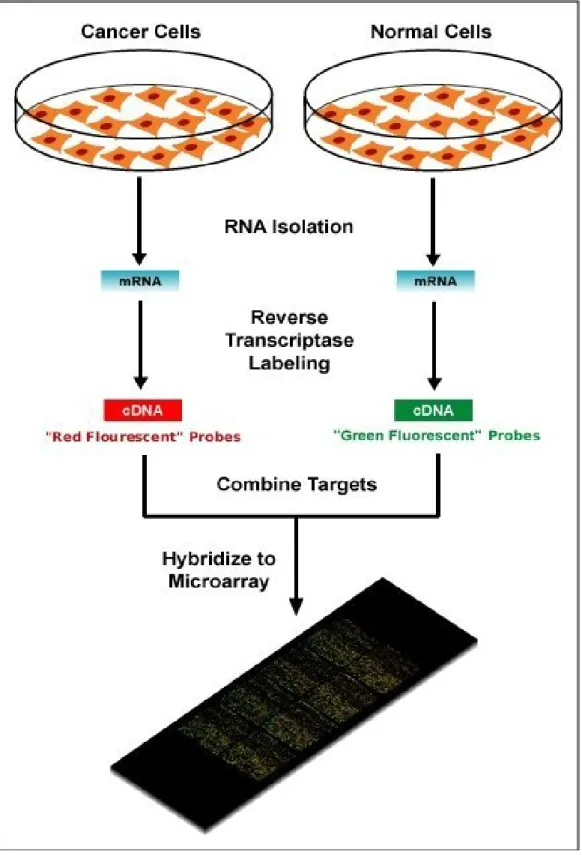
1.1 This public domain image shows a schematic diagram of a

typical two-colour microarray experiment to compare DNA

from a cancer cell to that of a normal cell. . . 5

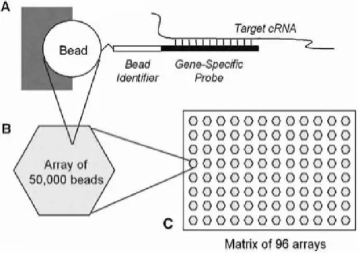
1.2 Constructing an Illumina “array of arrays”, in this case a SAM:

A) Each bead sits in a pre-created well on the surface of an

array and has probes attached that are complementary to a particular genomic sequence of interest. In this figure, only one sequence is shown, although the bead will have thousands of these sequences attached. The bead also has a unique identifier

sequence which is used for decoding purposes. B) Each array

has around 50,000 beads that are randomly arranged. Around 1,500 distinct bead types are represented around 30 times each.

C) A matrix of 96 arrays is constructed, each array being

uniquely prepared and thus having a different arrangement of

(12)

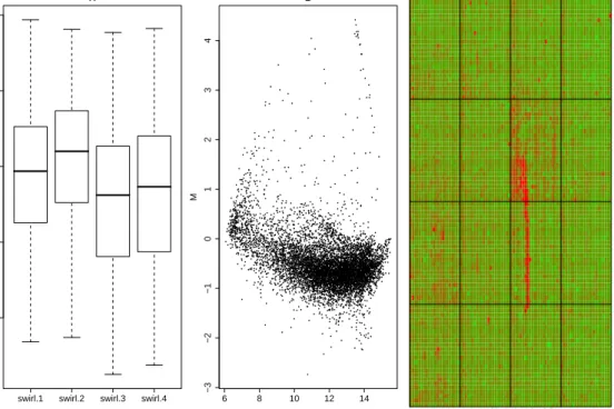
1.3 QA plots for a two-colour microarray experiment provided

with the limma user guide. A) Boxplots of the red foreground

for four arrays in the experiment, showing the median values and inter-quartile range of each array. Ideally, the foreground measured on each array should have roughly similar distri-butions. However, the intensities on the first two arrays are generally higher. B) An MA-plot for the red and green chan-nels for a particular array, with the log-ratio (M) plotted on the y-axis and log-average (A) on the x-axis. We would expect that most probes are not DE, and should therefore be centred

alongM = 0. In this example, most points are away from this

line and adjustment is required to remove this trend. C) Im-ageplot of the log-ratios for a particular array, with green and red representing low and high intensities respectively. Ideally, a random scattering of colours should be seen. However, a red streak is seen in the 3rd column of the array. Spots affected by this artefact have log-ratios that are systematically higher and might not be attributed to differences in the biological

conditions being studied. . . 11

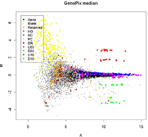
2.1 Illustrative example of the “fanning effect” for microarray data.

This MA-plot compares two replicates of the same biological

sample, and hence no differential expression (M = 0) should

be expected. However, for A<7, the M-values are seen to have

a wide range of values. The coloured spots indicate control

probes on the array. Figure courtesy of Gordon Smyth. . . 19

2.2 A cartoon representation of a bead in the direct hybridisation

assay. Each bead has an address sequence attached for decod-ing purposes and a 50 base sequence specific to each bead type. The probe sequence is fluorescently labelled and designed to hybridise to a particular genomic sequence. Note that the di-agram is not shown to scale and many thousands of sequences

(13)

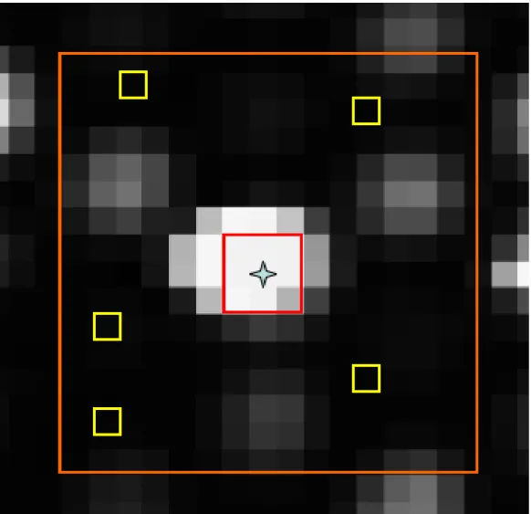
2.3 Diagram of the steps used for calculating the foreground and background of a bead. Using the coordinates determined dur-ing the decoddur-ing step, a centre for the bead is known, indicated by a cross in this figure. The intensities of the four closest

pix-els in a 3×3 square around the centre (red square) are then

used in a weighted average to calculate the foreground. The

five dimmest pixels within a 17×17 square around the bead

centre (orange square) are averaged to give the background in-tensities. In this figure, the five dimmest pixels are indicated by the yellow squares. Figure courtesy of Dr. Matthew Ritchie. 32

3.1 An overview of the beadarray software and the various tasks

it can perform compared to BeadStudio. The software can be used to analyse either bead-level data or data exported from BeadStudio, although availability of bead-level data allows a

more flexible analysis. . . 46

4.1 Foreground (A), background (B) and background corrected

(C) intensities of all beads in the BioC07 dataset. Arrays

are coloured separately for Sample A (blue) and Sample B (red). The foreground intensities are seen to be consistent across the dataset, with the exception of arrays 1 and 6 which are generally have higher intensity. The background intensity

has extremely low variability on all arrays. . . 60

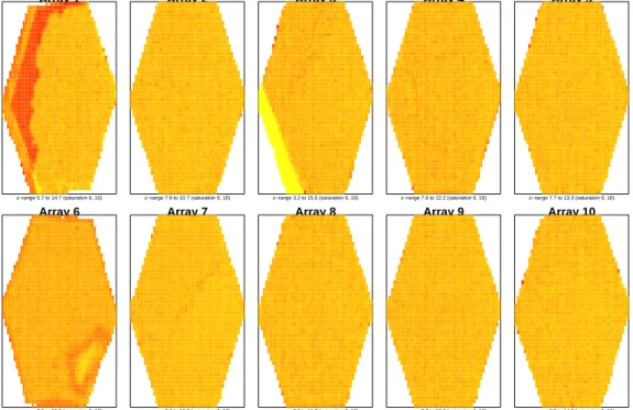
4.2 Imageplots of foreground intensity for the BioC07 dataset,

with replicates of sample A in the top row, and sample B in the bottom row. Red and yellow denote high and low in-tensity regions respectively. Clear spatial artefacts can be seen

for arrays 1, 3 and 6. . . 62

4.3 The locations of beads that are found to be outliers on arrays

1, 3 and 6, which were seen to have spatial artefacts in Figure 4.2. With the exception of Array 3, the locations of outliers correspond well with the spatial artefacts seen by eye. The outlier removal method implemented by Illumina was used, which excludes beads using a cut-off of 3 MADs from the

(14)

4.4 An overview of the BioC07 dataset after summarising the bead-level data. The summarised expression levels for all ar-rays are seen to be in good agreement, although arar-rays 1 and 6 have slightly higher medians. Array 1 also has fewer bead types with extreme high intensities. The number of beads af-ter outlier removal are also shown for all arrays in the BioC07 dataset. The average number of beads for a bead type in a given array is generally around 30, although arrays 1, 3 and 6 have lower numbers of replicates. No bead type on any array

has fewer than 10 replicates. . . 65

4.5 MA plots constructed using selected replicates of Sample A

(top row) and replicates of Sample B (bottom row). Compar-ing Array 1 to arrays that have the same biological sample hybridised yields many genes with log-ratios away from 0 in a non-linear fashion. This trend is not seen for other com-parisons of Sample A. The log-ratios generated using Array 6 are more variable than other comparisons of this sample and also systematically greater than 0. However there are many

normalisation schemes that might correct for this. . . 66

4.6 Comparison of the volcano plots produced for a differential

expression analysis involving all arrays (left) and with Array 1 removed (right). The y-axis shows a measure of evidence for differential expression (log-odds) and the x-axis shows the estimated coefficients from the linear model. Red dots indicate genes with positive log-odds (roughly corresponding to greater than 50% chance of being DE) in the analysis that excludes Array 1. Removal of Array 1 from the analysis is seen to

improve our ability to detect DE genes. . . 68

4.7 The percentage of outliers for a random selection of 200

ar-rays from the HapMap dataset, with outliers below and above the median shown in blue and red respectively. On the left, outliers were removed on the unlogged scale using a 3 MAD

cut-off, and on the right a log2 transformation was applied

prior to removing outliers. Without applying a log2

transfor-mation, we find many more outliers above the median than below, whereas we get a more even distribution of outliers

(15)

4.8 An overview of the overall array intensities for the HapMap dataset. The median intensities were calculated for each of the 1400 arrays and plotted according to which SAM (indicated by a 7 digit number) the arrays belong to. Clear differences

are seen between the chips. . . 71

5.1 Raw foreground and background intensities for each strip on

a typical BeadChip. Each BeadArray is made up of two strips (colour-coded) on the chip surface. The consistency of fore-ground and backfore-ground signals between arrays is evident from this plot, as is the tendency for beads from Strip 1 to have

higher intensities than those from Strip 2. . . 84

5.2 The average bias (A) and log2 variance (B) versus percentage

of simulated outliers plotted for each summary method. In panel A, we see that Illumina’s summary method can han-dle up to about 30% of saturated intensities before the bias starts to increase dramatically. The trimmed mean breaks down much earlier, at around 5%. The median is comparable to Illumina’s method. Similar trends can be noticed in the

variance (B). . . 85

5.3 Boxplots of the means (A) and variances (B) for the 33 spikes

on all arrays in the experiment after outlier removal. The box-plots are arranged in decreasing order of spike concentration, with different background correction methods labeled in dif-ferent colours. The no background adjustment option shows dramatic attenuation in signal, which begins at a higher

(16)

5.4 MA-plots comparing the bead-summary values for one array with spike concentration 3pM to an array with spike concentra-tion 1pM. An increased density of points is indicated by darker shades of blue. Red points highlight the spike genes. The

hor-izontal line at M=1.73 represents the intended log-ratio for

the spike genes, and the line at M=0 is the desired level for

the remaining non-spikes. Each panel shows the data pro-cessed using different background correction methods. Panel A shows the data with no background adjustment, while in panel B local background has been subtracted and in panel C the data have been background subtracted and background normalised. When the data are background subtracted, the

range of M and A-values increases and the spike genes are

closer to the true value than for the non-adjusted data. BGN

(see page 31) produces the most variable M-values and

over-estimates theM-values for the spikes. . . 89

5.5 The distribution of background subtracted and summarised

intensities for 50 negative controls across all arrays in the ex-periment, ordered by increasing median. Each control is a bead type with a random sequence attached that should not hybridise to any target in the genome. Despite this, some con-trols clearly appear to show consistently higher intensity than

others. . . 90

5.6 Boxplots of the log-odds scores (A) and log-ratios (B) obtained

after fitting a linear model to all genes across all arrays in the spike experiment and making contrasts between 3pM and 1pM. A separate box is shown for each background correction

method with a standard linear model and a weighted log2

anal-ysis. Two separate boxplots are shown for each method and weighting scheme to indicate the log-odds scores for the spikes

(bold colours) and non-spikes (transparent). The weighted

log2 analysis improves the log-odds scores for the spikes

with-out increasing the log-odds for the non-spikes, which repre-sents an increase in power to detect true differential expres-sion. In panel B, we show that the log-ratios for the spikes are under-estimated when the data are not background adjusted,

whereas the background subtracted and normexp processed

data recover values much closer to the true log fold-change

(17)

5.7 The log2 intensities for the 33 spikes on each array estimated

using the linear model. Each spike is indicated by a different colour and line. Despite being added at the same concentra-tion, consistent differences are seen between the spikes, for

example, ela 2 consistently has the lowest intensity. . . 93

5.8 Boxplots of all bead types intensities on an arbitrary Strip 1

array grouped according to the reannotation of the probe se-quence assigned to the bead type. Bead types with reliable annotation (the “Good” category) are seen to have higher

in-tensity compared to others. . . 96

5.9 Normalised log2 intensities for all non-spikes on Strip 1 of a

particular array in the experiment grouped according to the number of As, Ts, Gs or Cs in the sequence for the probe.

The normalised log2 intensities and bead type variances are

also shown in terms of GC content. The width of each box is proportional to the number of observations. Probes with higher GC content are shown to have higher intensity on av-erage and a lower variance. Finally, estimated effect sizes are shown for each base position relative to having a T at that position. The normalised intensities are seen to be higher if a G or C is present at the first base in the sequence and have a

lower variance. However, no other systematic trend is seen. . . 97

5.10 The log-odds ranking of all non-spikes on Strip 1 in the con-trast between 3pM and 1pM aggregated according to the GC content of each probe. Probes with a GC content of 18-21 are generally ranked higher in the list. The width of each box is

proportional to the number of observations. . . 98

5.11 Demonstrating the VST transformation for an array in the spike-in experiment. A) The undesirable relationship between bead type means and standard deviations is shown. The linear

fit shown in green is used to estimate the parametersc1andc2.

B) Comparison of VST and log2 transformed values for this

array with the green line representing VST = log2. Figure

(18)

5.12 Here, we show the MA-plots for an array with spikes at con-centration 3pM against spikes at concon-centration 1pM. In the

top row, the arrays were transformed with a log2

transforma-tion or VST. In the bottom row, the arrays were background normalised before transformation. In all plots, red dots mark the values for the spike probes and the dotted lines indicate the predicted log fold-change of spikes (1.73) and non-spikes (0) respectively. . . 107 5.13 Comparison of spike log-odds obtained for a particular

con-trast in the linear model fitted to the entire spike-in experi-ment of 48 arrays. On the left we show the difference between the log-odds obtained after VST and the log-odds obtained

af-ter a log2 transformation. On the right, we show the difference

between VST and a linear model incorporating log2 variances

as weights. In the top panels, we show six independent con-trasts with the closest spike concentrations. The bottom panel shows six independent contrasts from the same linear model, but chosen to provide a range in anticipated log-ratios (the finer differences being to the right of the panel). In all cases, a positive value indicates greater log-odds obtained (i.e., more

evidence for differential expression) after VST. . . 109

5.14 Comparison of spike log-odds obtained for a particular con-trast in the linear model fitted to the 8 arrays involved in that contrast. On the left we show the difference between the log-odds obtained after VST and the log-log-odds obtained after a

log2 transformation. On the right, we show the difference

be-tween VST and a linear model incorporating log2 variances as

weights. In the top panels, we show six independent contrasts with the closest spike concentrations. The bottom panel shows six independent contrasts chosen to provide a range in antici-pated log-ratios (the finer differences being to the right of the panel). In all cases, a positive value indicates greater log-odds obtained (i.e., more evidence for differential expression) after

(19)

6.1 Two different views of non-normalised Illumina data from the MAQC study. In A, we show data from one location. One array was removed during quality assessment by the MAQC so in total there are 19 arrays with 48,000 observations each. In B, the same arrays are divided into the probes found on Strip 1 and Strip 2. Similar boxplots were seen for all three

locations. . . 119

6.2 For different filtering methods (see Section 6.2.3) we show the

percentage of genes belonging to Strip 1 and Strip 2 and dif-ferent annotation categories retained by the filter. . . 121

6.3 Average ranks of probes across all Illumina Human6 arrays in

GEO. A) shows the average ranks of probes on Strip 1 versus probes on Strip 2. Probes on Strip 1 (roughly equivalent to the lower-density Human8 arrays) are found to be ranked higher than those on Strip 2. In B) the probes on Strip 1 are split into different annotation categories. . . 122

6.4 Representing the composition of ranked lists of genes obtained

from the MAQC dataset after a differential expression analy-sis. Separate curves are shown for each pairwise contrast of samples. For the linear model fitted to all probes (Fit 1), we show the proportion of Strip 1 or Strip 2 probes encountered along the length of the gene list. For the linear model fitted to probes from Strip 1 only (Fit 2), we show the composition of the gene list in terms of the annotation categories. . . 126

6.5 Improvements to the detection of DE genes by filtering. On the

left, the number of significant findings (after multiple testing correction) for Strip 1 probes using Fit 1 and Fit 2 are shown. For all the contrasts, the number of significant probes is greater using Fit 2. On the right, the number of probes with good annotation is shown under Fit 1 and Fit 2. Fit 3 is also seen

to increase the number of significant findings. . . 128

6.6 Screenshots of the BLAT search for probe GI 42657060-S. The

top screen just some of the locations that the probe matched to. The bottom screen shows the genomic location of the top match. The probe sequence is seen to be outside any RefSeq genes and matching a region of the genome with a long-term repeat item. . . 131

(20)

6.7 The rank of probe GI 42657060-S across all Illumina Human6 Version 1 arrays in GEO. It can be seen that regardless of sample or processing method, the probe is generally among the highest ranked probes on an array. The different colours represent the different datasets. . . 132 C.1 Modified TIFF images for arrays 1, 3 and 6 from the BioC07

(21)

List of abbreviations

BGN - Background normalisation used by Illumina to calibrate arrays

to the same baseline.

BLAT - Basic Local Alignment Tool.

cDNA - Complementary DNA

DE - Differentially expressed.

DNA - Deoxyribonucleic acid

Human6 - A chip manufactured by Illumina to interrogate 48,000 genes

on 6 human samples.

Human8 - A chip manufactured by Illumina to interrogate 22,000 genes

on 8 human samples.

limma - Linear models for microarrays R package

Mouse6 - A chip manufactured by Illumina to interrogate 48,000 genes

on 6 mouse samples.

mRNA - Messenger ribonucleic acid

normexp - Normal-exponential convolution method used for background

correction.

RefSeq - Reference sequence database.

SAM - Sentrix Array Matrx format used by Illumina that has 96 arrays

in a 8 × 12 matrix.

QA - Quality assessment.

(22)

Chapter 1 Introduction

This chapter gives a brief introduction to the use of microarrays for medical research and motivates the need for statistical and computational tools to deal with the vast amounts of data generated by such devices. I will also in-troduce the technology behind bead-based microarrays, which are the subject of investigation in this thesis.

1.1 Overview of DNA and RNA

Deoxyribonucleic acid (DNA) encodes the information required for the devel-opment and function of a living organism. The structure of DNA is remark-ably simple, being formed of a long chain of smaller units (nucleotides) joined together. Each nucleotide can have one of four bases attached; Adenine (A), Cytosine (C) Thymine (T) or Guanine (G). The order in which these bases occur in a DNA molecule is known as the DNA sequence.

Structurally, a DNA molecule takes the form of a double helix formed by two strands of DNA. This structure is held together by strong hydrogen bonds between the two strands. The bonding takes place in such a way that A base-pairs with a T base in the opposite strand, whereas C base-pairs with G. This is known as the base complementarity property of DNA and effec-tively means that the sequence of one strand can be determined by the other, a fact that is exploited during DNA replication.

The entire DNA sequence of an organism is known as its genome. The human genome is estimated to have 3.3 billion bases and can be found in the

(23)

nucleus of every cell in the body. Rather than being one long DNA molecule, a genome is divided into continuous regions of DNA known as chromosomes. There are 24 chromosomes in the human genome, which are numbered 1 to 22 plus the sex chromosomes, X and Y. Most “healthy” cells in the human body contain 46 chromosomes; two copies of chromosomes 1 to 22 (one copy of the chromosome inherited from either parent) and either an X and Y chro-mosome (for males) or two copies of the X chrochro-mosome (for females). Each chromosome is divided into stretches of DNA called genes, which encode the instructions to produce a particular protein. The estimated number of genes in the entire human genome is between 25,000 and 30,000. However, rather than being one continuous sequence of genes, there are many gaps in the chromosome that are not genes and hence do not code for proteins. In fact,

only an estimated 5−10% of our genome is used to code for proteins. The

purpose of remaining “junk DNA” is a source of much debate, but increas-ingly is considered to have regulatory function.

The instructions encoded in the DNA sequence are stored in the nucleus and must be transported to the cytoplasm, where specialised molecules called ribosomes help produce the required proteins. However, the DNA sequence itself is too valuable to be transported. Therefore, sections of DNA are copied

(transcribed) into temporary messenger RNA (mRNA) molecules that

con-tain the same information as DNA, but in a slightly different form. The main differences are that mRNA is single-stranded, degrades quickly and has a Uracil (U) base instead of a T. The entire sequence of each gene is tran-scribed, even though not all parts of the sequence take part in coding for proteins. Such non-coding regions, known as introns, are removed by splic-ing before the process of translation starts. Translation uses mRNA as a template to assemble previously synthesised amino acids in the correct order to make particular proteins, with groups of 3 successive bases used to specify the amino acid located in that position in the chain.

Although each cell contains copies of the same genome, the cell will re-quire different amounts and combinations of proteins in order to perform its function within the body. Therefore, the genes that control the production of these proteins may be turned on or off to varying degrees. These changes confer unique properties to each cell type. The expression level of a gene refers to the amount of mRNA that is made from the DNA template and

(24)

subsequently translated into protein.

Given that the genome contains the complete set of instructions required to develop and maintain a living organism, it is little wonder that medi-cal research has invested heavily in methods for studying the genome, and in particular the regulation of gene expression. Being able to understand the differences between healthy and diseased cells, and the mechanisms that bring about these differences is of chief importance. For example, the growth of a cell is tightly regulated by proto-oncogenes which keep a cell dividing and growing, whilst tumour-suppressor genes bring about the death of a cell when required. Clearly, disruptions to the normal activity of these genes could have serious implications for the development of cells, with diseases such as cancer associated with cells that have grown out of control.

In the next section, I describe a popular experimental technique for de-termining the expression level of a large set of genes in a given sample. The data generated by these experiments require careful processing and statistical analysis in order to draw valid biological conclusions. These issues will also be addressed later in this chapter.

1.2 Gene expression microarrays

A microarray (sometimes referred to as an array) is a device for

simultane-ously measuring the expression level of thousands of genes. The technology makes use of the base-complementarity property of DNA and the fact that single-stranded mRNA is produced in order for a particular gene to be ex-pressed. Thus, by measuring the amount of mRNA we can infer the expres-sion level of the gene.

Microarrays are typically constructed by attaching single-stranded DNA

sequences, known as probes, to a surface such as a glass slide. Each probe is

complementary to the DNA sequence of a particular gene of interest and is placed in spots (or features) at pre-defined locations. Single-stranded mRNA

from a sample of interest (called the target) is isolated, converted into

single-stranded DNA (cDNA) and then transcribed into cRNA. These cRNA are then fluorescently labelled, and exposed to the microarray surface. The tar-get RNA then binds (hybridises) to its complementary probe sequence on the

(25)

microarray, whereas non-complementary sequences should fail to hybridise. The amount of fluorescence observed at each feature can therefore be used to determine the level of expression for each of the genes represented on the

array. In the earliest microarrays (_Schena et al., 1995), each feature on

the array corresponded to a different gene of interest. However, subsequent developments in microarray production have allowed the same gene to be rep-resented multiple times, thus providing more reliable expression estimates.

Two-colour microarrays are used to compare two samples (e.g. cancer and normal cells) on the same microarray. The RNA from the two samples is extracted separately and fluorescently labelled with different dyes, usually red and green. Therefore, after hybridisation, each feature is a mixture of red and green fluorescence. A completely red or green feature indicates that a particular gene is expressed in one sample, but not the other. In practice, the mixture of red and green observed at each feature is not so clear-cut and statistical methods are required to quantify the contribution of each colour, as described later. A “differential expression” analysis aims to find genes that have significantly different expression levels between different conditions un-der investigation. Such genes are said to be differentially expressed (DE). See Figure 1.1 for an illustration of a typical two-colour microarray experiment.

Microarrays have become an invaluable tool for medical research (

Alli-son et al., 2006) and provide a wealth of data that was previously

unob-tainable. The production of microarrays is a rapidly growing industry, with many companies supplying variations of the technology for a wide range of applications. Each company has a different method of manufacturing mi-croarrays, the major differences being the production of the probe sequences used and the method of depositing these sequences onto the array surface. For instance, different length probe sequences (usually measured in the num-ber of base-pairs) can be used as well as mRNA or cDNA probes, rather than the cRNA probes described above.

Single-channel microrrays can also be produced to measure the absolute expression level of every gene of interest in a given sample. Therefore, the fluorescence of each feature is a measure of the expression level of a particu-lar gene. Until recently, arguably the most popuparticu-lar single-channel microarray

(26)

Figure 1.1: This public domain image shows a schematic diagram of a typical two-colour microarray experiment to compare DNA from a cancer cell to that

(27)

use 25 base-pair probes that are synthesised on the array surface. Each gene of interest is interrogated by a collection of 11-20 probe pairs, known as a

probe set. The expression level for a gene is then derived by combining all measurements from a particular probe set.

Additionally, microarrays are manufactured for applications other than gene expression. For instance, microarrays can be used to interrogate regions of the genome where differences in a single base (Single Nucleotide Polymor-phisms, or SNPs for short) are observed in a population, or regions where long stretches of DNA are gained or lost (Copy Number Variation or CNV). Adaptations of these technologies can also investigate changes to the genome, such as methylation, that alter the structure of DNA but not the sequence, and the locations where proteins might bind to the genome in order to en-courage or impede expression

1.3 Illumina bead-based microarrays

In this thesis, I will concentrate on the BeadArray microarray technology developed by Illumina, which is becoming widely used and offers many po-tential benefits over other technologies. Rather than attaching probes onto a microarray at known locations, BeadArrays are self-assembling arrays of minute beads with probes attached. Each array is produced separately by exposing an array surface (either a glass slide or fibre-optic bundle) to a large collection of pre-prepared beads. This causes the beads to be randomly

sam-pled and assembled into wells on the surface of the array (_Fan et al., 2006).

A specific DNA sequence is assigned to each bead type, which is replicated

on about 30 beads on an array. Each bead is 3 microns in diameter and has many thousands of copies of the same probe sequence. Both the number and location of the replicates for the same bead type are random on an array (Kuhnet al., 2004). Therefore, an extra address sequence (anIllumiCode) is

attached to each bead for decoding (Gundersonet al., 2004), with beads of

the same type also having the same IllumiCode. Each IllumiCode is designed to hybridise in a predictable way to a series of specially designed dye-labelled sequences. After each hybridisation, each bead is assigned to one of two states (e.g. red or green) depending on the amount of hybridisation. Thus, after a number of such hybridisations, a binary sequence is determined for

(28)

each bead. This binary sequence should then uniquely correspond to the predicted response of an IllumiCode. These decoding hybrisidations are per-formed by Illumina, with the guarantee that no array will be supplied to the user with a bead type that has less than five replicates.

Along with the high degree of replication within an array, Illumina also offer the capability of processing BeadArrays in parallel, making this tech-nology desirable for high-throughput experiments. A Sentrix BeadChip is a glass slide (chip) that allows a very high number of observations to be made for a particular sample. Depending on the configuration of the chip, between 1 and 16 samples can be processed simultaneously with tens of thousands of genes profiled per sample. A more detailed description of this chip tech-nology is given in Chapter 2. The Sentrix Array Matrix (SAM) contains 96 arrays, each of which is a hexagonal fibre-optic bundle with approximately 50,000 beads and around 1,500 distinct bead types. Thus, 96 samples can be interrogated simultaneously on a single SAM. See Figure 1.2 for a summary of how these arrays are constructed.

1.4 Pre-processing and analysis of

microar-ray data

Despite differences in array production, the common goals of any gene expres-sion study are roughly the same and one has to deal with similar statistical issues when analysing microarray data. For instance, the intensities of the features on a microarray are influenced by many sources of noise and re-peated measurements made on different microarrays may also appear to dis-agree. Therefore, a number of data-cleaning, or pre-processing steps, must take place before being able to draw valid biological conclusions from a

mi-croarray experiment (Quackenbush, 2002; Smyth et al., 2003; Allison

et al., 2006).

These steps are well-understood for established microarray technologies (e.g. Affymetrix or older two-colour arrays). However, at the start of my PhD there was little coverage of the processing of Illumina data in the literature. Therefore, the main theme of this thesis is to apply knowledge acquired from

(29)

Figure 1.2: Constructing an Illumina “array of arrays”, in this case a SAM:

A) Each bead sits in a pre-created well on the surface of an array and has

probes attached that are complementary to a particular genomic sequence of interest. In this figure, only one sequence is shown, although the bead will have thousands of these sequences attached. The bead also has a unique

identifier sequence which is used for decoding purposes. B) Each array has

around 50,000 beads that are randomly arranged. Around 1,500 distinct

bead types are represented around 30 times each. C) A matrix of 96 arrays

is constructed, each array being uniquely prepared and thus having a different

(30)

other microarray technologies to the emerging Illumina technology.

1.4.1 Image Capture and Processing

A microarray surface is typically scanned by a laser to produce an image representation of the fluorescence emitted by it. Thus, depending on the resolution of the scanner, each feature will be represented by a number of pixels. For two colour microarrays, separate red and green images are pro-duced. These are known as the raw images and are usually in the 16-bit TIFF image format. Therefore, the intensity of each pixel is a value in the

range 0−[216−1]. These images are usually processed by the

manufactur-ers’ software, which involves locating all the features on the image and then calculating foreground intensities using the pixels that make up each feature. However, the pixel intensities measured on the image may be influenced by factors other than hybridisation, such as optical noise from the scanner or foreign items deposited on the array. Therefore, a background intensity is estimated for each feature to account for such factors. The background and foreground estimates generally act as a starting point for statistical analysis.

1.4.2 Background Correction

The aim of background correction is to reduce the impact of non-specific or random contributions to the observed intensity for each feature on an array.

If the foreground (Xf) and background intensities (Xb) of each feature on

an array have been obtained via image processing, then the simplest form of background correction to give background corrected intensities (X) is:

X =Xf −Xb. (1.1)

However, background correction must be applied with care, as the

back-ground values Xb are not guaranteed to be greater than the foreground and

can yield negative intensities with this simple equation. Such negative inten-sities become difficult to interpret in further analysis. Potential solutions to this problem are discussed in Chapter 2.

A different approach to background correction is provided by Affymetrix. Each pair in the probe set has one perfect match (PM) probe which is com-plementary to the gene of interest, and one mismatch (MM) probe which

(31)

is identical to the PM probe except for one base. The purpose of the MM probes is to measure the background noise of the microarray. The PMs and MMs for each probe set are combined into a single measurement for the gene.

1.4.3 Quality Assessment

Quality assessment (QA) is a crucial part of the analysis process as it can help identify sources of technical variation, and arrays for which the hybridis-ation failed to work and needs to be repeated. Figure 1.3 shows example QA

plots generated using data that accompanies the limma microarray analysis

software (Smyth, 2005). The data in question (the “swirl” dataset) compare

zebrafish RNA from samples with a mutation in an important gene to RNA from a normal sample.

A typical QA includesboxplots, which give a convenient visual

representa-tion of the distriburepresenta-tion of quantities of interest measured by the array. These can include foreground and background intensities of each feature. For each array, a box is constructed using the 25th, 50th and 75th quantiles. Thus, the length of the box represents the inter-quartile range (IQR). Values that are more than 1.5 IQR above the 75th quantile or 1.5 IQR below the 25th quantile are usually plotted as individual points. When arranged side-by-side, boxplots give a rough guideline of how the overall distributions on each array differ. Figure 1.3A shows boxplots for the red foreground intensities

of the swirl dataset after applying a log2 transformation. This

transforma-tion is usually applied for QA plots as it reduces the spread of the data and

makes them easier to visualise (Smythet al., 2003). In this figure we can see

the the first two arrays (swirl.1 and swirl.2) have a median intensity around

12, whereas arrays three and four (swirl.3 andswirl.4) have median intensity

around 11. Therefore, genes on the first two arrays might be considered more expressed than on arrays three and four. The purpose of QA is to determine whether this difference arises for biological or technical reasons.

MA-plots (Dudoit et al., 2002) are a common visual tool for comparing

arrays in a single-channel experiment, or the two channels in a two-colour

experiment. For two given samples (k1 and k2) the intensities for a given

gene, yk1 and yk2, are used to calculate log-ratios M where