Master's Theses (2009 -) Dissertations, Theses, and Professional Projects
Hierarchical Bayesian Data Fusion Using
Autoencoders
Yevgeniy Vladimirovich Reznichenko
Marquette UniversityRecommended Citation
Reznichenko, Yevgeniy Vladimirovich, "Hierarchical Bayesian Data Fusion Using Autoencoders" (2018).Master's Theses (2009 -). 476. https://epublications.marquette.edu/theses_open/476
by
Yevgeniy V. Reznichenko, B.S.
A Thesis submitted to the Faculty of the Graduate School, Marquette University,
in Partial Fulfillment of the Requirements for the Degree of Master of Science
Milwaukee, Wisconsin August 2018
USING AUTOENCODERS
Yevgeniy V. Reznichenko, B.S. Marquette University, 2018
In this thesis, a novel method for tracker fusion is proposed and evaluated for vision-based tracking. This work combines three distinct popular techniques into a recursive Bayesian estimation algorithm. First, semi supervised learning approaches are used to partition data and to train a deep neural network that is capable of capturing normal visual tracking operation and is able to detect anomalous data. We compare various methods by examining their respective receiver operating conditions (ROC) curves, which represent the trade off between specificity and sensitivity for various detection threshold levels. Next, we incorporate the trained neural networks into an existing data fusion algorithm to replace its observation weighing mechanism, which is based on the
Mahalanobis distance. We evaluate different semi-supervised learning
architectures to determine which is the best for our problem. We evaluated the proposed algorithm on the OTB-50 benchmark dataset and compared its performance to the performance of the constituent trackers as well as with previous fusion. Future work involving this proposed method is to be
ACKNOWLEDGMENTS Yevgeniy V. Reznichenko, B.S.
I would like to thank God and the saints, the Church, my family, friends, pastors, professors, colleagues and people around me without whom I would not have done this.
I would like to thank the Electrical and Computer Engineering department, the Graduate School and all of the Marquette University administration.
Finally, I would like to thank Dr. Medeiros for giving me the opportunity to do research together.
Table 1: Table of Notation
r,s , centroid of target.
t,u , height and width of target.
x(t) , True state. xiand xj represent the state vectors
corre-sponding to two different trackers.
y(t) , Observed state.
A , State transition matrix.
C , State observation.
w , Process noise.
v , observation noise.
Rww , Process noise covariance.
Rvv , Observation noise covariance.
Σ , Innovation covariance matrix withΣii as the diagonal
elements.
Ω , Mahalanobis distance.
ξ , Offset when penalization takes place for Mahalanobis weighting.
di,j , The Euclidean distance betweenxiand xj.
mind , represents the smallest distance between trackeriand
all of the other trackers.
wd , Weight based on distance.
wM , Weight based on Mahalanobis distance.
xf , fused bounding box
h(x) , hidden representation function.
W , weight matrix.
ι , bias vector. ˜
x , reconstruction from autoencoder.
N , number of total trackers.
τ , Threshold between outliers and inliers.
b(mn) , bounding box generated by the n-th tracker at frame
fm.
F , represents the set of frames from a dataset. F(1) is the training set. F(2) is the testing set. F
O(k) represents frame that just tracker just tracker k, is anomalous, all other trackers are with some range of the ground truth. FS represents a set of frames where all
track-ers are within some range of the ground truth. Fl(k) represents a set of frames where tracker n are within some range of the ground truth. Fe(k) represents a set of frames where all trackers are within some range of the ground truth.
Table 2: Table of Notation-Part 2
Φ , Total reconstruction error for input set of examples to network.
Ξ , input set of examples to network.
l , Layer of network. ˜
fm , vector corresponding to reconstruction of network.
fm , feature vector corresponding to the concatenation of
the outputs of all the Kalman filters.
Li , the dimensionality of thel-th hidden layer.
M , Number of frames in sequence, m corresponds to a specific frame.
q , Encoded representation.
p , Decoded representation.
E , Kullback-Leibler divergence.
α , Activation function for a convolutional layer. σ , Non-linear hyperbolic tangent activation function.
K , Number of knetworks for each of thentrackers.
z , encoded representation. e , L2 regularization parameter. $ , Reconstruction error.
P , Probability.
P , Log likelihood score.
ρ , Parameters for autoencoder based score.
κ , Parameters for autoencoder based score that regulates speed of transition.
˜
x , Corrupted input to network. υ , Number of neurons in layerl.
k n(mn) , State vector of trackernfor framem.
¯
bm , Ground truth.
θ , Weights for whole neural network. ψ , Offset for maximum log likelihood.
ρ , Parameters for autoencoder-based weight.
Γ,∆ , The function parameters of the diagonal matrix for
Rσσ.
J , The intersection over union between a tracker and it’s ground truth correct value.
εk , Stack to store reconstruction error for networkk.
λ , Variable controlling how often the offset should up-date.
TABLE OF CONTENTS
ACKNOWLEDGMENTS . . . i
LIST OF TABLES . . . vii
LIST OF FIGURES . . . viii
1 INTRODUCTION . . . 1 1.1 Contributions . . . 4 2 LITERATURE REVIEW . . . 6 2.1 Tracking . . . 6 2.1.1 Sensor Fusion . . . 7 2.2 Anomaly Detection . . . 8
2.3 Unmanned Aerial Vehicles . . . 10
3 BACKGROUND . . . 12
3.1 Hierarchical Bayesian Data Fusion for Target Tracking . . . 12
3.1.1 Additions to HABDF . . . 15
3.2 Autoencoder . . . 16
3.2.1 Variational Autoencoder . . . 18
3.2.2 Convolutional Autoencoders . . . 19
3.2.3 Apples and Oranges Example . . . 20
4 DATA GENERATION AND AUTOENCODER DESIGN . . . 25
4.1 HABDF Evaluation . . . 25
4.1.1 Visual Tracking Benchmarks . . . 25
4.1.3 HABDF Issues . . . 33
4.2 Data Acquisition . . . 35
4.2.1 Proposed Approach . . . 36
4.2.2 Data Partitioning . . . 36
4.2.3 Mahalanobis Distance Baseline . . . 38
4.2.4 Baseline Approach . . . 39
4.2.5 Supervised Approaches . . . 40
4.3 Deep Autoencoder . . . 42
4.3.1 Tools to Improve Autoencoder Performance . . . 45
4.3.2 Variational Autoencoder . . . 47
4.3.3 Convolutional Autoencoder . . . 50
4.3.4 Training Details . . . 51
4.3.5 Chapter Summary . . . 55
5 BAYESIAN AUTOENCODER MAXIMUM LIKELIHOOD DATA FUSION 57 5.1 Proposed Network Architecture . . . 57
5.1.1 Network Description . . . 58
5.2 Data Partitioning and Network Training . . . 59
5.2.1 Network Results . . . 61
5.2.2 Comparison to Baseline . . . 64
5.3 Maximum A Posteriori Score . . . 65
5.3.1 Reconstruction Error as Source of Information . . . 68
5.4 Application to Tracking using Hierarchical Bayesian Data Fusion 76
5.4.1 Qualitative Results . . . 77
5.4.2 Quantitative Results on Training Set . . . 81
5.4.3 Summary of Results . . . 83
6 CONCLUSION . . . 85
6.1 Contribution . . . 86
6.2 Future Work . . . 86
LIST OF TABLES
1 Table of Notation . . . ii
2 Table of Notation-Part 2 . . . iii
4.1 Summary of results on OPE . . . 34
LIST OF FIGURES
3.1 Reconstruction of apples and oranges. The top image is the original picture, the bottom is the reconstruction passed through the
autoencoder. Best viewed in color. . . 21 3.2 The graph on the top shows the mean squared error values of apples
and oranges. The first 80 values correspond to the reconstruction error for apples and values 80−160 correspond to the reconstruction
error for the oranges. On the bottom we show the associated ROC curve. 22 3.3 Dispersement of values for Variational autoencoder in the bottleneck
layer. The dots represent the mapping of various apple images. We
observe that the latent mapping looks like a Gaussian distribution. . . . 23 3.4 Variational autoencoder generated “apples”. Best viewed in color. . . 24 4.1 Schematic representation of the implementation of the baseline
framework. Best viewed in color. . . 27 4.2 Results of our Tracker HABDF (referred to as ME T4) on OPE for
OTB-50 . . . 27 4.3 Robustness to failure from GOTURN. The red, green, white and
purple boxes correspond to the outputs of TLD, CMT, STRUCK and GOTURN respectively. The yellow box is the output of the fused
approach. Best viewed in color. . . 29 4.4 Robustness to failure due to CMT. See the caption of Fig. 4.3 for a
description of the elements of the figure. Best viewed in color. . . 29 4.5 Robustness to failure from the strongest tracker in the ensemble. See
the caption of Fig. 4.3 for a description of the elements of the figure.
Best viewed in color. . . 30 4.6 Robustness to the failure of multiple trackers. See the caption of Fig.
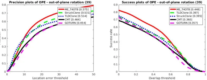
4.3 for a description of the elements of the figure. Best viewed in color. . 31 4.7 The increase in performance for out-of-plane rotation. . . 32 4.8 The decrease in performance for low resolution. . . 33
4.9 Relationship between the number of normal samples as a function of the Jaccard index. Higher Jaccard indexes present the additional
challenge that a smaller percentage of data can be used for training. . . . 37 4.10 Relationship between the number of anomalous samples as a
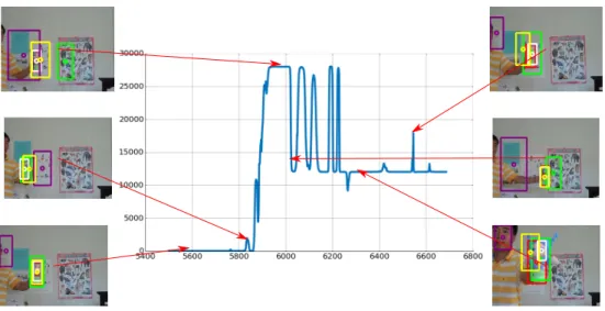
function of the Jaccard index. . . 37 4.11 Illustration of the results generated using the approach based on Eq.
4.5 for the sequenceDoll. The red, green, white and purple boxes correspond to the outputs of TLD, CMT, STRUCK and GOTURN respectively. The yellow box is the output of the fused approach. This method is capable of detecting outliers but struggles in complex scenarios where motion is highly non-linear and the Kalman filters covariance fails to capture that appropriately, as indicated by the frames in which there are lost trackers but the value
ofWΓ shown in the center graph is relatively low. . . 38 4.12 By using the proposed Mahalanobis distance method in [68], we
generate the area under the curve (AUC) for various values ofτ. We
see that this method particularly struggles with STRUCK and higherτ. . 39 4.13 ROC curves for the Mahalanobis distance method atτ =.3 on a test
set. We notice that the Mahalanobis distance particularly struggles
with STRUCK and performance is not consistent across all trackers. . . . 40 4.14 Outlier detection using a KNN classifier with 10 neighbors on
testing set.τ =.3. . . 41 4.15 Outlier detection using a SVM classifier on testing set. τ =.3. . . 41 4.16 Schematic representation of the implementation of the autoencoder. . . 43 4.17 Area under the curve for the trackers for various values ofτusing
the method described in Section 3.2 and shown in Fig. 4.16. We note that similarly to the Mahalanobis distance, higherτ pose a tougher
problem and performance is worse for smallτas well. . . 44 4.18 ROC curves for the autoencoder method atτ =.3 on a test set. . . 44 4.19 Area under the curve for the trackers for various values ofτusing
the method described in 3.2 and shown in Fig. 4.16. We note that
similarly to the Mahalanobis distance, higherτ pose a tougher problem. 46 4.20 ROC curves for the Autoencoder method atτ =.3 on a test set. . . 46
4.21 Schematic representation of the implementation of the variational
autoencoder framework. . . 47 4.22 Area under the curve for the trackers for various values ofτon the
test set using the method described in 3.2 and shown in 4.21. We
note that the standard Autoencoder is a better discriminator. . . 48 4.23 ROC curves for the Variational Autoencoder method atτ =.3 on a
test set. . . 49 4.24 Our proposed network. The input vector consists of the feature
vectors computed at two consecutive frames, f(m−1) and f(m−2). The dimensionality of each layer is shown below the layer. In particular,
the bottleneck layer has dimensionality L3=8. . . 50
4.27 Area under the curve for the trackers for various values ofτusing the method described in Section 4.3.3 and shown in Fig. 4.24. We note the Autoencoder is capable of more robustly detecting
anomalies for higherτ. . . 52 4.28 ROC curves for the Autoencoder method atτ =.3 on a test set. We
observe improvement in three of the trackers. The exception is GOTURN, for which the baseline approach in Figure.4.13 performs
better. . . 53 4.29 Illustration of the results generated using the proposed approach
based on autoencoders for the sequenceCar. See the caption of Fig. 4.30 for a description of the elements of the figure. We note that the reconstruction error from the autoencoder scales consistently with
the expected confidence of the trackers. . . 54 4.30 Illustration of the results generated using using the proposed
approach based on autoencoders. The images show snapshots of several frames in the sequenceDoll. The red, green, white and purple boxes correspond to the outputs of TLD, CMT, STRUCK and GOTURN respectively. The yellow box is the output of the fused approach. The graph in the center shows the values of the
reconstruction errors for the corresponding frames. We can see that higher reconstruction errors are associated with higher levels of anomaly. We also note that the reconstruction error decreases when
the trackers get closer to object of interest. . . 55 5.1 Final autoencoder model. . . 59
5.2 Histograms demonstrating reconstruction errors for allktrackers on the training set onτ =.3. The outliersFe(k)are blue and inliers F
(k)
l
are in green. Best viewed in color. . . 61 5.3 Histograms demonstrating reconstruction errors for allktrackers on
the test set onτ =.3. The outliersFe2(n) are blue and inliersFl2(n) are
in green. Best viewed in color. . . 62 5.4 ROC curves comparing the performance of thektrackers with
τ =.3. The left graph demonstrates performance on the training set F1and graph on the right corresponds to the test setF2. This ROC
is different in that each tracker has a dedicated network . . . 63 5.5 Precision recall curves comparing the performance of thentrackers
onτ =.3. The left graph demonstrates performance on the training
setF1and graph on the right corresponds to the test setF2. . . 64
5.6 Precision recall curves comparing the performance of thentrackers onτ =.3 using the Mahalanobis distance metric. The left graph demonstrates performance on the training setF1and graph on the
right corresponds to the test setF2. . . 65 5.7 Example of the probability distribution for the positive and negative
classes generated where green corresponds the positive class and
negative class is represented as blue. Best viewed in color. . . 67 5.8 Summary of our reconstruction error based scoring approach. Best
viewed in color. . . 70 5.9 Illustration of the performance of then=4 trackers and the
previous global estimate on theboltsequence. Refer to Fig. 4.3 for a
description of the various bounding box colors. Best viewed in color. . . 71 5.10 Reconstruction error$. Blue, green, grey and purple correspond to
TLD, CMT, STRUCK and GOTURN, respectively. Best viewed in color. . 72 5.11 Pkfor allktrackers TLD, CMT, STRUCK and GOTURN in blue,
green, grey and purple respectively. We can see that GOTURN has the highest amount of trust, but we also observe a drift up in value.
5.12 Pkwith the offset for allktrackers TLD, CMT, STRUCK and
GOTURN in blue, green, grey and purple respectively. We see the benefit provided by the offset by shifting GOTURN towards−1 which would imply that our algorithm completely trusts the tracker
for those frames. Best viewed in color. . . 74 5.13 Box and whisker plot showing the distribution of the tangent of the
likelihood tanh(κ∗(Pk−ψ))for variousτ of the ground truth for
allktrackers; TLD (top left), CMT (top right), Struck (bottom left) and GOTURN (bottom right). The red line represents the median for that specificτ value, the stars represent outliers in the data. The boxes correspond to the 1st and 4th quartile, the whiskers
correspond to 1.5 multiplied by the interquartile range. In general, for smallerτ, our method predicts the outlier and for higherτ it
correctly tends to predict that the object is an inlier. . . 75 5.14 Schematic representation of the implementation of the proposed
framework. Note how the Kalman filter blocks from Fig. 4.1 are
replaced by our autoencoders. Best viewed in color. . . 77 5.15 Scenario illustrating the case when only the two worst trackers in
the ensembles are correct, whereas the generally superior TLD and STRUCK are completely failing. This figure shows the benefit and practical significance of our algorithm. A design choice based on the best all-purpose tracker might not have represented the most
effective solution. See the caption of Fig. 5.16 for a description of the
elements of the figure. Best viewed in color. . . 78 5.16 Success shown when only GOTURN is correct. The red, green, white
and purple boxes correspond to the outputs of TLD, CMT, STRUCK and GOTURN respectively. The yellow box is the output of the
fused approach. Best viewed in color. . . 79 5.17 Robustness to failure from all but one of the trackers. We see that
STRUCK is correctly chosen to be trusted here. See the caption of Fig. 5.16 for a description of the elements of the figure. Best viewed
in color. . . 80 5.18 Robustness to the failure of multiple trackers. Here, we also observe
that the algorithm correctly chooses to trust TLD more. See the caption of Fig. 5.16 for a description of the elements of the figure.
5.19 Results of our Tracker (BAMAPDF) on OPE for OTB-50 compared to
the original implementation. . . 81 5.20 Results of our Tracker (BAMAPDF) on OPE for the Low Resolution
case, here we see the largest improvement relative to the initial
implementation. . . 82 5.21 Results of our Tracker (BAMAPDF) on occlusion, here the
improvement is the smallest, but small incremental improvement is seen. 83 6.1 Schematic representation of our proposed final goal. Best viewed in
CHAPTER 1 INTRODUCTION
With the current industrial, commercial and consumer market trends, it is evident that autonomous vehicles and semi-guided machines represent an active research area that is transitioning from theory to product. In this context, the majority of these systems is supported by vision-based tracking algorithms. Extensive and ambitious projects such as Amazon’s drone delivery service [34], Uber [7], Tesla’s self driving cars [19] and the first woman robot Sophia [22], exemplify just how rapidly robotics enter into our everyday lives. Unmanned Aerial Vehicles or UAVs are especially advantageous due to their relatively cheap cost and aerial nature. However, all of these products are not new, but rather they are the sum of hierarchical building blocks and incremental progress. Recent advancements in autonomous UAVs can be attributed to a few factors, including stronger and more compact computing, image processing and computer vision, machine learning and powerful sensors. Rather than being isolated
developments, these advancements have all been intrinsically linked by growth in processing power for the onboard computer of these systems.
In this field, the problem of object following and its sub-problem of
tracking are of great relevance. In fact, many state-of-the-art robotics applications require powerful and robust trackers [66, 28]. In tracking, there are many
different approaches that have been proposed. Visual, global positioning systems (GPS) and infrared remain commonly used [5]. Visual tracking began first with template matching, a simple algorithm that has many limitations such as the simple model that does not update and the simple representation of the target. Afterwards, there was a transition to more sophisticated solutions such as
early machine learning approaches based on algorithms such as support vector machines (SVM) [25], ensembling [58] and K-nearest neighbors (KNN) [35] were proposed. Finally, the past 12 years have seen the rise of deep neural network based approaches which have been revolutionary in the field of computer vision which includes the seminal Alexnet [43]. Previous tasks such as image
classification have seen great strides, and helped introduce new tracking
approaches. While state-of-art deep neural network (DNN) based trackers such as MDNet [61], SANet [20] and DCPF [31] effectively outclass most of the previous approaches, unfortunately, they remain too slow for real-time
application. With new research in skip connections [26], attention models [81], dilated/atrous convolutions [80], reinforcement learning [49] and capsule
networks [72], it remains probable that improvements are on the horizon. While all of the approaches provide significant improvements, we address the
fundamental issue of robustness by proposing an algorithm that can fuse information from various single object vision trackers to provide robustness at the cost of computational complexity. Our definition of robustness includes both generality, such that the network can operate well in many different scenarios and a tolerance to faults. One of the fundamental advantages of the deep learning revolution has been to introduce deep networks, that with sufficient data, can construct regression models that model complex unknown mathematical behaviors. Our aim is to leverage this tool to learn the operation of any type of tracker to model normal operation. Once our network can model normal operation, we use this information to act as a weight in a fusion step.
Because robustness is so important in critical systems, it has received a lot of attention. In autonomous vehicles, any sort of error can be extremely costly, and therefore many systems include redundancies in order to improve
fusion. Sensor fusion rose to prominence with the invention of the linear Kalman filter (KF) in the 1960s [10]. However, the linear KF has limitations including the Markov assumption [10] and it assumes a linear motion. Subsequent innovations such as the Extended and Unscented Kalman filter [10] have tried to address this issue with varying levels of success. Further improvements that sought to
incorporate prior information introduced other Bayesian methods such as Particle filters [17]. As in tracking, machine learning also became prominent in sensor fusion and in combining classifiers. SVMs [48], Naive Bayes [45], Majority
voting [45] and Adaboost [1] have been powerful techniques that are well known and also well understood. With the deep learning revolution, deep neural
networks have been used to fuse results from different sensors [13], learn values for a deep Kalman filter [40] and fuse different types of information in a siamese network [4]. We build upon the work of Echeverri et al. [18] which already uses Kalman filters and simpler machine learning techniques by applying deep networks to learn powerful representations of the intrinsic characteristics of properly functioning trackers. We integrate deep Bayesian autoencoders into this framework to improve performance.
To train our networks, we first collect data on the OTB-100 dataset [84]. This is a dataset that contains 100 distinct images sequences with a moving target. For each of these videos, algorithms are given the initial location of the object. After the trackers run through these video sequences, a MATLAB script evaluates all trackers’ performance on these videos. By running our tracker ensemble on this dataset we can collect the results of various trackers. Because this dataset contains the ground truth, the results can be split into various partitions. We look at different subsets to find representative data that we use to train networks that recognize distinct anomalies. We formulate the score as a maximum likelihood probability [45] similar to a naive Bayes approach to penalize anomalies. Later,
we add this feature to the ensemble and run the sensor fusion algorithm on the benchmark. After evaluating this new algorithm on the benchmark, we look at its performance on a test and training set of videos.
Our final goal is to deploy the algorithm on a UAV drone and use the Matrice 100, DJI SDK [71] and add PID controls based in part on the work in [66] to have the drone follow a target. We would qualitatively compare performance to available commercial applications; namely the DJI Mavic. To compare, we would first look at the previous AR-parrot version described in [18] to determine whether our new solution provided any significant improvements. Our future tests would be to perform a quantitative analysis by examining the number of frames the drone can successfully follow a target for 3 different
scenarios/environments. This includes outdoors, indoors and stationary. Here we could measure success by how many consequent frames the drone can follow a target and compare that to its competitor.
1.1 Contributions
The contribution of this thesis is the creation of a Bayesian Autoencoder Maximum A Posteriori Data Fusion framework (BAMAPDF). The purpose of this research is to improve upon the Hierarchical Bayesian Data Fusion (HABDF) algorithm developed in [18]. More specifically, the contributions are as follows:
1. Acquire training data from different trackers, partitioning and properly scaling data.
2. Explore different machine learning approaches to detect anomalies. 3. Integrate the trained models into the tracker ensemble to improve
robustness.
The thesis is organized as follows. Chapter 2 introduces ideas that
that this thesis builds upon. In Chapter 4, we evaluate the HABDF
framework,present our data partitioning method and evaluate various machine learning based anomaly detection methods. In Chapter 5, we explain how we used the outlier detection results to modify the initial sensor fusion approach. In our conclusion, we summarize our work, and discuss future research on how to integrate the proposed method on a following UAV.
CHAPTER 2 LITERATURE REVIEW
This chapter is structured into four sections. The first section discusses related work on vision-based target tracking. Secondly, we introduce the
proposed data fusion approach as the main contribution. Next, we look at related work on anomaly detection and introduce our choice of autoencoders. Lastly, we look at work related to UAVs and object following as a real-life application to our modified algorithm.
2.1 Tracking
Given an initial video frame and a bounding box that delimits an object of interest in that frame, the purpose of a single-target tracking algorithm is to follow this object through subsequent frames without being told the new
bounding box that encompasses the object. This is relevant in many applications such as surveillance and autonomous driving where one needs to keep track of a single object over consecutive frames. While the problem sounds simple to a human, it is difficult for a machine due to the uncertain nature of this problem. Changes in lighting are trivial to us, but to a machine this change in the
mathematical representation of the whole image is difficult to handle without a mathematical representation of this change and the conditions of this change. Due to the very open-ended and multifaceted nature of this problem, a myriad of different trackers has been developed.
Trackers such as TLD [35], for example, use a nearest neighbor based approach to address the issue of tracking an object between frames.
State-of-the-art trackers such as GOTURN [27], use deep convolutional neural networks to track objects in a search space. Due to their inherent design
characteristics, the performance of these trackers differ with respect to issues such as occlusion, illumination, motion, deformation, blur and rotation. As such, different trackers have been found to perform better depending on the scenario. With this in mind, while some trackers show overall better performance in standardized datasets, there are instances in which these trackers are
outperformed by less sophisticated methods due to the fact that they do not handle a particular situation well. As it stands now, the tracking problem is still a largely open research topic.
2.1.1 Sensor Fusion
To generate more robust predictions, typically a common approach is to combine results from multiple sources. In fact, certain trackers are just
combinations of a large amount of weaker trackers that work together [88]. Sensor fusion has been an intense area of research in controls and electrical
engineering. The idea of adaptive fusion began in the 1960s with the introduction of the Kalman filter (KF). In the 1990s, the approach became more widespread with the development of variations of the initial algorithms based, for example, on the extended KF or the unscented KF [76]. Particle filters (PF) [23] and fuzzy logic [8] have also recently gained popularity. Some preliminary work has even been done on combining deep neural networks and Kalman Filters [40]. Each of these methods assumes some sort of prior knowledge about the trajectory of what is being tracked. For single-object-tracking, this is generally a valid assumption given the relatively locally linear nature of the motion of most objects when observed at reasonable frame rates. Our work is most similar to the work done by Bailer [3] and Biresaw [6], which use a hierarchical state fusion interpretation. However, we use a different data fusion approach than Biresaw, and our
Bailer. Additionally, similar Bayesian frameworks were proposed by Yang [86] to perform multimodal tracking for healthcare applications with the use of different weighting schemes. One of the most common modern approaches to data fusion is the use of machine learning. These methods are powerful but are challenging to implement practically due to their reliance on large amounts of training data. The approach presented in this paper mitigates these issues by using an adaptive Bayesian model that adapts its behavior based on the performance of the trackers and by using a semi supervised approach that reduces the amount of training data needed. A hierarchical Bayesian data fusion approach requires only that the user provides weights to the trackers as a tuning parameter and a motion model which can be assumed to be linear.
2.2 Anomaly Detection
On the topic of anomaly detection, a myriad of methods have been proposed. Recently, the development of machine learning has allowed for complex rules to be derived to quantify errors. Common approaches include SVMs [64], Decision Trees [78], Naive Bayes [2] and Adaboost [29]. However, all of these methods are supervised and require labeled positive and negative data. While attempts have been made for unsupervised approaches such as the One-class SVM [79], results have been mixed. Other unsupervised approaches such as K-means have also been proposed, but unfortunately, this algorithm generates many classes and suffers in performance with large-dimensional data. Recently, deep learning has made tremendous strides in dealing with the issue of high dimensional data. In particular, autoencoders have been used as a way to reduce the dimensionality of data in a manner similar to PCA [69] by learning non-linear transformations.
Data fusion for object tracking has been explored in great detail in works such as [6, 11, 3]. The method of using confidence scores with a majority vote for data fusion was first proposed in Echeverri et al. [18] and later evaluated in this thesis. That method, referred to as Hierarchical Adaptive Bayesian Data Fusion (HABDF), has the advantage of being computationally inexpensive. However, one weakness of that approach is its susceptibility to anomalous tracker outputs. In particular, this is because the confidence score uses a Mahalanobis score to determine whether the tracker is an outlier based on [67]. This is problematic because the underlying assumption is that object motion is linear and noise is Gaussian. For tracking, this assumption does not always hold due to the non-linear nature of object motion in the wild. Therefore, the ability to handle situations where this assumption fails is important to improving performance.
Detecting outliers in a tracker is difficult because if a tracker knew when it was wrong, it would be able to self-correct preemptively and not make the
mistake in the first place. A robust outlier detection mechanism is of particular interest for vision-based trackers. Penalizing anomalies is commonly used in tracker ensembles and sensor fusion. Normally, when the algorithm decides that a tracker is lost, it might discard the results or apply a smaller amount to that trackers result so its effect will be trivial or ignored. Better anomaly detection in each of these approaches would naturally lead to better results. One successful approach to determine that a tracker is lost was proposed in [83]. Unfortunately, that method is only applicable to trackers that employ correlation filters because it is dependent on the distribution of the correlation map generated by the network.
Autoencoders have shown great potential as a tool for anomaly detection [90, 50, 79]. However, to our knowledge no work has explored their use as a weighing mechanism for tracker ensembles. The methods proposed in [33, 38] are perhaps the closest to our work, albeit they were applied to the different
problems of monitoring wind turbines and electrocardiograms. Our method builds on the works proposed in [33, 38] by building feature vectors consisting of several estimates of the positions and velocities of the target, which are generated by Kalman filters that use the ouputs of the individual trackers as observations. In addition, these feature vectors are constructed using consecutive image frames, thereby further incorporating the temporal relationships between the outputs generated by trackers.
2.3 Unmanned Aerial Vehicles
Unmanned UAVs or drones have recently captured the public’s attention. Follow-me UAVs are an especially interesting area of research due to their
application in the film industry. These are UAVs that receive a specified target and then attempt to follow the target with the camera focused on that target and controlled so that the target is in the center of the image. Rather than having someone control a camera to follow a scene an automated drone would decrease costs and lead to more freedom for artistic expression. Most higher end UAV platforms have some sort of onboard program to accomplish this task. In general, this is usually accomplished in one of two ways; using GPS [16]/Ground Station Control [65] or using recognition/tracking [66]. Using a ground station requires that the object of interest has some of device that allows the UAV to triangulate to the objects location. However, this incurs the issue that the device is intrusive. For very close following, the GPS is unreliable unless a very expensive option is chosen [54]. Using a ground station that relies on other signal types such as WiFi is possible but leads to issues associated with latency. An image based following approach has been accepted as the preferred method when dealing with smaller distances [54]. In particular, the work by Pestana [66] was instrumental in
addition to attempting to keep the target at the center of the image using its centroid position (r,s), the UAV also used the target’s relative scale variations, based ontandu, to keep a constant distance from the target. Essentially, the drone would follow a target within a fixed distance, attempting to maneuver so that the target remains in the center of the video frame.
Our goal in this thesis is to improving our tracking performance by adding robustness via a more powerful fusion approach. To do this, we frame our fusion trust mechanism as an anomaly detection/anomaly score problem.
CHAPTER 3 BACKGROUND
Here, we introduce Hierarchical Bayesian Data Fusion (HABDF), the algorithm this thesis seeks to improve. We also evaluate this method and set it as reference to our approach. Next, we explain the theoretical foundations of
autoencoders, which act as our main tool in improving HABDF. 3.1 Hierarchical Bayesian Data Fusion for Target Tracking
HABDF is a variation of the mixture of experts framework [87]. The main difference is that the gate is substituted with a Bayesian approach. Each separate trackersjacts as an “expert” asynchronously when it is run through a Kalman
filter. The motion and observation models are given by
x(t) = Ax(t−1) +w(t) (3.1)
y(t) = Cx(t) +v(t), (3.2)
wherexis the state vector andyis the observation vector. Eq. 3.1 represents the system dynamics withArepresenting the transition matrix,Bbeing the control matrix andwmodeling process noise. In Eq. 3.2,Cis the observation matrix, and
vis the measurement noise. Both of the noises are assumed to be white and Gaussian with variancesRwwandRvv. HABDF uses two sources of information
to penalize detectors and to vote on a global output. The first mechanism through which the framework assigns weights to each of the detectors is based on the Mahalanobis distances (MD) [53] of the observations, whereµis equal to prediction, andΣis the covariance.
Ω(y) =
q
As shown by Pinho [67] the MD can be approximated by Ω(y) = N
∑
i=1 (yi−µi)2 Σii ! , (3.4)whereyiandµiare the elements ofyandµandΣii are the diagonal elements of
the innovation covariance matrixΣ.
Rather than using the MD values directly as weights in our framework, in order to soften transitions as the performance of the individual trackers
fluctuates, a sigmoid function is employed
wM = 1
1+e(−Ω(y)+ξ), (3.5)
whereξis a value chosen based on theχ2number of degrees of freedom of the system and the desired confidence level. This step takes advantage of the
Bayesian framework but rather than using those statistics to correct the tracker as done in [51, 46], here they are applied as weights in a voting scheme. This
generates a score that penalizes trackers for being far away to the other nearest tracker.
The other mechanism involved in the assignment of weights to the outputs of the individual trackers is the majority voting scheme based on the pairwise Euclidean distances between the various trackers. Letxiandxjrepresent the state
vectors corresponding to two different trackers. Let the Euclidean distance betweenxiand xj be
di,j =||xi−xj||. (3.6)
Then,mindrepresents the smallest distance between trackeriand all of the other
trackers in the framework.
mind= min j=1,2,...,n
j6=i
Again a softening mechanism is applied to avoid abrupt changes in the tracker operation. In this case, the method chosen was a hyperbolic tangent function
wd=ω0+ω(1+tanh(mind−λ)), (3.8)
whereω0is the minimum value andλrepresents the minimum required for the penalization to take place.
The filtered outputs of all the trackers, bounding boxesxj, are provided as
inputs to another KF. This acts as the fusion center. The fusion center adapts itself to changes in the performance of individual trackers after each new measurement is collected by updating its measurement noise covariance according to
Rσσ(wd,wM) =Γwd+∆wM, (3.9)
whereΓ=diag(γ1,γ2,· · · ,γn),∆ =diag(δ1,δ2,· · · ,δn), anddiag(.)represents a
diagonal matrix whose elements are the function parameters.γiandδi are set to 1
if there is no a priori knowledge of the system, but they can be adjusted individually if there is prior information about expected tracker performance. That is, the majority voting weightwdand the MD weightwMare used by the
global tracker to updateRσσ, which is then used in the global correction stage of
the Kalman filter to generate the fused bounding boxxf. Eq. 3.9 allows the
Kalman filter to trust less in measurements that have lower weights. The Kalman filter for the fusion center is essentially identical to those applied to the individual trackers (Eqs. 3.1, 3.2) but the observation matrixCreflects the fact that the
observations are given by the outputs of thentrackers. Algorithm 1 summarizes the HABDF algorithm.
Algorithm 1HABDF
Input: Set ofntrackerssj ∈ S, initial bounding boxx0, setV of images
Output: Bounding boxsf representing the fused output 1: Initialize all trackerssjwith x0.
2: Initialize Kalman filter for each algorithm implementationsj 3: Initialize Kalman filter for fused data model
4: whileVhas new imagesdo
5: Load new image
6: forEach trackersj ∈ Sdo
7: Generate bounding boxxjfor each trackersj 8: Apply Kalman filter (Eq. 3.1,3.2) toxj
9: Compute Mahalanobis Distance weightwM 10: end for
11: Wait for all trackerssj
12: Apply majority voting to findwd 13: Calculate Rσσaccording to Eq. (3.9)
14: Apply Kalman filter (Eq. 3.1,3.2) using Rσσ as the observation covariance
to generate
the global estimate xf 15: end while
3.1.1 Additions to HABDF
In this thesis, we added the tracker GOTURN [27] to the ensemble. This tracker was considered a state-of-the-art real-time neural network based tracker at the time we started. To work as a tracker on a video benchmark, modifications had to be made. Because the original algorithm used asynchronous calculations for maximum speed, so that calculation speed depended only on the fastest tracker, the algorithm could skip frames. To rectify this, the algorithm was modified to be synchronized to the slowest tracker. Although this approach penalized the algorithm’s speed, it could still operate in real-time. Additionally, accuracy and robustness was improved. By incorporating additional locks, concurrency issues in the threading were addressed.
3.2 Autoencoder
A important current research topic is the problem of outlier detection. Outlier detection, fault detection, anomaly detection are used interchangeably and refer to the concept of detecting when operation stops being “normal”. In power transmission this would be when current through a line drastically
increases, commonly known as a three phase fault. When this is the case, we can see that this is happening with sensors and normally a relay is triggered to stop the current from flowing and damaging the transmission line. Other faults can occur in different types of systems from different application domains including raw vibration signals [89], turbines [33], altitude estimation [24] and big data [52]. This concept has many applications in fields of research including: tracking, big data, object detection and machine learning. Additionally, it is also an important standalone topic in areas such as aviation [32]. In object tracking, methods that rely on Bayesian estimation are not robust to anomalous data, especially since these methods use prior data to make an estimate. If a previous estimate is poor it can throw off a tracker, which will remain lost and hurt the final estimate. To improve outlier detection, several methods have been proposed [57]. One of the most promising solutions seems to be the machine learning approach due to the unique power of machine learning to learn non-linear abstractions [77]. One route of machine learning that seems to be promising is the use of autoencoders. Autoencoders are neural networks that model the target function input = output, and by doing so they learn a model for the latent space of expected data [42].
For any input example vector or matrixx∈ Rn, we can generate a hidden
representationh(x)∈ Rm by using a non-linear activation function applied to every component. We chose to use the hyperbolic tangent because it provided the best results experimentally, but many other options are available. WithW as the
weight matrix, andιrepresenting the bias vector we can formulate the encoder:
h(x) = f(W1x+ι1), (3.10)
where the activation function f(z)is equal to the hyperbolic tangent,
f(z) =tanh(z), (3.11)
The decoder of the autoencoder then maps the hidden representation to the reconstruction ˜x∈ Rn:
˜
x = f(W2x+ι2), (3.12)
Normally, multiple layers are stacked in the encoder and decoder in a descending manner to force the network to learn a latent representation of our data. Training the autoencoder is then done to find the parameters that minimize the mean squared error. With an input set of examplesΞwhich can be defined as :
Φ(θ) =
∑
x∈Ξ
kx−x˜k2. (3.13)
Gaussian noise is usually added during training to the input to improve performance the networks performance by minimizing overfitting. Noise is added by corrupting the inputxinto corrupted input ´x|x ∼N(x,σ2I).
This added benefit assists the network in learning a better latent representation[56]. Stochastic gradient descent is generally used due to find weights that minimize the mean squared error through backpropogation, but there are other options available such as Adam or RMSprop. In our work, we generally used RMSprop [70].
By taking advantage of the inherent ability of these neural networks to learn what governs “normal operation”, it is then possible to extrapolate what is “unexpected” data. There are many methods that take advantage of this model and most of them use either the dimensionality reduction or the reconstruction
error to detect outliers [50]. We use the reconstruction error as a threshold which can defined be defined as
$=kx−x˜k2 (3.14)
3.2.1 Variational Autoencoder
To better model the probability model associated with many different types of datasets, further advances in machine learning have led to the creation of variational autoencoders [37]. The variational autoencoder uses hidden layers to learn latent representations in a manner similar to regular autoencoders.
However, the difference is that the bottleneck layer encodes to a Gaussian probability density,
qθ(z|x) ∼N(ηz,ζz), (3.15)
Whereηz andζzare the mean and standard deviation of the distribution,
respectively. Our encoded value is now z. To decode z the decoder outputs the parameter associated with each probability distribution of the data,
pφ(x|z) ∼N(ηz,ζz). (3.16)
We can measure the loss function as a function of the information lost associated with the decoder as the sum of the reconstruction error of the representation or the mean squared error 3.13 and the Kullback-Leibler divergence between the encoder described in equation. 3.15 and a Gaussian distribution (normally mean zero and variance one).
Φi =−Ez∼qφ(z|xi)[logpφ(xi|z)] +KL(qθ(z|xi)||N(0, 1)), (3.17)
Where the Kullback-Leibler divergence is defined as
E logqθ(z|x) ∼N(ηz,ζz) pφ(x|z) . (3.18)
The Kullback-Leibler divergence attempts to force the latent distribution by penalizing the bottleneck distribution to fit the normal distribution.
−Ez∼qφ(z|xi)[logpφ(xi|z)]generally is approximated as the mean-squared error.
This is particularly relevant to our application because we predict that the variational autoencoder has the smallest possible reconstruction error for the good data, and that mapping occurs in such a manner that prevents overfitting by encouraging dispersion of the latent representation.
3.2.2 Convolutional Autoencoders
To assist our network in learning the temporal dependencies we also explored using 1D convolution layers in a manner similar to Wavenet [80]. This changes our neurons to become the convolution of the input and weight matrix from the previous layer. As expressed in [38], we define our network activationsα for layerlfor allυneurons as
α(fl) =
Nl−1
∑
i=l
σ(Wilυ−1∗ fil−1) +ιlυ, (3.19)
where “∗” is the 1-dimensional convolution operator and σ(·)is the non-linear hyperbolic tangent activation function. An important consequence is that because of the convolution operator, our hidden layers are 2D. The last layer of a
convolutional autoencoders is usually a flatten layer that brings the shape back to 1D.
In a similar manner, a 2D autoencoder can also be used to convolve 2D representations of data by modifying 3.19 to use higher dimensional tensors. Most image based applications use convolutional neural networks to achieve state-of-the-art results [15].
3.2.3 Apples and Oranges Example
To better illustrate how autoencoders can be used to detect anomalies we present the example of apples and oranges based in part on the work in
Imagenet [44]. Imagenet is a dataset of over a million photos of different classes. One of the most well known neural networks used to classify different images and accomplish this task is VGG [73]. We base our encoder and decoder
architecture heavily on the first 4 layers of VGG with one low-dimensional layer in the middle. As seen in the work by Dias [15], the network is capable of
capturing representations of a complex class into a latent space. By taking advantage of Imagenet, we first acquired 100 images of the apple class and 100 images of the orange class. Next, to give our network more training examples we used the method detailed in [44] to generate more data because Imagenet does have many photos only a small minority are apples. Afterwards, we built a neural network based heavily on the Imagenet network architecture. At the bottleneck layer, rather than feeding the data into a dense layer, we used
convolutions as described in Eq. 3.19, to upsample so that our output is the same size as our input. Using the mean squared error, Eq. 3.14, as the loss function, and using the apple photos as the input and output, we were able to learn a function to model the apples by running a stochastic gradient algorithm to minimize the loss. After running enough iterations so that the loss function begins to converge, the model can be deployed to run predictions. In Fig. 3.1, we see the result of passing various images of apples through the network. Even though the output image is not a perfect reconstruction, we see that the result still looks very similar to an apple. However, we also observe that the orange fruit reconstructions do not look like oranges, in fact they are quite apple-like. Because the network is trained only to reconstruct apples, the oranges have features that
Figure 3.1: Reconstruction of apples and oranges. The top image is the original picture, the bottom is the reconstruction passed through the autoencoder. Best viewed in color.
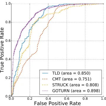
are apple-like. The above result is confirmed in Fig. 3.2, where we see that on average the standard Euclidean distance from Eq. 3.14 between the
reconstructions for the apples is smaller than that for the oranges. We conclude that we can use autoencoders to learn a meaningful
representation of what “apple” means. By taking advantage of this, we can use autoencoders to differentiate between apples and a class it has never seen; “oranges”. Because the class is balanced we generate an ROC curve [9], that compares the different thresholds and their associated false positive and true positive rates. These curves tell how accurately the classifier can predict outliers and how many false alarms it will generate for a threshold. By using the
reconstruction error as a metric we can see how well it is able to discriminate between apples and oranges in Fig. 3.2, right hand side.
If we were to modify our network by substituting the bottleneck based on Eq. 3.17, we can train a new network keeping everything else relatively constant.
0 2 0 4 0 6 0 8 0 1 0 0 1 2 0 1 4 0 1 6 0 7 .5 1 0 .0 1 2 .5 1 5 .0 1 7 .5 2 0 .0 2 2 .5 2 5 .0 MSE Frame number R econstr uction er ror 0.0 0.2 0.4 0.6 0.8 1.0 False Positive Rate
0.0 0.2 0.4 0.6 0.8 1.0 Tr ue Po si ti ve R at e Training Data AUC (area = 0.70)
Figure 3.2: The graph on the top shows the mean squared error values of apples and oranges. The first 80 values correspond to the reconstruction error for apples and values 80−160 correspond to the reconstruction error for the oranges. On the bottom we show the associated ROC curve.
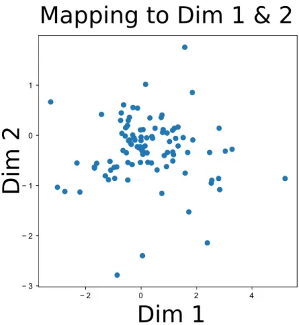
The primary benefit of this is that now the feature space of the data is dispersed according to a multidimensional Gaussian (see Fig. 3.3) where the points
represent apples in two dimensions of the feature space. If we sample from a random multidimensional Gaussian with the same shape as the bottleneck layer and pass those values through the decoding stage we can see what the network
−2 0 2 4 −3 −2 −1 0 1
Dim 1
Dim 2
Mapping to Dim 1 & 2
Figure 3.3: Dispersement of values for Variational autoencoder in the bottleneck layer. The dots represent the mapping of various apple images. We observe that the latent mapping looks like a Gaussian distribution.
thinks an “apple” looks like in Figure 3.4.
While the rest of the thesis does not deal with apples, this example illustrates the fundamental idea of how autoencoders can be used to detect anomalies as well as their benefit. Even though classifying between apples and oranges is a relatively easy task (even for a computer), a large benefit of this approach is that the network can “learn” to approximate what it means to be an “apple”. An additional benefit is that the network is not only capable of
discriminating between apples and oranges but also between apples and other different images. In our work, “apples” represent the idealized data of what we expect our trackers to operate under normal conditions. The “oranges” are the
Figure 3.4: Variational autoencoder generated “apples”. Best viewed in color.
CHAPTER 4
DATA GENERATION AND AUTOENCODER DESIGN
In this chapter, we first explore HABDF, the tracker ensemble that this work builds upon. We look at the ensemble’s performance and evaluate it using the OTB-50 benchmark. We briefly describe some of the issues with HABDF and what motivated our exploration of the alternatives to the Mahalanobis Distance weighing. Next, we explain how this ensemble can be used to generate training data. Here we also explain how this data can be transformed into datasets that allow us the test the anomaly detection performance of different algorithms. Finally, we explore and compare different methods, arriving at our proposed method of using Autoencoders.
4.1 HABDF Evaluation
First, we evaluate the reference method (HABDF) to determine its strengths and weaknesses. To do this, we take advantage of publicly available benchmarks.
4.1.1 Visual Tracking Benchmarks
To measure that the output of our data fusion method is working better than the trackers that comprise it, it is necessary to test the results on a
benchmark. The OTB-50 benchmark is one of the most common tools used to evaluate various performance scores. Originally introduced in [85], the OTB-50 benchmark has 50 specific data sequences that it uses to provide different measurements of performance on various attributes. The most general of these measurements is the success, which measures how well the tracker can track the object throughout all of the image sequences. The OTB benchmark makes it
possible to quantitatively evaluate the results generated by the tracker. Other publicly available visual tracking benchmark datasets include VOT [41] and ALOV [75]. We chose OTB-50 due to its simple integration and popularity. We would also like to note here that OTB-50 is part of OTB-100. OTB-50 selects 50 of the sequences from OTB-100, and changes these sequences periodically. This is so that there exists a smaller subset for faster testing.
4.1.2 HABDF OTB-50 Results
Our initial contribution was to evaluate the method proposed in [18] on a visual tracking benchmark. To do so, first we added the changes described in Section 3.1.1. The block diagram of our implementation is show in Fig. 4.1. We initially carried out separate evaluations of the four trackers that comprise our implementation of the proposed framework on the OTB-50 dataset. For
STRUCK1and TLD2our results were 3% worse than the results reported
in [35, 25], this is likely due to the changing sequences in the OTB-50 evaluation. For CMT and GOTURN, to the best of our knowledge, OTB-50 results are not publicly available so those had to be generated3. We then evaluated our approach on the same dataset with these same four trackers as part of our ensemble. We adjusted the values ofωproportionally to the success rate of each of the trackers on the OTB-50 dataset. The method showed a 5.5% increase in success relative to the best tracker in the ensemble and a 2.6% increase in precision. Since our
method focuses on improving the overall robustness of the trackers, we expected the larger increase in success rate. The improvement in precision demonstrates that this method is not penalized by “imprecise” trackers such as CMT.
1the results were obtained using source code available at https://github.com/samhare/struck
2the results were obtained using source code available at https://github.com/klahaag/CFtld
3the results for CMT and GOTURN [27] were obtained using source code available at
https://github.com/gnebehay/CMT and https://github.com/davheld/GOTURN respectively. We applied these methods “as shipped”.
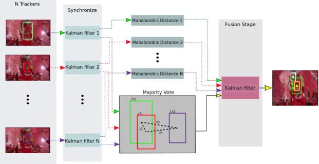
Kalman lter 1 Kalman lter 2 Kalman lter N Mahalanobis Distance 2 Mahalanobis Distance 1 Mahalanobis Distance N Fusion Stage Synchronize N Trackers d2 d 1 d3 D3 D2 D1 Majority Vote
Figure 4.1: Schematic representation of the implementation of the baseline framework. Best viewed in color.
Figure 4.2: Results of our Tracker HABDF (referred to as ME T4) on OPE for OTB-50
Our results in Figure 4.2 illustrate the performance of the proposed approach.We see that our method shows improvement in both precision and success. In particular, we see that our method has higher for location error
rate for overlap thresholds less than .6, this implies that our algorithm has more frames where this some overlap with the ground truth. Our ensemble leverages the individual strengths of each tracker to obtain higher levels of robustness throughout the various datasets. Even the best tracker in our ensemble
performed poorly in certain scenarios, and despite providing the largest influence on the input, the other trackers helped improve performance overall.
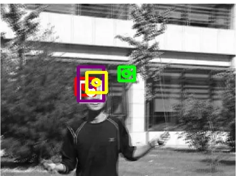
Our ensemble is robust to failures from the lower ranked trackers such as GOTURN or CMT, and the failures of these trackers did not affect the overall performance when they occurred individually as seen in Figures 4.3 and 4.4. In the Figures our tracker is denoted by the yellow bounding box, and the color scheme for the other trackers is red/blue for TLD (blue when it is lost since TLD can make that determination), purple for GOTURN, green for CMT and white for Struck.
Figures 4.5 and 4.6 illustrate that our tracker is also robust to failures generated by the stronger trackers in the ensemble such as TLD or Struck.
Figure 4.3: Robustness to failure from GOTURN. The red, green, white and purple boxes correspond to the outputs of TLD, CMT, STRUCK and GOTURN respectively. The yellow box is the output of the fused approach. Best viewed in color.
Figure 4.4: Robustness to failure due to CMT. See the caption of Fig. 4.3 for a description of the elements of the figure. Best viewed in color.
A simple majority voting approach would have allowed poorly
performing trackers to degrade the overall results. Our method mitigates this issue by assigning weights based on the Mahalanobis distances of the
measurements generated by each tracker, and also by incorporating previous knowledge about the performance of the individual trackers. In Figures 4.3 and 4.4, it can be observed that these anomalous measurements have a minimal effect on the overall tracking result. This is seen by the yellow fused result, that chooses to follow the other trackers rather than the anomalous one. In the first subfigure, GOTURN’s distance from the other trackers assigns the tracker a high weight due to Eq. 3.8. Hence, GOTURN has a minimal effect on the final estimate and
continues to do so due to the motion model associated with the resultant tracker.
Figure 4.5: Robustness to failure from the strongest tracker in the ensemble. See the caption of Fig. 4.3 for a description of the elements of the figure. Best viewed in color.
Figure 4.6: Robustness to the failure of multiple trackers. See the caption of Fig. 4.3 for a description of the elements of the figure. Best viewed in color.
In Figure 4.5, the best tracker in the ensemble, STRUCK, has failed. Because our weighing mechanism is not just a weighted voting scheme, our tracker is able to disregard the measurements from Struck. In the second figure, we see that two trackers are lost, but our ensemble is still able to perform very well. By taking advantage of the proximity between Struck and GOTURN as dictated by Eq. 3.8 these trackers have a much higher influence on the output. CMT and TLD, on the other hand, are far from any other tracker, accrue a higher penalty and do not significantly influence the output. It is also important to note that because of the weights applied using the Mahalanobis distance, the fusion approach penalizes erratic performance from trackers. The weights generated by the Mahalanobis distance allow the framework to smooth out the estimate and engender a more steady and more robust output. Besides positively impacting success and precision, the method also significantly increased the score where all the trackers had a similar score for the specific metric. This benefit is especially
obvious for the OPE of out-of-plane rotations. Despite the significant
improvement in most scenarios, in the rare situations where performance was drastically different among trackers, a decrease in performance was observed relative to the best tracker in the ensemble. When multiple trackers are
significantly worse than the best trackers, the performance may decrease. This is especially obvious for the case of low resolution images in which GOTURN and CMT perform very poorly and hence degrade the overall performance.
We present the complete results of our tracker relative to demonstrate that the fusion technique clearly increases robustness. Unfortunately, this increase in robustness means that sometimes the individual strengths of a tracker is lost. In particular, we point the motion blur and low resolution scenarios in Table 4.1.
As Table 4.1 indicates, our approach improves the performance in 8 of the 12 scenarios including; illumination, out-of-plane rotation, scale variation,
occlusion, deformation, in-plane rotation and background clutter. In the cases where the performance decreases, it is important to note the large discrepancy between the best tracker and the other trackers in the ensemble. Because the method uses the confidence generated by the Kalman filter, when multiple
Figure 4.8: The decrease in performance for low resolution.
trackers show poor performance, our results can be negatively affected. The improvement is most obvious and prominent when the trackers show similar performances. This problem can be mitigated by either refraining from using trackers that perform very poorly under certain scenarios or by adjusting its prior weight according to its worst-case performance.
4.1.3 HABDF Issues
A Bayesian data fusion approach was applied to the problem of
vision-based target tracking and showed promising results in the OTB-50 dataset. Significant increases in robustness were observed despite the weaknesses of certain trackers. The method provides an adaptive framework that uses both the local statistics generated by each tracker as well as a weighted majority voting mechanism to determine the target bounding box at each frame. Pretraining is not required, and the method is robust in practical scenarios due to its ability to integrate multiple sources of information.
One simple way to extend this work would be to consider the problem of outlier detection. If it is known with high probability that a tracker is lost, it can
Table 4.1: Summary of results on OPE Scenario Best Tracker Best Tracker Score (Precision /Success) Worst Tracker Worst Tracker Score (Precision /Success) Fusion Score (Precision /Success) Percent Change Relative to Best Tracker
Total Struck .581/.440 GOTURN .436/.337 .596/.464 +2.581% /
+5.454%
illumination Struck .581/.413 GOTURN .347/.291 .524/.427 +1.158% /
+3.389% out-of -plane ro-tation Struck /TLD .531/.397 GOTURN .454/.357 .575/.448 +8.286% / +12.846% scale variation Struck .562/.386 CMT .435/.327 .574/.432 +2.135% / +11.917% occlusion Struck/TLD .521/.408 CMT /GOTURN .404/.311 .548/.431 +5.182% / +5.637% deformation Struck .516/.414 CMT .373/.301 .568/.450 +10.078% / +8.696% motion blur Struck .487/.406 GOTURN .300/.254 .450/.366 8.222% / -10.929% fast motion Struck .520/.424 GOTURN .410/.282 .455/.377 -14.286% / -12.467% in-plane rotation TLD .552/.435 GOTURN .332/.326 .556/.439 +0.725% / +0.920% out of view Struck .482/.444 GOTURN .332/.316 .465/.441 3.656% / -0.680% background clutter Struck .530/.429 CMT .341/.263 .547/.437 +3.207% / +1.864% low resolution Struck .446/.350 GOTURN .194/.134 .263/.219 -69.582% / -59.818%
be reinitialized. Fault detection and correction would improve overall success and greatly assist in generating a better, more robust framework [83]. In
particular, it would alleviate the issues that occur when some trackers perform substantially worse than the others. One avenue is to simply use the confidence generated by the Mahalanobis distance to determine if a tracker is an outlier. Possible alternative approaches include supervised ideas such as those presented in [87]. Keeping with the Bayesian and unsupervised nature of the proposed framework, an unsupervised approach is more fitting and some possible ideas
include those presented in [57, 59, 52]. 4.2 Data Acquisition
In order to address the issues with the Mahalanobis distance in HABDF, such as a lack of long-term dependency, we propose using a machine learning approach. Our goal is to use data from HABDF and the constituent trackers as training data. By using machine learning, we can teach our algorithm to statistically discriminate poor data.
In this section, we explain how we use HABDF as a tool to acquire data from multiple trackers. Afterwards, we explain how this data is partitioned and used to train our network. The OTB-100 benchmark [84] is one of the most common tools used to evaluate various performance scores of visual tracking algorithms. It contains 100 video sequences that it uses to measure tracking accuracy and robustness. These measurements then allow tracking algorithms to be assigned a score and compared to other trackers based on these two criteria. This is also beneficial for our purposes because a common evaluation tool for a tracker is to use half of OTB-100 in OTB-50. This is beneficial to us, because we will effectively have two separate datasets.
Our goal is to separate “normal” and “anomalous” data using only the results available from the tracker in an offline manner. In our work, the set of all frames isF =FS∪ FO, whereFS refers to all the normal frames andFO refers to
anomalous frames of different types. Section 4.2.2 describes how we determine which frames belong to each category. We use 51 data sequences from OTB which we refer to asF(1) to train our algorithms. The other 49 sequencesF(2) are used as a test set. At each , the Kalman filters in Eqs. 3.1 and 3.2 produceNstate estimatesxm ∈ RD, whereDis the dimension of the target state and Nis the
N =4, we obtain a 32-D vector at every frame.
Additionally, we acquire data from a third source [47]. This additional benchmark introduces 78 unique sequences in addition to having 50 sequences in common with OTB. We run the tracker on this sequence as well to generate an auxiliary training setF(aux)
. 4.2.1 Proposed Approach
We propose a method for tracker data anomaly detection that can act as a generic framework and allows for modularity in its implementation. Our data anomaly detection framework can be divided into 4 separate sections: 1) acquire training and testing data; 2) define a deep neural network architecture; 3) fine tune our network; 4) test our network on how well it can differentiate between normal operation and the anomalies associated with various trackers.
4.2.2 Data Partitioning
Let fm ∈RN·D represent the feature vector corresponding to the
concatenation of the outputs of all the Kalman filters that is equal to,
fm = h x(m1),x (2) m , . . . ,x (N) m i . (4.1)
Eachxm(n) corresponds to the state vector of one of the Ntrackers as described in
Section 3.1. Figure 4.1 details how the framework is implemented. Let
bm(n) = [x,y,h,w]be the bounding box generated by then-th tracker at frame fm.
LetF be the set of all frames in all the video sequences. To split the data, the Jaccard index is used to determine whether the data is an inlier or outlier. For each result frame, the Jaccard index is computed as
J(bm) = bm∩b¯m bm∪b¯m , (4.2)
![Figure 4.12: By using the proposed Mahalanobis distance method in [68], we generate the area under the curve (AUC) for various values of τ](https://thumb-us.123doks.com/thumbv2/123dok_us/11080863.2994596/55.918.297.669.107.482/figure-proposed-mahalanobis-distance-method-generate-various-values.webp)