Towards runtime statistical model
checking for self-adaptive systems
M. Usman Iftikhar and Danny Weyns
Report CW 693, August 2016
KU Leuven
Towards runtime statistical model
checking for self-adaptive systems
M. Usman Iftikhar and Danny Weyns
Report CW 693, August 2016
Department of Computer Science, KU Leuven
Abstract
With the increasing demand for self-adaptation in applications with critical goals, providing guarantees for these goals at runtime has become an important subject of research. One of the promi-nent proposed approaches is automated verification at runtime that allows verifying goals on the fly, typically by exhaustive traversal of the state graph of the system model. However, this approach suffers from the well-known state space explosion problem. We put forward runtime statistical model checking (RSMC) as an efficient alternative to provide guarantees for self-adaptive systems. Using statistical methods, RSMC enables the system to verify properties at runtime with a required accuracy and level of confidence. An important benefit of RSMC is that it allows to tradeoff between the accuracy and confidence of the guarantees it provides with the computation time and system resources it requires. We provide a model for RSMC in self-adaptive systems based on MAPE-based feedback loops and illustrate the benefits of the approach using the Tele Assistance System exemplar.
Towards Runtime Statistical Model Checking
for Self-Adaptive Systems
Table of Contents
1. Introduction _____________________________________________________ 3 2. Statistical Model Checking _________________________________________ 3 2.1. Probability Estimation _________________________________________ 4
2.2. Simulation __________________________________________________ 5
3. RSMC for Self-Adaptive Systems ___________________________________ 5
4. Case study: Tele Assistance System __________________________________ 7 5. Applying RSMC to TAS ___________________________________________ 8 5.1. Modeling ___________________________________________________ 9 5.2. Requirements _______________________________________________ 13
6. Experiments ___________________________________________________ 16
6.1. Experimental Settings ________________________________________ 16 6.2. Properties of Verification Queries _______________________________ 17 6.3. Adaptation experiments _______________________________________ 22 6.4. Scalability Experiments _______________________________________ 23 7. Appendix: RQV Models __________________________________________ 26
1.
Introduction
With the increasing demand for self-adaptation in applications with strict goals, providing guarantees for these goals at runtime has become an important subject of research (deLemos et al, 2013) (Cheng et al, 2014) (Calinescu et al, 2012) (Weyns et al, 2016). One of the prominent proposed approaches is automated verification at runtime that allows checking goals, typically by exhaustive traversal of the state graph of the system model. However, this approach suffers from the well-known state-space explosion problem. In this report, we put forward runtime statistical model checking (RSMC) as an efficient alternative to provide guarantees for self-adaptive systems. Using statistical methods, RSMC enables the system to decide about properties at runtime with some degree of confidence. An important benefit of RSMC is that it allows to tradeoff the resources it requires with the level of confidence it provides. In this document, we discuss a series of experiments performed with RSMC using the Tele Assistance System (TAS) exemplar (Weyns & Calinescu, 2015).
2.
Statistical Model Checking
Statistical model checking (SMC) has been proposed as an alternative to traditional model checking techniques that exhaustively explore the state-space of a model. The core idea of SMC is to check a property ϕ of a model M on a sample set of simulations, to decide whether Pr ≥θϕ holds, based on the number of executions for
which ϕ holds w.r.t the total number of executions in the sample set. SMC uses results from statistics to decide whether the system satisfies the property with some degree of confidence. Hence in contrast to exhaustive approaches, a simulation-based approach does not provide 100% guarantees, but an estimation that is bound to a confidence interval (David et al, 2015), (Clarke et al, 2008), (Younes, 2004). Legay discusses several tools for statistical model-checking (Legay et al, 2010). In this research we use Uppaal-SMC, a statistical model checking tool supported by Uppaal, which allows to reason on networks of timed automata with stochastic semantics (David et al, 2015). However, RSMC is not limited to this particular tool. A timed automaton is a finite automaton extended with a set of real-valued clocks. All clock values increase with the same speed during execution. The clock values can be compared to integers and these comparisons form guards that may enable or disable transitions and therefore constrain the automaton’s behavior. A system is modeled as a network of several timed automata. An automaton may make a transition separately or synchronize with another automaton through signals over channels. For example, for a channel x, a sender x! can synchronize with a receiver x? through a signal. Timed automata are useful to formally verify that behavior of the system is according to the system specification. The system requirements can be specified and verified as temporal properties. For example, through a model checker, such as the Uppaal model checker, a model of the system can be exhaustively verified over requirements of the system. Although, the exhaustive verification completely verifies the model, it suffers from the state-explosion problem. Another
4 (31) approach to solve the model checking problem is by simulating the system model for a finite number of runs and use statistical techniques, e.g., hypothetical testing, to provide statistical evidence of the satisfaction or violation of the requirements. Simulation-based methods are known to use less memory and time than exhaustive ones (Bulychev et al, 2012).
Uppaal-SMC supports a number of queries related to the stochastic interpretation of timed automata, i.e., probability estimation, hypothesis testing, probability comparison, and simulation. Probability estimation provides quantitative results (approximation intervals) and hypothesis testing and probability comparison provide qualitative results (Boolean values). For probability estimation, Uppaal-SMC uses Monte Carlo simulation, while hypothesis testing and probability comparison are based on sequential hypothesis testing. Simulation also provides a quantitative result, i.e., it provides the value of an expression over the state space of the system based on a set of simulated runs within a given time bound. In this report, we focus on probability estimation and simulation.
In contrast to existing work on SMC that applies offline verification of system models before the deployment of the system, we apply SMC at runtime to provide guarantees for adaptation decisions during operation. We refer to this approach as runtime statistical model checking (RSMC). We assume that uncertainties related to the properties of interest have a know distribution (Hansen et al, 2015).
2.1.
Probability Estimation
A probability estimation query is formulated as p=Pr[bound](ψ). The query computes the number of runs needed to produce a probability estimation p for an expression ψ with an approximation interval [p-ε, p+ε] and confidence (1-α) in a given time bound(Hérault et al, 2004). The values of uncertainty ε and confidence α
directly affect the accuracy of the results. Lower values of ε and α increase the size of the sample set of simulations and hence the accuracy of the result, but at the cost of an increase of the verification time and memory usage. Higher values result in lower accuracy (larger approximation intervals) and lower confidence of results but requires less resources. This contrasts with exhaustive approaches that provide exact results, but do not allow any control over resource usage.
Figure 1 shows the probability and its approximation interval for N invocations of a probability estimation query. The estimated approximation interval p ± ε contains the true probability value at least (1-α) N times.
Figure 1. True probability P and confidence intervals (David et al, 2015)
Gate.len Train[5].Cross Train[0].Cross time value 0 1.5 3.0 4.5 6.0 0 50 100 150 200 250 300 Simulations
Fig. 6: Visualizing the gate length and whenTrain(0)and
Train(5)cross on one random run.
This gives us the plot of Fig. 6. InterestinglyTrain(5)
crosses more often (since it has a higher arrival rate). Secondly, it seems unlikely that the gate length drops below 3 after some time (say 20), which is not an obvious property from the model. We can confirm this by asking
Pr[<=300](<>Gate.len<3 and t >20)and adding a clock
t. The probability is in [0.102,0.123].
For specifying properties over NSTAs, we use a weighted extension of the temporal logic MITL [2] expressing prop-erties over runs [13], defined by the grammar:
'::=ap| ¬'|'1^'2|O'|'1Uxd'2
whereapis a conjunction of predicates over the state of a NSTA,dis a natural number andx is a clock. Here, the logical operators are interpreted as usual, andOis a next state operator. A weighted MITL-formula'1Uxd'2
is satisfied by a run if'1 is satisfied on the run until
'2is satisfied, and this will happen before the value of
the clockxexceedsd. As usual¬('1^'2) =¬'1_ ¬'2
and we use standard MITL abbreviationstt='_ ¬',
3xd'=tt Uxd'and2xd'=¬3xd¬'.
For an NSTAM we definePM(') to be the
proba-bility that a random run ofM satisfies'. The problem of checkingPM(') p (p 2 [0,1]) is undecidable in
general.1For the sub-logic of cost-bounded reachability
problemsPM(3xCap) p, wherex is a clock andC
is a bound,UppaalSMC approximates the answer us-ing simulation-based algorithms known under the name of statistical model checking[42] algorithms (SMC). We briefly recap statistical algorithms permitting to answer the following three types of questions:
1. Probability Estimation:
What is the probability PM(3xCap) for a given
NSTAM?
2. Hypothesis Testing:
Is the probabilityPM(3xCap) for a given NSTAM
greater or equal to a certain thresholdp2[0,1] ?
3. Probability Comparison:
Is the probabilityPM(3xCap1) greater than the
probabilityPM(3yDap2)? P 1 0 estimates probability
Fig. 7: True probabilityPand confidence intervals.
system is encoded as a Bernoulli random variable that is true if the run satisfies the property and false otherwise. Then a statistical algorithm groups the observations to answer the three questions. For the quantitative question (1), we will use an estimation algorithm that resemble the classical Monte Carlo simulation, while for the qualitative questions (2 and 3) we shall use sequential hypothesis testing. The two solutions are detailed hereafter. Probability Estimation. The probability estimation algo-rithm [31] computes the number of runs needed in order to produce an approximation interval [p ", p+"] for p=P( ) with a confidence 1 ↵. A frequentist interpre-tation of this result tells us that if we repeat the interval estimationN times, then the estimated confidence inter-valp±"contains the true probability at least (1 ↵)N times in the long run (N ! 1). Figure 7 shows the relation between the estimated probability confidence intervals and the true (unknown) probability P.
The original algorithm for interval estimation decides the number of runs apriori based on the values of"and↵ by using Cherno↵-Hoe↵ding inequality [16, 30], however for practical purposes this inequality is too conservative, moreover the result can be even more improved when the probability is further from 1
2.UppaalSMC implements
a sequential method where a probability confidence in-terval (for given↵) is derived with each new simulation measurement and the simulation generation is stopped when the confidence interval width is less than 2". The confidence interval is derived by using Clopper-Pearson “exact” method [19] using the fact that the measurements are always binary (the property is either satisfied or not) and thus the result follows binomial distribution. The confidence level is also adjusted for one sided intervals, where the measured property is always true or always false.
InUppaalSMC the probability confidence interval
can be estimated by the following query:
Pr[bound]( )
Example 1. Recall the Train Crossing example of the previous section. The following queries estimates the
2.2.
Simulation
A simulation query is formulated as simulate N [<=bound] {E1, ..., Ek}, where N is the number of simulations to be performed, bound is the time bound on the simulation runs, and E1, ..., Ek are the (state-based) expressions that need to be monitored during the simulation. The query simulates the system N times to provide insight to the user on the behavior of the system for the expressions E1, ..., Ek. Similar to probability estimation queries, the verification time and memory usage for simulation queries depend on the given time bound. Simulation queries with small time bounds will return faster results and consume less memory compared to queries with higher time bounds, but at the cost of less accurate results. Simulation queries are particularly helpful to visualize how a system will react after a certain period of time; e.g., how the cost of a system is increasing or decreasing over a time bound.
3.
RSMC
for Self
-
Adaptive Systems
In this research, we apply RSMC to architecture-based self-adaptation. In this approach, a self-adaptive system is composed of two parts: a managed system that provides the domain functionality, and a managing system that monitors and adapts the managed system (Oreizy et al, 1998) (Garlan et al, 2004) (Kramer and Magee, 2007) (Weyns et al, 2012). Furthermore, we look at a managing system that is realized with the well-known MAPE-based feedback loop that is divided into four components: Monitor, Analyze, Plan, and Execute (Kephart and Chess, 2003) (Dobson et al, 2006) that share common Knowledge (hence, MAPE-K). Knowledge contains data about the managed system, its environment, quality models and adaptation goals, and possibly other working data.
Statistical Model checker Executor Planner Analyzer Monitor Probes Knowledge Repository Effectors Managed System Change Management Goal Management Managing System
Figure 2 presents a high-level overview of our approach using statistical model checking at runtime. The approach conforms to the three-layer model of Kramer and Magee (Kramer and Magee, 2007), where the Managing System comprises two sub-layers: Change Management and Goal Management. Change Management adapts the Managed System at runtime exploiting RSMC for making adaptation decisions. Goal Management allows adapting Change Management itself, for example, to deal with situations that cannot be handled by Change Management or to deal with changes of adaptation goals by a user. Our focus here is on Change Management. At a particular time, the Managed System has a configuration (among the set of all possible configurations, which may be arbitrary large). We assume that the set of possible configurations can change over time. An example configuration of a service-based Managed System is a particular orchestration of concrete service implementations. Possible reasons to change the orchestration are a service implementation is no longer available, or a new service implementation appears. The Managed System (and possibly the environment in which the system operates) can expose stochastic behavior. For example, there may be some degree of randomness in the failure rates of services or the behavior of the user that uses the service system. Adapting the managed system means changing the current configuration. E.g., a particular service implementation is replaced with a new implementation that provides a better quality of service (QoS). We assume that the Managed System is equipped with probes and effectors to support such adaptations.
Change Management consists of a MAPE feedback loop that interacts with the Knowledge Repository and the Statistical Model Checker. The Knowledge Repository comprises a parameterized stochastic model of the Managed System (and possibly its environment) and a set of quality requirements that are specified as verification queries (which can be either probability estimation or simulations). For example, a service-based system with stochastic behavior can be represented as a Markov model, where states represent services and transitions service invocations. Examples of parameters are failure rates of services or choices of users to use services. These parameters can be represented as probabilities associated with transitions. Examples of verification queries are a simulation of the average cost to execute a sequence of services and a probability estimation of failures of the execution of the sequence of services. The repository may comprise other models. The Monitor component tracks the behavior of the Managed System and possibly the environment through probes and keeps the models up to date. For example, the monitor tracks the real failure rates of services and uses some learning algorithm to update the corresponding probabilities in the Markov model accordingly. The Analyzer component analyses the up to date knowledge to determine whether an adaption is required. To that end, the Analyzer uses the Statistical Model Checker to verify whether the current configuration satisfies the adaptation goals. For each configuration, the Analyzer uses the Statistical Model Checker to check the realization of the quality goals by invoking the verification queries. To ensure efficient verification in case of a large adaptation space (huge number of possible configurations), a particular heuristic may be used to apply the queries selectively.
The Statistical Model Checker returns a set of results, one for each verification query. For example, the model checker returns a probability estimation for the failure rate of a particular service configuration. Once all required configurations are verified for the relevant qualities, the Analyzer compares the results of the different configurations and based on some decision mechanism, decides whether adaptation is required or not. For example, the current service configuration may need to be changed in case the probability estimation for the failure rate exceeds a particular threshold. This in turn will trigger the Planner component to plan the adaption steps that are eventually executed by the Executer component.
Central to RSMC is that designer can make a tradeoff between the accuracy of the verification results and the resources needed when defining the verification queries. E.g., increasing the bound to verify the probability estimation of the failure rate will return more accurate results, but will require more computation resources and verification time.
4.
Case study: Tele Assistance System
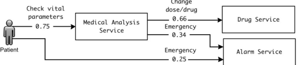
The Tele Assistance System (TAS) provides health support to patients in their home (Weyns & Calinescu, 2015). Patients wear a device that uses remote third-party services from health care, pharmacy, and emergency service providers. Figure 3 shows the TAS workflow that comprises different services. The workflow can be triggered to periodical measure the patient’s vital parameters and invoke a medical service for their analysis. Depending upon the analysis result a pharmacy service can be invoked to deliver new medication to the patient or change his/her dose of medication, or the alarm service can be invoked, dispatching an ambulance to the patient. The alarm service can also directly by invoked the patient via a panic button on the wearable device.
Figure 3. TAS workflow
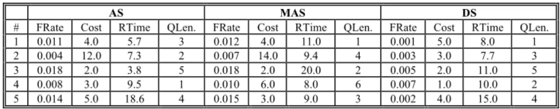
Multiple service providers provide concrete services for the Alarm Service (AS) Medical Analysis Service (MAS), and Drug Service (DS). Concrete services have a failure rate FRate, an invocation Cost, and a service time. The service time comprises two components: the response time RTime of invocations of a concrete service and the waiting time due to queues QLen with pending invocations. Table 1 shows the initial values as provided by the service providers. We assume that Cost
and RTime are fixed, while FRate and QLen are subject to change over time.
Patient Medical Analysis Service Alarm Service Drug Service 0.25 0.75 0.66 0.34 Emergency Change dose/drug Emergency Check vital parameters
Table 1. Third party service profiles for TAS
AS MAS DS
# FRate Cost RTime QLen. FRate Cost RTime QLen. FRate Cost RTime QLen.
1 0.011 4.0 5.7 3 0.012 4.0 11.0 1 0.001 5.0 8.0 1
2 0.004 12.0 7.3 2 0.007 14.0 9.4 4 0.003 3.0 7.7 3
3 0.018 2.0 3.8 5 0.018 2.0 20.0 2 0.005 2.0 11.0 5
4 0.008 3.0 9.5 1 0.010 6.0 8.0 6 0.007 1.0 10.0 2
5 0.014 5.0 18.6 4 0.015 3.0 9.0 3 0.002 4.0 15.0 4
As a default behavior, we assume that TAS selects a particular configuration of services, e.g. {AS3, MAS4, DS1}.
We consider two types of uncertainties in TAS. The first uncertainty is related to the different actions invoked to the system. As shown in Fig. 1, we assume that on average 75% of the requests are checks of vital parameters and 25% of the requests are emergency calls. After checking vital parameters, depending upon the result 66% of the requests invokes the drug service and 34% of the requests invoke the alarm service. However, these probabilities can change over time. The second uncertainty is related to the failure rates and queue length of services. Depending upon the network and other conditions the initial values of these characteristics are subject to change.
TAS should guarantee the following QoS requirements:
• R1. The assistance service invocations that fail to complete successfully should
be below 1.5% (per series of 1000 invocations).
• R2. The average cost for assistance service per invocation should be below 8.0
units.
• R3. The average service time for any patient should be less than 60 time units.
• R4. If requirements R1, R2, and R3 are satisfied, select the configuration with
minimum failure rate, service time, and cost in this order of priority.
• R5. If any of the requirements R1, R2 or R3 is not satisfied then gradually relax
requirements. If no configuration satisfies R1 then it can gradually be relaxed by 0.5% per step. Once R1 is satisfied, R2 can be increased gradually by 0.5
units, and subsequently R3 by 5 time units to find a configuration.
An offline analysis may find a configuration that supports the set of requirements. But to deal with the uncertainties associated with TAS, there is a need for adapting the current configuration at runtime based on the actual values of these uncertainties.
5.
Applying
RSMC
to TAS
In this section, we evaluate RSMC for a prototypical realization of the TAS example. We start with presenting the stochastic model of TAS. Then, we explain the verification queries for the requirements. Next, we provide initial results that show the feasibility of RSMC for this domain, and we conclude with results about the scalability of RSMC.
5.1.
Modeling
We model the TAS system using stochastic timed automata (STA). We use distinct models for the different quality requirements R1, R2, and R3. Using distinct models supports separation of concerns and allows to model precisely what is required to verify each requirement, which in turn leads to a reduced state space of the model that helps to perform simulations faster.
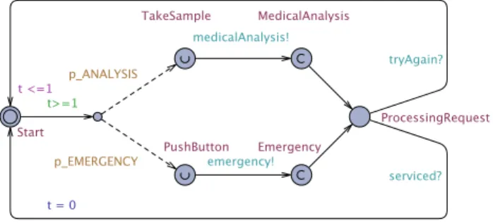
R1 models
We make a distinction between STA for the environment and the managed system. Figure 4 shows the environment model that represents the actions invoked to TAS. We use a scenario where each time tick either a sample of the vital parameters is taken from the user (with a probability value of p_ANALYSIS) or the user pushes the alarm button (with probability p_EMERGENCY, i.e., 1 – p_ANALYSIS). A sample is sent for analysis via the medicalAnalysis! signal, while pushing the alarm button triggers an emergency call via the emergency! signal. The probabilities of these actions are updated at runtime. After invoking an action, TAS processes the request. Once the service completes, the user is notified via the serviced? signal. If the service fails, the user is notified and can retry via the tryAgain? signal.
Figure 4. R1: Environment model
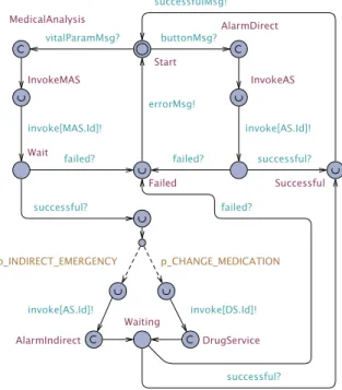
Figure 5 shows the model of the managed system. The managed system starts with assigning concrete services to the workflow for the simulation run with the function
assignServices(AS,MAS,DS) and then waits for the incoming requests from the
environment. Upon receiving a request for medical analysis or an emergency call, respectively the signals vitalParamMsg! or the buttonMsg! are sent to the workflow model. After invoking the workflow the request is processed in the Processing state until the successfulMsg? or errorMsg? signals are received, which triggers a notification to the Environment model via the serviced! or tryAgain! signal.
Figure 5. R1: Managed system model
Figure 6 shows the STA of assistance service representing the workflow of TAS. Upon receiving a service invocation signal from the managed system model, the corresponding service is called. In case of a failure, an errorMsg! is sent. In case of a successful invocation of the medical analysis service, the alarm service or drug service is called according to the probabilities associated with these services, i.e.,
p_INDIRECT_EMERGENCY and p_CHANGE_MEDICATION respectively.
Figure 6. R1: Assistance service
Figure 7 shows the STA for a concrete service. Before deployment, the automaton is initialized for each concrete service with a failure rate expressed as an integer ranging from 0 to 100. The automaton shows that a service waits for a signal from the assistance service. After receiving an invocation signal, depending upon failure
probability, the service fails or invoked successfully. If successful, the service responds with a successful! signal, otherwise, failed! signal is sent.
Figure 7. R1: Concrete service
R2 Models
R2 models are simplified versions of the R1 models, i.e., without the service failure behavior. For requirement R2, we measure average cost per invocation of assistance service, which is calculated without service failures.
Figure 8 shows the environment model of user behavior that sends requests for medical analysis and emergency service. After that, the user waits for serviced? signal before sending another request.
Figure 8. R2: Environment model
Figure 9 shows the model of the managed system for R2. Similar to the model of the managed system for R1, the model of the managed system for R2 starts with assigning concrete services to the workflow that are used for the simulation run using the function assignServices(AS,MAS,DS) and then waits for the incoming requests from environment. Upon receiving a request for medical analysis or an emergency call, respectively the signals vitalParamMsg! or the buttonMsg! are sent to the workflow model, and the model waits for execution of the request in the
Processing state until the done? signal is received, which triggers a notification to
Figure 9. R2: Managed system model
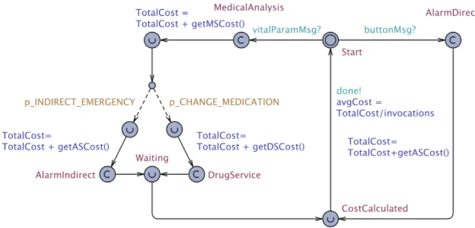
Figure 10 shows workflow model for R2 to calculate the estimated cost for using the assistance service. The total cost of an invocation is equal to the sum of the costs of the concrete services that are used. The total cost per invocation depends on the path that is taken in the workflow based on the type of request, i.e., buttonMsg! or
vitalParamMsg!. If the alarm service is directly invoked calculating the cost is
straightforward and equal to the actual cost of the concrete alarm service that is used
(getASCost()). If the medical analysis service is invoked the cost is calculated by
summing the cost of the concrete analysis service plus the cost of concrete alarm service or drug service, depending on the probabilities p_INDIRECT_EMERGENCY
and p_CHANGE_MEDICATION. Finally, the average cost is calculated using the
total number of invocations.
Figure 10. R2: Assistance service
R3 models
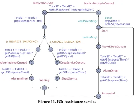
The models for of the environment and the managing system for R3 are the same as for R2 as shown in Figure 9 and Figure 10. Figure 11 shows the quality model to estimate service times. The service time per invocation is accumulated by the time the request has to wait in the queues plus the actual execution time, depending on the path that is taken.
Figure 11. R3: Assistance service
5.2.
Requirements
In this section, we explain how the adaptation requirements of TAS are realized (using Uppaal-SMC notation).
R1: Failure rate
R1 requires that the failure rate of assistance service should be less than 1.5% (over a series of 1000 invocations). To calculate the failure rate, we use the probability estimation property discussed in Section 2.1.
𝑃𝑟[<= 1](<> 𝐴𝑠𝑠𝑖𝑠𝑡𝑎𝑛𝑐𝑒𝑆𝑒𝑟𝑣𝑖𝑐𝑒.𝐹𝑎𝑖𝑙𝑒𝑑)
The actual failure rates of services and invocation probabilities of the models are updated at runtime. Then for each possible service configuration, this property is used with statistical model checker to calculate the failure rate of the assistance service.
R2: Cost per invocation
R2 requires that the cost of using the assistance service should be below 8 units per invocation. To that end, we use the simulation property discussed in Section 2.2 before.
The statistical model checker calculates the average cost of the assistance service over a time bound T. An important aspect that needs to be considered here is how many simulations are required to provide a confidence that the cost per invocation is close enough to the true cost. A smaller number of simulations will be performed faster but could introduce less accurate results; on the other hand, a large number of simulations will provide more accurate results, but require more verification time. To determine the required number of simulations, we used the relative standard error of the mean (RSEM). The standard error of the mean (SEM) quantifies how precisely a simulation result represents the true mean of the population (and is thus expressed in units of the data). The SEM takes into account the value of the standard deviation and the sample size. RSEM is SEM divided by the sample mean expressed as a percentage. For example, RSEM of 5% provides an accuracy with a SEM of +/- 0.5 units for a mean value of 10. Evidently, more accurate results (better estimates) require smaller RSEM values and thus more simulation runs. We used the following formula for calculating SEM, where 𝜎 represents standard deviation of the sample and N is the sample size:
𝑆𝑡𝑎𝑛𝑑𝑎𝑟𝑑 𝑒𝑟𝑟𝑜𝑟 𝑜𝑓 𝑚𝑒𝑎𝑛 𝑆𝐸𝑀 = 𝜎/ 𝑁
Once the SEM is calculated, the RSEM is calculated by dividing the SEM by the mean of the sample and multiplying by 100:
𝑅𝑒𝑙𝑎𝑡𝑖𝑣𝑒 𝑆𝐸𝑀= 100∗𝑆𝐸𝑀/x̄
In this report, we used accuracy levels of 5% and 10% for R2 and R3. To find out, how many simulations are required to get the required accuracies we performed an offline experiment. In particular, we took 20 randomly selected configurations to calculate the RSEM. Based on the results, 25 simulations are required for a RSEM of 10% and 100 simulations for 5%. For further information about the use of the RSEM for simulation queries, we refer the interested reader to (Weyns, 2016). The queries to measure the cost per invocation for 10% and 5% RSEM are respectively:
𝑠𝑖𝑚𝑢𝑙𝑎𝑡𝑒 1[<= 25]{𝐴𝑠𝑠𝑖𝑠𝑡𝑎𝑛𝑐𝑒𝑆𝑒𝑟𝑣𝑖𝑐𝑒.𝑎𝑣𝑔𝐶𝑜𝑠𝑡} 𝑠𝑖𝑚𝑢𝑙𝑎𝑡𝑒 1[<= 100]{𝐴𝑠𝑠𝑖𝑠𝑡𝑎𝑛𝑐𝑒𝑆𝑒𝑟𝑣𝑖𝑐𝑒.𝑎𝑣𝑔𝐶𝑜𝑠𝑡} R3: Service time
To measure average service time, for simulation we used the same RSEM values as used in R2. This gives the following queries:
𝑠𝑖𝑚𝑢𝑙𝑎𝑡𝑒 1[<= 25]{𝐴𝑠𝑠𝑖𝑠𝑡𝑎𝑛𝑐𝑒𝑆𝑒𝑟𝑣𝑖𝑐𝑒.𝑎𝑣𝑔𝑆𝑇𝑖𝑚𝑒}
𝑠𝑖𝑚𝑢𝑙𝑎𝑡𝑒 1[<= 100]{𝐴𝑠𝑠𝑖𝑠𝑡𝑎𝑛𝑐𝑒𝑆𝑒𝑟𝑣𝑖𝑐𝑒.𝑎𝑣𝑔𝑆𝑇𝑖𝑚𝑒} R4: Prioritize R1
R4 prioritizes the different quality properties. In particular, R4 requires that if there are multiple configurations available, then a configuration should be chosen based on the lower failure rate. In case, two or more configurations have the same failure
rate, then a selection should be made on the basis of service time. If service time is also same then a configuration with lower cost should be selected. The following algorithm is used to find the best configuration that fulfills the requirements:
double R1 = 0.015, R2 = 8.0, R3 = 60.0; Config findBestConfig(){
double bestFrate = MAX_VAL, bestCost = MAX_VAL, bestSTime = MAX_VAL; Config config, bestConfig = null;
int bestIndex = -1;
for (int i = 0; i < MAX_CONFIG; i++){ config = configurations[i];
if (config.FailureRate < R1 && config.Cost < R2 && config.STime < R3){
if (config.FailureRate < bestFR || (config.FailureRate == bestFR && config.STime < bestSTime) || (config.FailureRate == bestFR && config.STime == bestSTime && config.cost < bestCost)){ bestIndex = i; bestFR = config.FailureRate; bestCost = config.Cost; bestSTime = config.STime; } } } if (bestIndex != -1){ bestConfig = configurations[bestIndex]; } return bestConfig; }
Algorithm 1. Algorithm to find a best configuration
R5: Relax requirements
If there is no configuration found by algorithm 1 that satisfies requirements R1 to R3, then algorithm 2 is used to relax the requirements and find a configuration:
void applyRules(){
bestConfig = findBestConfig(); if (bestConfig == null){
r1Satisfied = checkR1Satisfied(R1, configurations) while(r1Satisfied == false){
R1+= 0.005;
r1Satisfied = checkR1Satisfied(R1, configurations) }
}
/* Now we are sure that R1 can be satisfied. try again to find any configuration which satisfies all requirements. now if still we have not find the bestConfiguration, then we need to increase gradually other requirements.*/
bestConfig = findBestConfig(); while(bestConfig == null){ R2 += 0.5; bestConfig = findBestConfig(); if (bestConfig == null){ R3 += 5; } bestConfig = findBestConfig(); } }
Algorithm 2. Algorithm to relax requirements
Algorithm 2 consists of two parts. The first part searches for configurations that satisfy R1. We check all the configurations and if no configuration satisfies R1, then we gradually relax R1 with 0.5%, until we find such a configuration(s). The second part searches for configurations that satisfy the other requirements. We check all the configurations and if no configuration satisfies R2 and R3, we gradually increase R2 and R3 by 0.5 unit and 5 time units respectively, until a configuration is found.
6.
Experiments
In this section, we evaluate the proposed RSMC approach using different scenarios of TAS. The evaluation consists of three parts: (1) the impact of different parameter settings for the verification queries of the different requirements, (2) the quality of adaptations for different settings, and (3) the scalability of our approach. For the second and third part, we include a comparison with runtime quantitative verification. We start with the experimental settings and then discuss the results of the experiments. All material is available for download via the ActivFORMS website: http://homepage.lnu.se/staff/daweaa/ActivFORMS/ActivFORMS.htm
6.1.
Experimental Settings
In this section, we describe the RSMC settings we used for the experiments and the experiment template we use to report the results.
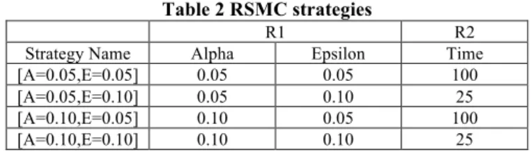
RSMC strategies
We use different RSMC strategies for the experiments, i.e. values for the parameters of the RSMC queries. Table 2 illustrates different parameter values for R1 & R2:
Table 2 RSMC strategies
R1 R2
Strategy Name Alpha Epsilon Time
[A=0.05,E=0.05] 0.05 0.05 100
[A=0.05,E=0.10] 0.05 0.10 25
[A=0.10,E=0.05] 0.10 0.05 100
[A=0.10,E=0.10] 0.10 0.10 25
Experiment Template
We use the following template to present the results of the experiments:
Experiment Name: Name of the experiment;
Purpose: Motivation for the experiment;
RSMC strategies: Any particular setting of RSMC used in the experiment; if the result of this experiment is presented as a graph, then the strategy name will be displayed as legend on the graph;
TAS settings: Any particular setting of TAS used in the experiment;
Measurements: Number of measurements taken;
Result: Results of experiment, usually displayed as a graph;
Conclusion: Brief discussion of the experiment conclusions.
6.2.
Properties of Verification Queries
In this section, we discuss experiments performed on each verification property.
Experiment Name: R1 verification
Description: In this experiment, we measure how different values of alpha and
epsilon affect the failure rate measured by the verification query for R1:
𝑃𝑟[<= 1](<> 𝐴𝑠𝑠𝑖𝑠𝑡𝑎𝑛𝑐𝑒𝑆𝑒𝑟𝑣𝑖𝑐𝑒.𝐹𝑎𝑖𝑙𝑒𝑑)
We also calculate the verification time to run this query (i.e., the number of runs performed by Uppaal-SMC) and measure the number of states of the model that are explored. In this experiment, we use one service configuration. Unlike numerical approaches, a statistical approach does not necessarily provide the same results for each invocation, but returns a confidence interval {Lower bound, Upper bound}. We report the value for R1 as the average of the confidence interval:1
𝐹𝑎𝑖𝑙𝑢𝑟𝑒 𝑅𝑎𝑡𝑒 =𝐿𝑜𝑤𝑒𝑟 𝐵𝑜𝑢𝑛𝑑 + 𝑈𝑝𝑝𝑒𝑟 𝐵𝑜𝑢𝑛𝑑
2
RSMC strategies: settings as Table 2, but values for R2 not applicable.
1
TAS settings: We use the configuration {AS1, MAS1, DS1} with default failure rates and probabilities from Table 1.
Measurements: 1000
Result:
Conclusion: The results show that lower alpha and epsilon values generate more efficient results (smaller box plots). However, the verification time increases with efficient results as a result of the increasing number of runs and explored states.
Experiment Name: R2 verification
Description: In this experiment, we measure how different values of time (T) affect the results of the cost measured by the verification query for R2:
𝑠𝑖𝑚𝑢𝑙𝑎𝑡𝑒 1[<= 𝑇 ]{𝐴𝑠𝑠𝑖𝑠𝑡𝑎𝑛𝑐𝑒𝑆𝑒𝑟𝑣𝑖𝑐𝑒.𝐶𝑜𝑠𝑡}
The query returns the average cost to invoke the assistance service for T invocations. By using different values of T, we want to determine how accurate cost is measured with 5% and 10% RSEM. We also want to measure the average verification time and how many runs and states are being explored. We have used only one TAS configuration in this experiment.
RSMC strategies: We use the following specific RSMC strategies:
R1 R2
Configuration Alpha Epsilon Time
10% N/A N/A 25 5% N/A N/A 100 R1 Verification 0.01 0.02 Avg =(L ow erBo un d+U pp erBo un d)/ 2 Failure Rate 0 5 10 15 20 T ime in mi lli se co nd s (ms) Verification Time 0.05 0.10 0.15 0.20 0.25 R un s in ki lo s (k) Runs 1 2 3 4 St at es in ki lo s (k)
RSMC strategy A=0.05,E=0.05 A=0.10,E=0.05 A=0.05,E=0.10 A=0.10,E=0.10 Explored States
TAS settings: {AS1, MAS1, DS1} with default values given in Table 1.
Measurements: 1000
Result:
Conclusion: The results show the invocation cost for 5% and 10% RSEM. There is significant difference in verification time and explored states for the two RSMC strategies, but memory usage is similar.
Experiment Name: R3 verification
Description: In this experiment, we measure how different values of time (T) affect the results of the service time measured by the verification query for R3:
𝑠𝑖𝑚𝑢𝑙𝑎𝑡𝑒 1[<= 𝑇 ]{𝐴𝑠𝑠𝑖𝑠𝑡𝑎𝑛𝑐𝑒𝑆𝑒𝑟𝑣𝑖𝑐𝑒.𝑎𝑣𝑔𝑆𝑇𝑖𝑚𝑒}
The query returns the average cost to invoke the assistance service for T invocations. Similar as for R2, we want to measure how accurate service time is measured with values that correspond to 5% and 10% RSEM, as well as the number of runs and the number of states being explored. We us one TAS configuration in this experiment.
RSMC strategies:
R1 R2
Configuration Alpha Epsilon Time
10% N/A N/A 25
5% N/A N/A 100
TAS settings: {AS1, MAS1, DS1} with default values given in Table 1.
Measurements: 1000 Result: 10% 5% 7.0 7.2 7.4 7.6 7.8 8.0 C ost p er in vo ca tio n Invocation Cost 10% 5% 0.0 0.5 1.0 1.5 2.0 T ime in mi lli se co nd s (ms) Verification Time 10% 5% 4.70 4.75 4.80 4.85 Me mo ry in me ga byt es (MB) Memory Usage 10% 5% 0.4 0.6 0.8 1.0 St at es in ki lo (K) Explored States R2 Verification
Conclusion: The results show the service time for 5% and 10% RSEM. Similar as for cost (R2) there is a significant difference in time and explored states for both RSMC strategies, but no relevant difference in memory usage.
Experiment Name: verify R4
Purpose: This experiment demonstrates that R1 is prioritized over R2 and R3.
RSMC strategies:
R1 R2
Strategy Name Alpha Epsilon Time
0.05 0.05 100
TAS settings: All service configurations as shown in Table 1.
Measurements: 1 Result: 10% 5% 33 34 35 36 37 38 Se rvi ce ti me in se co nd s Service time 10% 5% 0 1 2 3 4 T ime in mi lli se co nd s (ms) Verification Time 10% 5% 4.75 4.80 4.85 4.90 Me mo ry in me ga byt es (MB) Memory Usage 10% 5% 0.4 0.8 1.2 St at es in ki lo (K) Explored States R3 Verification 0.010 0.015 0.020 0.025 Failure rate Ave ra ge co st p er in vo ca tio n 4 6 8 10 12 14 16 18 Configuration Valid configuration Selected configuration 0.010 0.015 0.020 0.025 40 60 80 100 120 Failure rate Ave ra ge se rvi ce ti me
Conclusion: The verification results show that R1 is prioritized over R2 and R3 for the selected configuration, which illustrates that requirement R4 is satisfied. The algorithm selects the configuration with the lowest failure rate.
Experiment Name: verify R5
Purpose: This experiment demonstrates that R1 is prioritized over R2 and R3 when relaxation of the requirements is required.
RSMC strategies:
R1 R2
Strategy Name Alpha Epsilon Time
0.05 0.05 100
TAS settings: We used the following settings: the probability that the user pushes the emergency button is 0.27 (hence, the probability that the medical analysis service is called for is 0.73). The following service characteristics are used:
AS MAS DS
# FRate Cost RTime QLen. FRate Cost RTime QLen. FRate Cost RTime QLen.
1 0.013 4.0 5.7 2 0.014 4.0 11.0 2 0.002 5.0 8.0 1 2 0.006 12.0 7.3 5 0.007 14.0 9.4 5 0.005 3.0 7.7 4 3 0.019 2.0 3.8 3 0.020 2.0 20.0 4 0.006 2.0 11.0 1 4 0.009 3.0 9.5 2 0.011 6.0 8.0 2 0.009 1.0 10.0 4 5 0.014 5.0 18.6 2 0.015 3.0 9.0 1 0.003 4.0 15.0 4 Measurements: 1 Result:
Conclusion: The results show that Algorithm 1 could not find a configuration that satisfies the initial requirements. Compliant to requirement R5, Algorithm 2 relaxes some of the requirements. In this particular case, R2 is relaxed from 8.0 to 8.50 to select a configuration. 0.010 0.015 0.020 0.025 Failure rate Ave ra ge co st p er in vo ca tio n 4 6 8 10 12 14 16
18 ConfigurationValid configuration
Selected configuration 0.010 0.015 0.020 0.025 40 60 80 100 120 140 Failure rate Ave ra ge se rvi ce ti me
6.3.
Adaptation experiments
In this section, we discuss experiments related to adaptation of TAS.
Experiment Name: Adaptation of TAS
Purpose: We periodically adapt TAS after 1000 service invocations and measure the failure rate of TAS through the sliding window of 1000 service invocations. We also measure the adaptation time taken for different RSMC strategies.
RSMC strategies: The following strategies are used in the experiment
R1 R2
Strategy Name Alpha Epsilon Time
A=0.05,E=0.05 0.05 0.05 100
A=0.10, E=0.10 0.10 0.10 25
TAS settings: We have used the default settings of TAS specified in Table 1 and the behavior discussed in Section 6.1. For all experiments, we apply uncertainties to the quality properties of each service and the user behavior after 1000 invocations of the assistance service. The failure rate of each service and user behavior (direct invocation of emergency service) are updated based on a normal distribution with a standard deviation of 0.03 and 0.10 respectively, and the queue length of each service is randomly selected from between 1…5. The probabilities for invocations of the drug service after medical analysis remain the same in the experiments.
Measurements: To measure failure rates, we use a sliding window, which stores the latest 1000 service invocations, and measures the failure rate after each invocation. To measure the adaptation times, we used 20 measures for each RSMC strategy
Result:
Conclusion: The graph on the left hand side shows that the failure rates of TAS comply with the requirements for the setting with 5% RSEM (lower alpha and epsilon settings and the higher number of simulations), while the setting with 10% RSEM leads to some violations. The median of the average cost remains under the constraint of 8 units for both configurations, but both settings lead to some violations. Service times are similar, but the adaptation time is significantly lower for the setting with 10% RSEM. RQV guarantees the requirement for failure rates.
0.010 0.015 0.020 F ai lu re R at e 1 2 3 4 5 Ad ap ta tio n time (s) 30 60 90 120 Se rvi ce ti me 4 6 8 10 12 14 16 C ost RQV A=0.05,E=0.05,T=100 A=0.10,E=0.10,T=25
Cost and service time are similar as for RSMC, but at the cost of a significant higher adaptation time.
6.4.
Scalability Experiments
We check the scalability of our approach and compare it with RQV. For RQV, we have used an equivalent TAS model (for the specification, see Section 5.1).
Experiment Name: Scalability w.r.t. the number of concrete services of one type
Purpose: Measure adaptation times for anincreasing number of emergency services.
RSMC strategies: The following RSMC strategies are used in this experiment:
R1 R2
Strategy Name Alpha Epsilon Time
A=0.05,E=0.05,T=100 0.05 0.05 100
A=0.10,E=0.10,T=25 0.10 0.05 25
TAS settings: In this experiment, we use the services specified in Table 1. For the additional emergency services, failure rates and cost are provided randomly. The cost of each extra service is randomly selected between 1-15 units, a failure rate is selected between 0.01-0.02 and the service time is selected between 1.0-20.0.
Measurements: For each RSMC strategy and for RQV, we measure how many alarm services are supported up to 30 seconds. We show average results of five measurements of each adaptation time.
Result:
Conclusion: With RQV,up to 12 services are supported for adaptation times of 30 seconds. For RSMC, this is 40 and 100 respectively, depending on the RSMC strategy used. The results show that RSMC is more scalable than RQV with respect to an increasing number of services of one type. Furthermore, RSMC allows making a tradeoff between confidence and adaptation time (further improving scalability, but of course at the price of reduced confidence of the results).
Experiment Name: Scalability w.r.t. the number of concrete services of all types
Purpose: Measure adaptation times for anincreasing number of concrete services.
RSMC strategies: The following RSMC strategies are used in this experiment: 0
10 20
30
5 10 15 20 25 30 35 40 45 50 55 60 65 70 75 80 85 90 95 100 Number of emergency services
T ime in se co nd s RQV RSMCA=0.05,E=0.05,T=100 RSMCA=0.10,E=0.10,T=25
R1 R2
Strategy Name Alpha Epsilon Time
A=0.05,E=0.05,T=100 0.05 0.05 100
A=0.10,E=0.10,T=25 0.10 0.05 25
TAS settings: In this experiment, we measure the adaptation time by increasing the concrete services for each abstract service. Failure rates and cost for each additional service is provided randomly, similar to the previous experiment.
Measurements: For each RSMC strategy and for RQV, we measure how many concrete services are supported up to 10 minutes adaptation time. We take 5 measurements of each setting, and show the average in a graph.
Result:
Conclusion: The results show that RQV support adaptation for only 12 concrete services in 10 minutes, whereas with RSMC depending upon different strategies can support 24 to 34 concrete services for each abstract service.
Experiment Name: Scalability w.r.t. an increasing number of abstract services
Purpose: Measure adaptation times for anincreasing number of abstract services
RSMC strategies: The following RSMC strategies are used in this experiment:
R1 R2
Strategy Name Alpha Epsilon Time
A=0.05,E=0.05,T=100 0.05 0.05 100
A=0.10,E=0.10,T=25 0.10 0.10 25
TAS settings: In this experiment, we measure the adaptation time by increasing the number of abstract services. To that end, we used a workflow for the assistance service that invokes services sequentially, and if any of the services fail the assistance service fails. We have used three concrete services for each abstract service. Failure rates and cost are provided randomly as explained above.
Measurements: For each RSMC strategy and RQV, we measure the number of concrete services that are supported up to 15 minutes. The reported results are averages of 5 measurements. 0.0 2.5 5.0 7.5 10.0 5 6 7 8 9 10111213141516171819202122232425262728293031323334
Number of concrete services
T ime in mi nu te s RQV RSMCA=0.05,E=0.05,T=100 RSMCA=0.10,E=0.10,T=25
Result:
3
services services 4 services 5 services 6
RSMC
A=0.10, E=0.10, T=25 0.5 sec 4.0 sec 28.0 sec 3.04 min
RSMC
A=0.05,E=0.05, T=100 2.6 sec 18.9 sec 2.13 min 13.4 min
RQV 4.1 sec 59.4 sec 11.4 min not
measurable
Conclusion: Results shows that the adaptation time increases exponentially, both for RQV and RSMC. However, the RSMC strategies take less adaptation time as RQV and the gap increases with the number of abstract services. For 3 abstract services RSMC (A=0.05,E=0.05, T=100) is twice as fast as RQV, for 4 services RSMC is four times faster as RQV, and for 5 services the difference is almost a factor six. The difference between RSMC (A=0.05,E=0.05, T=100) and RSMC (A=0.10,E=0.10, T=25) is about a factor 4 and is constant for all configurations.
7.
Appendix: RQV
Models
This appendix presents the RQV models and queries we used to perform the experiments. The models and queries are equivalent to those we used for RSMC as described in Section 5.1. We created separate models for requirements R1-R3. Whenever an adaptation is required, first the values of all uncertainties of the models are assigned and then requirements R1-R3 are calculated for each configuration.
R1: Failure rate
We start with the probabilistic model we used for R1. We do not go into details, but refer the reader interested in the details about probabilistic models to: http://www.prismmodelchecker.org/manual/ThePRISMLanguage/Introduction
label "failed_tas" = result = -1; label "success_tas" = result = 1; module Environment x : [0..4] init 0; result : [-1..1] init 0; [] x = 0 -> p_ANALYSIS:(x'=1) + p_EMERGENCY:(x'=2); [medicalAnalysis] x = 1 -> (x'=3); [emergency] x = 2 -> (x'=3);
[tryAgain] x = 3 -> (x'=4) & (result'=-1); [serviced] x = 3 -> (x'=4) & (result'=1); [] x = 4 -> (x'= 4); endmodule module ManagedSystem m: [0..5] init 0; [medicalAnalysis] m = 0 ->(m'=1); [emergency] m = 0 -> (m'=2); [vitalParamMsg] m = 1 -> (m'=3); [buttonMsg] m = 2 -> (m'=3); [successfulMsg] m = 3 -> (m'= 4); [errorMsg] m = 3 -> (m'=5); [serviced] m = 4 -> (m'=0); [tryAgain] m = 5 -> (m'=0); endmodule
Property: The following property has been used to calculate failure rate: 𝑃=? [ 𝐹 "𝑓𝑎𝑖𝑙𝑒𝑑_𝑡𝑎𝑠" ] module AssistanceService service: [0..3] init 0; resultAS:[-1..1] init 0; serviceInvoked:bool; // Invoke medical service
[vitalParamMsg] service = 0 -> (service'=Medical) & (serviceInvoked' = false); // Invoke emergency
[buttonMsg] service=0 -> (service'=Alarm) & (serviceInvoked' = false); // invoke appropriate medical service
[invokeM1] service=Medical & MAS = 1 & (serviceInvoked = false) -> (serviceInvoked'=true); // Upon successful invocaiton call the alarm or drug service
[invokeD1] service=Drug & DS = 1 & (serviceInvoked = false) -> (serviceInvoked'=true); [invokeA1] service=Alarm & AS = 1 & (serviceInvoked = false) -> (serviceInvoked'=true); // Invocation to other medical, alarm and drug services here
// On Successful medical service, invoke drug or alarm service
[successfulM1] service = Medical & MAS = 1 & serviceInvoked -> p_CHANGE_MEDICATION : (service'=Drug)& (serviceInvoked' = false) + p_INDIRECT_EMERGENCY : (service'=Alarm) & (serviceInvoked' = false); // On successful invocation of alarm or drug services write the result
[successfulA1] service = Alarm & AS = 1 & serviceInvoked -> (resultAS' = 1) & (serviceInvoked' = false) & (service'=0);
[successfulD1] service = Drug & DS = 1 & serviceInvoked -> (resultAS'=1)& (serviceInvoked' = false) & (service'=0 // Receive successful messages from remaining services here
// Receive failure messages from services
[failedM1] service=Medical & MAS = 1 & serviceInvoked -> (resultAS'=-1)& (serviceInvoked' = false) & (service'=0); [failedA1] service=Alarm & AS = 1 & serviceInvoked -> (resultAS'=-1)& (serviceInvoked' = false) & (service'=0); [failedD1] service=Drug & DS = 1 & serviceInvoked -> (resultAS'=-1)& (serviceInvoked' = false) & (service'=0); // Receive failure messages from other remaining services
// Notify the managing system about success or failure [successfulMsg] resultAS=1 -> (resultAS'=1); [errorMsg] resultAS=-1 -> (resultAS'=-1); endmodule
module MedicalAnalysisService1 m1:[0..4] init 0;
[invokeM1] service = Medical & MAS = 1 -> (m1'=1); [] m1 = 1 -> 1-mas1FR:(m1'=2) + mas1FR:(m1'=3); [] m1 = 2 -> (m1'=4);
[successfulM1] m1 =4 -> (m1'=0); [failedM1] m1 = 3 -> (m1'=0); endmodule
R2: Cost
For calculating the cost per invocation of the assistance service, we used reward properties provided by the probabilistic model.
Property: The following property has been used to calculate cost per invocation: 𝑅{"𝑐𝑜𝑠𝑡"}=? [ 𝐹 "𝑠𝑢𝑐𝑐𝑒𝑠𝑠_𝑡𝑎𝑠" ]
module Environment x: [0..4] init 0;
// Let managed system do the initializations first
[] x = 0 & ASCost != 0 & MASCost != 0 & DSCost != 0 -> p_ANALYSIS : (x'=1) + p_EMERGENCY:(x'=2); [medicalAnalysis] x = 1 ->1.0: (x'=3); [emergency] x = 2 -> 1.0:(x'=3); [success] x = 3 -> (x'=4); [] x = 4 -> (x'= 4); endmodule label "success_tas" = x = 4; module ManagedSystem y:[0..4] init 0;
// Initialization of managed system []AS=1 & ASCost = 0 -> (ASCost'=AS1Cost); []MAS=1 & MASCost = 0 -> (MASCost'=MAS1Cost); []DS=1 & DSCost = 0 -> (DSCost'=DS1Cost); []AS=2 & ASCost = 0 -> (ASCost'=AS2Cost); []MAS=2 & MASCost = 0 -> (MASCost'=MAS2Cost); []DS=2 & DSCost = 0 -> (DSCost'=DS2Cost); []AS=3 & ASCost = 0 -> (ASCost'=AS3Cost); []MAS=3 & MASCost = 0 -> (MASCost'=MAS3Cost); []DS=3 & DSCost = 0 -> (DSCost'=DS3Cost); []AS=4 & ASCost = 0 -> (ASCost'=AS4Cost); []MAS=4 & MASCost = 0 -> (MASCost'=MAS4Cost); []DS=4 & DSCost = 0 -> (DSCost'=DS4Cost); []AS=5 & ASCost = 0 -> (ASCost'=AS5Cost); []MAS=5 & MASCost = 0 -> (MASCost'=MAS5Cost); []DS=5 & DSCost = 0 -> (DSCost'=DS5Cost); [medicalAnalysis] y = 0 -> (y'=1); [emergency] y = 0 -> (y'=2); [vitalParamMsg] y = 1 -> (y'=3); [buttonMsg] y = 2 -> (y'=3); [done] y = 3 -> (y'= 4); [success] y=4 -> (y'=0); endmodule
module AssistanceService z:[0..4] init 0;
[buttonMsg] z = 0 -> (z'=Alarm); [vitalParamMsg] z = 0 -> (z'=Medical);
[] z = Medical -> p_CHANGE_MEDICATION:(z'=Drug) + p_INDIRECT_EMERGENCY:(z'=Alarm); [] z = Alarm -> (z'=4); [] z = Drug -> (z'=4); [done] z = 4 -> (z'=0); endmodule rewards "cost" z = Alarm: ASCost; z = Medical: MASCost; z = Drug: DSCost; endrewards
R3: Service time
Following model has been used to calculate service time for RQV:
Property: The following property has been used to calculate service time: module patient x: [0..4] init 0; [] x = 0 -> p_ANALYSIS:(x'=1) + p_EMERGENCY:(x'=2); [medicalAnalysis] x = 1 ->1.0: (x'=3); [emergency] x = 2 -> 1.0:(x'=3); [success] x = 3 -> (x'=4); [] x = 4 -> (x'= 4); endmodule label "success_tas" = x = 4; module ManagedSystem y:[0..4] init 0; [medicalAnalysis] y = 0 -> (y'=1); [emergency] y = 0 -> (y'=2); [vitalParamMsg] y = 1 -> (y'=3); [buttonMsg] y = 2 -> (y'=3); [done] y = 3 -> (y'= 4); [success] y=4 -> (y'=0); endmodule
module AssistanceService z:[0..4] init 0;
[buttonMsg] z = 0 -> (z'=Alarm); [vitalParamMsg] z = 0 -> (z'=Medical);
[] z = Medical -> p_CHANGE_MEDICATION:(z'=Drug) + p_INDIRECT_EMERGENCY:(z'=Alarm); [] z = Alarm -> (z'=4);
[] z = Drug -> (z'=4); [done] z = 4 -> (z'=0); endmodule
rewards "service_time"
z = Alarm & AS=1 : (AS1QLen + 1) * as1Stime; z = Alarm & AS=2 : (AS2QLen + 1) * as2Stime; z = Alarm & AS=3 : (AS3QLen + 1) * as3Stime; z = Alarm & AS=4 : (AS4QLen + 1) * as4Stime; z = Alarm & AS=5 : (AS5QLen + 1) * as5Stime; z = Medical & MAS=1 : (MAS1QLen + 1) * mas1Stime; z = Medical & MAS=2 : (MAS2QLen + 1) * mas2Stime; z = Medical & MAS=3 : (MAS3QLen + 1) * mas3Stime; z = Medical & MAS=4 : (MAS4QLen + 1) * mas4Stime; z = Medical & MAS=5 : (MAS5QLen + 1) * mas5Stime; z = Drug & DS=1 : (DS1QLen + 1) * ds1Stime; z = Drug & DS=2 : (DS2QLen + 1) * ds2Stime; z = Drug & DS=3 : (DS3QLen + 1) * ds3Stime; z = Drug & DS=4 : (DS4QLen + 1) * ds4Stime; z = Drug & DS=5 : (DS5QLen + 1) * ds5Stime; endrewards
8.
Bibliography
Bulychev, P., David, A., Larsen, K. G., Mikučionis, M., Poulsen, D. B., Legay, A., & Wang, Z. (2012). UPPAAL-SMC: Statistical Model Checking for Priced Timed Automata. In proceedings QAPL 2012,EPTCS 85, pp. 1-16.
Calinescu, R., Ghezzi, C., Kwiatkowska, M., and R. Mirandola, R. (2012). Self-adaptive Software Needs Quantitative Verification at Runtime. Communications of
the ACM, 55(9), pp. 69–77.
Cheng B., et al. (2014). Using Models at Runtime to Address Assurance for Self-Adaptive Systems, [email protected]: Foundations, Applications, and Roadmaps, Lecture Notes in Computer Science, Springer.
Clarke, E. M., Faeder, J. R., Langmead, C. J., Harris, L. A., Jha, S. K., & Legay, A. (2008, October). Statistical Model Checking in BioLab: Applications to the Automated Analysis of T-Cell Receptor Signaling Pathway. In International Conference on Computational Methods in Systems Biology (pp. 231-250). Springer. David, A., Larsen, K. G., Legay, A., Mikučionis, M., & Poulsen, D. B. (2015). Uppaal SMC tutorial. International Journal on Software Tools for Technology Transfer, 17(4), 397-415.
de Lemos R., et al. (2013) Software Engineering for Self-Adaptive Systems: A Second Research Roadmap, Lecture Notes in Computer Science, Springer. Dobson, S. Denazis, S. Fernandez, A. Gati, D., Massacci, M. Nixon, P., Saffre, F., Schmidt, N., and Zambonelli, F. (2006). A Survey of Autonomic Communications,
ACM Transactions on Autonomous and Adaptive Systems, pp. 223- 259.
Garlan, D., Cheng, S. W., Huang, A. C., Schmerl, B., & Steenkiste, P. (2004). Rainbow: Architecture-based Self-adaptation with Reusable Infrastructure. Computer, 37(10), 46-54.
Hansen, J., Wrage, L., Chaki, S., de Niz, D., and Klein, M., (2015). Semantic Importance Sampling for Statistical Model Checking, European Joint Conferences
on Theory and Practice of Software, TACAS'15. Springer.
Hérault, T., Lassaigne, R., Magniette, F., & Peyronnet, S. (2004, January). Approximate Probabilistic Model Checking. In International Workshop on Verification, Model Checking, and Abstract Interpretation (pp. 73-84). Springer. Kephart, J. O., & Chess, D. M. (2003). The Vision of Autonomic Computing.
Computer, 36(1), 41-50.
Kramer, J., & Magee, J. (2007, May). Self-Managed Systems: an Architectural Challenge. In Future of Software Engineering, 2007. FOSE'07 (pp. 259-268). IEEE. Legay, A., Delahaye, B., & Bensalem, S. (2010). Statistical Model Checking: An Overview. In International Conference on Runtime Verification(pp. 122-135). Oreizy, P., Medvidovic, N., & Taylor, R. N. (1998, April). Architecture-Based Runtime Software Evolution. In Proceedings of the 20th international conference on Software engineering (pp. 177-186). IEEE Computer Society.
Weyns, D., & Iftikhar M. U. (2016). Model-based Simulation at Runtime for Self-adaptive Systems. Models at Runtime, Wurzburg, Germany. IEEE.
Weyns, D., Malek, S., & Andersson, J. (2012). FORMS: Unifying Reference Model for Formal Specification of Distributed Self-Adaptive Systems. ACM Transactions on Autonomous and Adaptive Systems (TAAS), 7(1), 8.
Weyns, D., & Calinescu, R. (2015, May). Tele Assistance: A Self-Adaptive Service-Based System Examplar. In Proceedings of the 10th International Symposium on Software Engineering for Adaptive and Self-Managing Systems (pp. 88-92). IEEE. Weyns, D., Bencomo, N., Calinescu, R., Camara, J., Ghezzi, C., Grassi, V., Grunske, L., Inverardi, P., Jezequel, J., Malek, S., Mirandola, R., Mori, M., and Tamburrelli, G. (2016) Perpetual assurances in self-adaptive systems. In Software
Engineering for Self-Adaptive Systems III. Lecture Notes in Computer Science,
Springer.
Younes, H. L. (2005). Verification and Planning for Stochastic Processes with Asynchronous Events. In proceedings of the 19th National Conference on Artificial Intelligence (pp. 1001-1002). AAAI Press.