UNIVERSIT
À
DELL'INSUBRIA
FACOLT
À
DI
ECONOMIA
http://eco.uninsubria.it
K. Passarin
Robust Bayesian estimation
2004/11
© Copyright K. Passarin
Printed in Italy in May 2004
Università degli Studi dell'Insubria
Via Ravasi 2, 21100 Varese, Italy
All rights reserved. No part of this paper may be reproduced in
any form without permission of the Author.
In questi quaderni vengono pubblicati i lavori dei docenti della
Facoltà di Economia dell’Università dell’Insubria. La
pubblicazione di contributi di altri studiosi, che abbiano un
rapporto didattico o scientifico stabile con la Facoltà, può essere
proposta da un professore della Facoltà, dopo che il contributo
sia stato discusso pubblicamente. Il nome del proponente è
riportato in nota all'articolo. I punti di vista espressi nei quaderni
della Facoltà di Economia riflettono unicamente le opinioni
degli autori, e non rispecchiano necessariamente quelli della
Facoltà di Economia dell'Università dell'Insubria.
These Working papers collect the work of the Faculty of
Economics of the University of Insubria. The publication of
work by other Authors can be proposed by a member of the
Faculty, provided that the paper has been presented in public.
The name of the proposer is reported in a footnote. The views
expressed in the Working papers reflect the opinions of the
Authors only, and not necessarily the ones of the Economics
Faculty of the University of Insubria.
Robust Bayesian Estimation
∗
Katia Passarin
†Abstract
This paper deals with the problem of robust estimation in a Bayesian context. We present an overview on some families of so-called robust distributions and we prove that they belong to the family of elliptical distributions. Accord-ing to this results, extensions to the multivariate case can be easily obtained. Moreover we propose criteria to assess when using a robust model is recom-mend and how to choose among estimates obtained with different models.
1
Introduction
The problem of building robust estimation procedures in a Bayesian context is an intriguing issue. In 1980 Box argues that to build efficient models, model robustifi ca-tion is required, “where by robustification I mean judicious and grudging elaboration of the model to ensure against particular hazard (..). Robustification becomes nec-essary when it is known that likely, but not easy detectable, model discrepancies can yield badly misleading analyses.”
In Bayesian literature wefind two ways to build robust procedures. Thefirst one is used within the global approach and applies when a large range is obtained for the functional. It aims to narrow the class of prior and/or sampling distributions down to the point where a satisfactory range is reached. We refer for example to Berger (1994), Liseoet al. (1996) and Morenoet al. (1996) for different ways of reducing the width of a class. A second way applies when normality is adopted for the sampling distribution. In Bayesian analyses this assumption is convenient in order to obtain analytical results for the posterior and it turns out to be often reasonable. However, in this case it is well known that the sensitivity of posterior quantities to observations is more pronounced and that only few atypical values in the sample heavily influence estimates. The reason for this fact has been found by many authors in light tails of the normal model adopted (Box and Tiao, 1968, 1992; Dawid, 1973; Zellner, 1976). Robustness with respect to outliers is achieved by choosing a so-calledrobust model. A robust model consists in a family of symmetric unimodal distributions enriched with ‘robustness’ parameters that control its shape. Therefore different univariate
∗This paper has been presented at the University of Insubria (Como) on the 22th of April 2004
and its publication in the working paper series of the Dep. of Economics of the U. of Insubria has been proposed by Prof. Mira, University of Insubria.
†Università della Svizzera Italiana, Istituto di Finanza, Facoltà di Economia, Via Buffi13, 6900,
Lugano, Switzerland. Email: [email protected]
unimodal heavy-tailed models have been proposed to replace the normal model (Box and Tiao, 1962; Ramsay and Novick, 1980; West, 1984; Albert et al., 1991) and the resulting posterior distribution becomes analytically intractable. However, this is not a limitation since the availability of faster and faster personal computers let us easily obtain estimates by means of Monte Carlo Markov Chain algorithms. Alternatively, normal approximations of the posterior distribution can be used (see for example Box and Tiao, 1992).
The goal of this paper is to propose Bayesian estimates which are robust against outliers, where we define an outlier to be an observation which is unlikely to have been generated by the assumed sampling model. For this purpose we follow the second way and we concentrate on posterior summaries with a normal sampling model assumption. However, many points have to be discussed. First, in many situations the presence of influential observations is not easily detectable (e.g. for the multivariate nature of data) and we may fail to recognize the need of a robust sampling model. It is possible to define measures that help us in deciding whether a robust model has to be adopted? Secondly, once we judge that a robust distribution is needed, how do we choose between different models? This paper discusses such points and it is organized as follows. In Section 2 we present an overview of some univariate robust models and we prove that they fall into the more general elliptical family. This result helps to easily generalize such distributions to the multivariate case and it is useful in many practical situations. The main contribution of the paper is to provide criteria to assess when adopting a robust model is recommended and how to choose between different distributions. We do this in Section 3. Different examples of robust Bayesian estimation are then implemented in Section 4. Finally conclusive remarks are given in Section 5.
2
Robust models
In this section we present different models which have been proposed in the litera-ture. First, we briefly introduce the class of elliptical distributions. Then we present an overview of some families of robust models. We show that such distributions fall into the class of elliptical distributions. Detailed proofs are given in Appendix 1. This result helps to easily generalize univariate distributions to the multivariate case and it is useful in many practical situations. Finally we propose criteria to assess the need of adopting robust models and to choose among them.
2.1
Elliptical distributions
The class of Elliptical Distribution (ED) is a family of symmetric distributions which includes among others the normal and the student−t. Moreover, it offers a simple way to generalize a univariate distribution to the multivariate case. It was
first introduced by Kelker (1970) and then studied by several authors (e.g. Fang and Anderson, 1990 and Gupta and Varga, 1993).
Definition 1 Let X be a k ×1 dimensional random vector whose distribution is
absolutely continuous. Then, X ∼ EDk(θ,Σ,Ψ) if and only if the p.d.f. of X has
the form f(X) =c· |Σ|−1/2g µ 1 2(X−θ) 0Σ−1(X −θ) ¶ (1)
where g and Ψ determine each other for a specified k. The function g is called the
density generator. Ψ is a function such that the characteristic function of X can be
written asϕX(t) = exp (it0θ)·Ψ
¡1
2t0Σt
¢
.
The condition R0∞uk2−1g(u)du < ∞ guarantees g to be a density generator.
Moreover, the normalizing constant can be obtained using the polar coordinates in several dimensions and is given by
c= Γ(k/2) (2π)k/2 ·Z ∞ 0 uk2−1g(u)du ¸−1 . (2)
A detailed prove of this result can be found in the paper by Landsman and Valdez (2003).
2.2
Main robust distributions
We now present location-scale families of distributions with tails decreasing to zero more slowly than the normal case. Parameters (µ, σ) represent the mean and the standard deviation of the distribution. We also give the form of the density generator when a distribution belongs to the elliptical family.
In 1962 Box and Tiao introduce the family of exponential power-series distribu-tions (EP S). Such a family is given by
( f(x|µ, σ, δ) =kδ ·σ−1·exp à −cδ· ¯ ¯ ¯ ¯x−σ µ ¯ ¯ ¯ ¯ 2 δ+1 ! , x∈<,−1< δ ≤1 ) , (3) where cδ = " Γ¡32(δ+ 1)¢ Γ¡12(δ+ 1)¢ # 1 δ+1 and kδ = £ Γ¡32(δ+ 1)¢¤1/2 (δ+ 1)£Γ¡1 2(δ+ 1) ¢¤3/2.
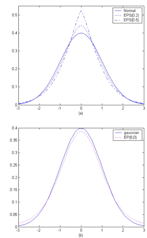
In EP S family µ is the location parameter, σ the scale parameter and δ can be regarded as a non-Normality parameter. For δ > 0 the distributions have heavier tails, forδ <0the distributions haveflatter tails than the normal form. This family is quite wide including as special cases the normal (δ= 0), the double exponential ( δ = 1) and the rectangular ( δ → −1) distributions. Since we are interested in distributions which are only lightly different from the normal one, we will choose small values forδ. In Appendix 1 we proved that (3) belongs to the elliptical family with density generatorg(u) = exp{−cδ·(2u)
1 δ+1}.
Some years later Ramsay and Novick (1980) measure the influence of a single observation xj on the posterior distribution by considering the derivative of the
logposterior with respect toxj. The latter turns out to be a function of a particular
quantity, named influence function of the likelihood (IFlik). They show that for a
certain symmetric family of distributions, which includes the normal, the IFlik is
unbounded. Hence, they propose a new family with bounded IFlik given by
© f(x|µ, σ, a, b) =ka,b· r(x) ·s(µ, σ)·exp © −ηa,b(d)ª, a >0, b >0ª, (4) where ηa,b(d) = ba12/bγ(2/b, a|d| b
), d is a measure of the distance of x from the location parameter µ, γ(p, z) is the incomplete gamma function and ka,b is the
normalizing constant. The normal distribution is obtained for a → 0. Therefore we would consider small values of this parameter. A peculiarity of this distribu-tion is that its tails do not decrease to zero as x tends to ∞. Indeed in this case
ηa,b(d)→ ba12/bΓ(2/b), which is a fixed quantity. The consequence is thatka,b has to
be computed in a region of integration with finite fixed limits. The choice of such limits is not so important as long as they are sufficiently far away from observed data. Once again, we prove that this family is an elliptical family with density generator g(u) = exp{−¡ba2/b¢−1
·R0a·(2u)b/2e−
tt2/b−1dt
}.
In 1991 Albert, Delampady and Polasek propose an extension of the EP S dis-tribution, called extended power distribution (EP). This family is given by
( f(x|µ, φ, c, λ) =kc,λ ·φ1/2·exp ( −c2·ρλ Ã 1 +φ(x−µ) 2 c−1 !) , c >1, λ≥0 ) , (5) where ρλ(v) = vλ−1 λ if λ >0 lim λ→0 vλ−1 λ = logv if λ = 0. ,
(µ, φ) are the location-scale parameters, (c, λ) are the robustness parameters and
kc,λ is the normalizing constant. The main advantage of (5) with respect to (3) is
that the former is differentiable everywhere. For this density we know that a relation of type σ2 = ν(φ) between the variance σ2 and parameter φ holds. Therefore we may alternatively express (5) as
f(x|µ, σ, c, λ) =kc,λ·σ−1· £ ν−1¡σ2¢ ·σ2¤ 1 2 ·exp ( −c 2 ·ρλ Ã 1 + ν −1(σ2) · σ2 c−1 µ x−µ σ ¶2!) .
If λ = 0 the relation is given by σ2 = (c−1)√2
(c−3)φ . If λ > 0 the relation can be found
only numerically. Different location-scale densities are included in this family, like the normal and the Student-t. The tails behavior is controlled by the parameter
λ. For 0 ≤ λ < 1 we get fatter tails, whereas for λ > 1 we get sharper tails than the normal case. For our purpose, we consider only the case λ = 0 and we choose the scale parameter φ so that the variance σ2 equals the variance of the
other distributions. Also this density belongs to the elliptical family with density generator g(u) = [ν−1(σ2) · σ2]12 ·exp ½ −c 2 ·ρλ µ 1 +2ν− 1(σ2)·σ2 c−1 u ¶¾ . 4
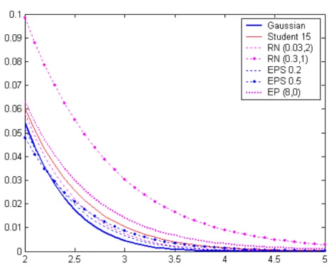
Another well known heavy-tailed distribution is the Student-t. The advantage of considering the previous families rather than the Student-t may be found in the wider choice of the elements in the class. In particular for distributions (4) and (5) two robustness parameters control the shape of the density function better. Fur-thermore the fact that for such models the normalizing constant has to be computed numerically does not represent a limitation. Indeed, robust estimation under these distributions is implemented through MCMC algorithms like Metropolis-Hastings (Hastings, 1970). In this way the normalizing constant cancels out in the accep-tance probability. Figure 1 and 2 show plots of the densities we presented in this section for different values of the robust parameters.
3
Criteria for robust estimation procedures
In this Section we establish rules of thumb for understanding when robust models have to be used and for choosing among different distributions.
In the literature robust models are adopted when the normal assumption appear inadequate. Typically this conclusion is drawn on the basis of a visual inspection of the data histogram, which is straightforward in the univariate dimension and can be replaced by nonparametric plot of the density in the bivariate case. When the dimension increases up tok (k > 2) reaching this task becomes hard. For this purpose local robustness measures described in Passarin (2004) are good tools. Such measures reveal also the presence of observations that have been unlikely generated by the assumed sampling model (outlier).
In this paper we concentrate on robust estimation of posterior summaries of type
TB =
R
ρ(θ)p(θ|x)dθ. To establish the need of using robust models, thefirst thing to do is to compute theSC (see Hampelet al., 1986) defined as
SC(z) = [TB(F z n)−TB(Fn−1)] 1 n ,
where Fn−1 = (x1, .., xn−1) is the empirical distribution of the sample of (n−1)
observations and Fz
n = (x1, .., xn−1, z) is the sample in which observation z has
been added. Such quantity evaluates the effect of moving one observation in the sample once a particular combination of prior/sampling distributions is fixed. If this measure diverges as z becomes bigger, a single observation has a potentially unbounded influence on the functional estimated value. However, this is not a sufficient reason to justify the use of a robust rather than a normal sampling model because influential observations there may be not present in the sample. In order to detect outliers we have to compute the local influence measure (briefly LI) for the sampling model. Such measure assesses the so-calledmodel or likelihood robustness
and evaluates the impact on the functional of a small contamination of the base sampling model. For posterior summaries, it can be written as
LI(G;TB, Fθ) =
X
j
mj(x;Π, Fθ, G)
m(x) [TB,j(Fθ, G)−TB], (6)
wheremj/mis the Bayes factor andTB,j(Fθ;G)is the posterior functional obtained
when the sampling distribution isG only for observationxj and Fθ for the others.
Alternatively, a relative local influence measure can be defined for the purpose of comparing different functionals (see Passarin, 2004) and it will be denoted byLI∗.
The Bayes factor in measure (6) captures the effect on the functional of choosing a contaminating model for observation j which is more adequate or less adequate than the base one with respect to observed data. If an outlier is present in the sample we expect that this quantity would assume values greater than 1 and the difference [TB,j(Fθ, G)−TB] would be not negligible, leading to a substantial value
of (6). In this case the use of a robust model is recommended for dumping the effect of extreme observations on the estimate.
Finally, measure (6) can also help in choosing the most appropriate robust model. If we adopt one of the distribution presented in Section 2.2, we guess that the corresponding LI measure for the sampling model displays quite a small value. Therefore a criterion of choice can be to adopt the distribution which displays the smallest value for (6). Furthermore, if such value is small itself, we achieve robustness both with respect to outliers and with respect to the sampling model. In the next Section we provide some examples on robust estimation procedures.
4
Examples of robust estimates
In this section we examine the same examples of Passarin (2004). Wefirst consider the mean of the posterior distribution in the univariate case with a sample drawn from a Gaussian distribution and we evaluate the effect of assuming a robust model when it is necessary and when it is not. Then we consider a Bayesian regression model using Ramsay and Novick’s data and we produce robust estimates of regres-sion coefficients. We use different heavy-tailed models for the sampling distribution to illustrate the robust estimation procedure.
4.1
Posterior mean
In the paper by Passarin (2004) the posterior mean was declared not robust with respect to observations. However, the small size of LI measures suggested that atypical observations were not present and robust estimation was not necessary. What would be the effect on the estimate of assuming a robust model in such a situation? We answer this question considering different sampling models whose densities are shown in Figures 1 and 2. The choice of robustness parameters has been made so that robust densities show heavier tails than the normal case (Figure 3).
By way of Random Walk Metropolis-Hastings algorithm the posterior distribu-tion has been computed. The prior is chosen to beN(0.5,1)and different sampling models are used. For each simulation100.000 runs have been launched. We explore graphically the convergence of the chain, which seems to be reached.
Estimates of posterior quantities are shown in Table 1. Analytical estimates, computed for the normal case, are reported above the Table. The concordance between analytical and numerical results supports convergence of our algorithm.
Estimates of posterior mean do not differ as much under different sampling models. However, the more we move away from normality, the more we loose in efficiency, since posterior variance increases. This trade-off between efficiency and dumping effect of outliers is typical of robust estimates. Moreover the concordance of posterior mean and median together with a visual insight show that the posterior distribution is still symmetric and unimodal for all distributions considered.
Table 2 shows local influence measures under different sampling models, com-puted by perturbing the base sampling distribution in the direction of aN(θ,10·σ2).
Derived LI∗ measures are small, supporting the fact that all models are
approxi-mately adequate to our data. Looking at all these elements together, we conclude that using a robust family of distributions when no extreme observations are present let us still correctly estimate the posterior mean.
In Table 3 and 4 we reproduce the same analysis introducing the observation
x4 = −5 in the sample. Numerically estimated posterior expectations are now
very different and change according to the robust model adopted. Tails inflation permits controlling the impact of the outlier on the estimate. Again the efficiency of estimates decreases as we move away from the normal case.
As expected, the measure of local influence for the normal sampling model ex-plodes, revealing inadequacy of the model to the data (LI∗ = 7.02·1025). This
explosion is due to the huge value that ratio rj assumes in correspondence to the
outlier (j = 4). Marginal likelihood m4(x;Π, Fθ, G) is much bigger than the base
marginal m(x), which means that data support distributions with heavy tails. In all robust models considered ranges both forTB,j and for rj are narrowed and local
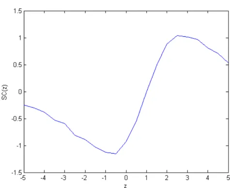
influence measure is reduced up to 0.35. Therefore to compute robust estimation we would adopt the RN distribution with parameters (0.3; 1). Robust estimate of the posterior mean is given by0.9270.
In the previous section we say that to achieve robustness with respect to outliers a robust sampling model has to be adopted. Therefore, in such a situation we expect theSC of posterior mean to be bounded for extreme observations. In Figure 4 we compute theSC for the selected robust model. The curve shows the expected behavior.
4.2
Bayesian Linear Regression
We now consider a Bayesian linear regression. We use the same data set employed by Ramsay and Novick (1980) and we study the impact that both a test of verbal intelligence and a test of performance intelligence have on dichotic listening task1. Bayes estimate of regression coefficients are found to be extremely sensitive to obser-vations. Moreover the local influence measure with respect to the sampling model reveals that the normal distribution is not so adequate (Passarin, 2004). In this section we will derive robust estimates of regression coefficients.
We consider different robust sampling models and compute the posterior dis-tribution with200.000 runs of the Metropolis-Hastings algorithm. Obtained Bayes
1We choose a normal prior distribution with the same parameters used by Rambsay and Novick
(1980).
estimates are shown in Table 5. The value of coefficients changes substantially ac-cording to different models while the standard error increases only a little. The substantial difference with normal estimates is clear forβb2. In this case the relation between the dichotic listening task and the test of performance intelligence changes from negative to slightly positive.
In order to choose robust estimates we compute local influence measures of re-gression coefficients for the sampling distribution. Table 6 shows the results. All robust models lead an improvement in terms of reducing the value ofLI∗ measures,
in particular the density proposed by Ramsay and Novick. Robust estimates of re-gression coefficients are therefore given bybβrobBayes = (0.6637,0.0082,37.6231)0. Such values are expected to be robust against influential points. Figure 15 shows the SC ofbβrobBayes. The improvement for regression coefficients estimates is clear since all the curves become bounded.
5
Conclusive remarks
In this paper we review some families of so-called robust distributions and we prove that they belong to the more general elliptical family. According to this result, mul-tivariate robust distributions can be easily obtained. Moreover we propose criteria to assess when the use of a robust model is recommend and how to choose between different distributions. First, the SC has to be computed for the estimator of in-terest. If a single observation plays a potentially unbounded influence, it is crucial to determine whether influential observations are present in the sample. For this purpose we use the local influence measure proposed in Passarin (2004). The exam-ples show both that the size of this measure becomes substantial when outliers are present and that adopting a robust model leads to estimates on which the effect of outlying observations is dumped. Moreover, the use of a robust family of distribu-tions when no extreme observadistribu-tions are present let us still obtain correct estimates. Obtained robust estimates behave well since the corresponding SC is bounded for extreme observations. Finally, the local influence measure for the sampling model provides also a criterion for choosing among different robust estimates. An interest-ing matter for future research on the field would be to include prior distributions also for robustness parameters of robust models.
References
[1] Albert, J., Delampady, M., Polasek, W. (1991), A class of distributions fro robustness studies,Journal of Statistical and Planning Inference, 28, 291-304. [2] Berger, J. O. (1994), An Overview of Robust Bayesian Analysis (with
discus-sion),Test, 3, 1, 5-124.
[3] Box, G. E. P. (1980), Sampling and Bayes’inference in scientific modelling and robustness, Journal of Royal Statistical Society, 143, 4, 383-430.
[4] Box, G. E. P., Tiao, G. (1962), A further look at robustness via Bayes’s theorem,
Biometrika, 49, 419-432.
[5] Box, G. E. P., Tiao, G. (1992),Bayesian Inference in Statistical Analysis,Wiley, New York.
[6] Dawid, A. P. (1973), Posterior expectations for large observations, Biometrika, 60, 664-666.
[7] Fang, K. T., Anderson, T. W. (1990), Statistical Inference in Elliptically
Con-toured and Related Distributions, Allenton Press Inc., New York.
[8] Gupta, A.K., Varga, T. (1993), Elliptically Contoured Models in Statistics, Netherlands, Kluwer Academic Publishers.
[9] Hampel, F. R., Ronchetti, E. M., Rousseeuw, P. J., Stahel, W. A. (1986),Robust
Statistics: The Approach Based on Influence Functions, Wiley, New York.
[10] Hastings, W. K. (1970), Monte Carlo sampling methods using Markov chains and their applications, Biometrika, 57, 97-109.
[11] Kelker, D. (1970), Distribution theory of spherical distributions and location-scale parameter generalization, Sankhya, 32, 419-430.
[12] Z., Landsman and E., Valdez (2003), Tail conditional expectation for elliptical distributions,North American Actuarial Journal, Vol. 7, No. 4, October 2003.
[13] Liseo, B., Petrella, L., Salinetti, G. (1996), Bayesian robustness: an interactive approach, Bayesian Statistics 5, (J. O. Berger et al., eds), 661-666, Oxford University Press, Oxford.
[14] Moreno, E., Martìnez, C., Cano, J. A. (1996), Local robustness and influence of contamination classes of prior distributions (with discussion), in Bayesian
Robustness (J. O. Berger et al., eds), IMS Lecture Notes - Monograph Series,
29, 137-154. Hayward: IMS.
[15] Passarin, K. (2004), Measures of local robustness for posterior summaries,
Tech-nical report n. 10, University of Insubria, Varese, Italy.
[16] Ramsay, J. O., Novick, M. R. (1980), PLU robust Bayesian decision theory: point estimation,Journal of the American Statistical Association,75, 372, 901-907.
[17] Rìos Insua, D., Ruggeri, F. (2000),Robust Bayesian Analysis, Springer-Verlag, New York.
[18] West, M. (1984), Outlier models and prior distributions in Bayesian linear regression, Journal of Royal Statistical Society (Series B), 46, 3, 431-439. [19] Zellner, A. (1976), Bayesian and non-Bayesian analysis on the regression model
with multivariate Student-t error terms, Journal of the American Statistical
Association,71, 400-405.
6
Appendix 1
In this appendix we prove that some well known univariate distributions belong to the elliptical family. Let’s define the variable u = 1
2
¡x−µ
σ
¢2
. The density func-tion of an elliptical distribufunc-tion can be written in the form f(x) = c·σ−1
·g(u),
where c = 2−1/2hR0∞u−12g(u)du
i−1
is the normalization constant. Any variable with density function of this form is said to be elliptically distributed. The exten-sion to the k−variate case is straightforward. In this case X is a k ×1 random vector andu = 1
2(X−µ)
0 Σ−1(X
−µ). The denstiy function is given by f(X) =
c· |Σ|−1/2g(u) and the normalization constant by c = Γ(k/2)
(2π)k/2 hR∞ 0 u k 2−1g(u)du i−1 . For a shorter notation, we denote the integralR0∞u−12g(u)du byI.
Normal distribution
IfX ∼N(µ, σ2), then it belongs to ED family with density generator
g(u) =e−u.
The integral I is given by
I =
Z ∞
0
u−12e−udu=Γ(1/2) =√π,
and the normalization constant is c= (2π)−1/2.
Student-t distribution
IfX ∼t(µ, σ2, p), then it belongs to ED family with
g(u) = µ 1 +2·u p ¶−(1+p)2 . IntegralI is given by I = Z ∞ 0 u−12 µ 1 +2·u p ¶−(1+p)2 du = √ 2πΓ¡1 +p2¢ √pΓ¡1+p 2 ¢ = √pπ ·Γ¡p2¢ √ 2·Γ¡1+2p¢, since with Γ(1 +z) =zΓ(z) if z >0.
The normalization constant is then given by
c = 2−1/2 √ 2·Γ¡1+2p¢ √pπ ·Γ¡p2¢ = Γ ¡1+p 2 ¢ Γ¡p2¢ (pπ) −1/2 . 11
Exponential Power-Series distribution
IfX ∼EP S(µ, σ, δ), then it belongs to ED family with
g(u) =e−cδ·(2u)(δ+1)
−1
.
Let’s make a riparametrization of the type s= (δ+ 1)−1 andr =cδ.
Then integral I is given by
I = Z ∞ 0 u−12e−r·(2u) s du = 21/2r−2s1 Γ µ 1 + 1 2s ¶ = 2 −1/2 s r −2s1 Γ µ 1 2s ¶ , and c = 2−1/22 1/2s ·r2s1 Γ¡21s¢ = s r 1 2s Γ¡21s¢ = £ Γ¡32(δ+ 1)¢¤1/2 (δ+ 1)£Γ¡12(δ+ 1)¢¤3/2 =kδ.
Ramsay and Novick’s distribution
IfX ∼RN(µ, σ, a, b), then it belongs to ED family with
g(u) = exp à −¡b·a2/b¢−1· Z a·(2u)b/2 0 e−tt2b−1dt ! , a >0, b >0. IntegralI, given by I = Z ∞ 0 u−12e−(b·a 2/b)−1·Ra·(2u)b/2 0 e− tt2b−1 dt du,
cannot be computed analitically.
However, considering the integral in the exponent, the following relation holds Z a·(2u)b/2 0 e−tt2b−1dt≤a·(2u)b/2e−t∗t 2 b−1 ∗ , where t∗ = maxt ³ e−tt2b−1 ´
>0 because the function is define on R+.
IntegralI can be written as I ≤ Z ∞ 0 u−12e−(b·a 2/b)−1·a·(2u)b/2e−t∗t2b−1 ∗ du = 212κ− 1 bΓ µ 1 +1 b ¶ <∞, with κ=b−1a2/b−1e−t∗t 2 b−1 ∗ .
Therefore,g is the density generator and the Ramsay and Novick’s distribution belongs to the elliptical family.
Extended Power distribution
IfX ∼EP (µ, σ, a, b), then it belongs to ED family with
g(u) =£ν−1¡σ2¢ ·σ2¤ 1 2 exp ½ −2c ·ρλ µ 1 +2 ν −1(σ2) · σ2 c−1 u ¶¾ . IntegralI, given by I =£ν−1¡σ2¢ ·σ2¤ 1 2 · ·Z ∞ 0 u−12exp ½ −c2·ρλ µ 1 + 2ν −1(σ2) · σ2 c−1 u ¶¾ du ¸ ,
can be computed analitically only forλ = 0. In this case we have
σ2 = (c−1) √ 2 (c−3)φ =⇒φ= (c−1)√2 (c−3)σ2 , and I = " (c−1)√2 (c−3)σ2 σ 2 #1 2 Z ∞ 0 u−12 exp ( −c 2log à 1 + 2 σ 2 (c−1) (c−1)√2 (c−3)σ2 u !) du = " (c−1)√2 (c−3) #1 2 Z ∞ 0 u−12 à 1 + 2 √ 2 (c−3) u !−c2 du = · (c−1)π 4√2 ¸1 2 Γ¡c 2 −1 ¢ Γ¡2c¢ <∞. 13
Table 1: Posterior estimates (standard error) under different sampling models. M CM C simulations with 100.000 runs. Analitical calculations in the normal case are above the table.
TB(Fθ) median σ2post Normal 0.9862 (0.0021) 0.9858 0.0625 Student-t (15) 0.9875 (0.0022) 0.9872 0.0697 EP S(0.2) 0.9996 (0.0021) 1.0037 0.0639 EP S(0.5) 1.0038 (0.0022) 1.0149 0.0669 EP (8; 0) 0.9953 (0.0023) 0.9966 0.0764 RN(0.03; 2) 0.9798 (0.0022) 0.9803 0.0699 RN(0.3; 1) 0.9663 (0.0027) 0.9737 0.1020 TB= 0.9857, σ2post = 0.0625
Table 2: Local influence measures of the posterior mean with respect to the sampling distribution under different sampling models. M CM C
simulations with 100.000 runs. The contaminating family is e
Gθ ={N(θ,10·σ2)}. Analitical calculations in the normal case
are above the table.
LI∗³Geθ;TB, Fθ ´ range TB,j(Fθ, Gθ) range rj Normal 0.0065 [0.8111; 1.1584] [0.3864; 0.6978] Student-t (15) 0.0123 [0.8151; 1.1606] [0.4049; 0.7203] EP S(0.2) 0.0183 [0.8083; 1.1654] [0.3869; 0.7553] EP S(0.5) 0.0249 [0.8119; 1.1785] [0.3872; 0.8356] EP (8; 0) 0.0162 [0.8129; 1.1571] [0.3434; 0.6910] RN(0.03; 2) 0.0173 [0.8112; 1.1583] [0.4023; 0.7017] RN(0.3; 1) 0.0553 [0.8058; 1.1146] [0.4920; 0.7440] range TB,j(Fθ, Gθ) = [0.8149; 1.1611], range rj = [0.3871; 0.6995] 14
Table 3: Posterior estimates (standard error) under different sampling models
M CM C simulations with 100.000 runs. Analitical calculations in the normal case are above the table. Contaminated sample.
TB(Fθ) median σ2post Normal −0.4384 (0.0018) −0.4392 0.0469 Student-t (15) 0.8032 (0.0023) 0.8067 0.0754 EP S(0.2) 0.0407 (0.0024) 0.0464 0.0825 EP S(0.5) 0.5207 (0.0024) 0.5295 0.0832 EP (8; 0) 0.8805 (0.0024) 0.8857 0.0823 RN(0.03; 2) 0.9776 (0.0022) 0.9761 0.0703 RN(0.3; 1) 0.9270 (0.0027) 0.9309 0.1028 TB =−0.4395, σ2post = 0.0476
Table 4: Local influence measures of the posterior mean with respect to the sampling distribution under different sampling models. M CM C
simulations with 100.000 runs. The contaminating family is e
Gθ ={N(θ,10·σ2)}. Analitical calculations in the normal case
are above the table. Contaminated sample.
LI∗³Geθ;TB, Fθ ´ range TB,j(Fθ, Gθ) range rj Normal 7.02·1025 [ −0.943; 0.804] [0; 2.49]·1025 Student-t (15) 91.9854 [ 0.572; 0.921 ] [0; 3.07]·103 EP S(0.2) 2.52·1016 [−0.460; 0.801] [0; 1.43]·1015 EP S(0.5) 6.50·107 [ 0.104; 0.965 ] [0; 1.13] ·108 EP (8; 0) 3.4226 [0.6841; 1.0256] [ 0.19; 21.88 ] RN(0.03; 2) 147.8905 [−0.071; 0.582] [0.39; 878.17] RN(0.3; 1) 0.3508 [0.6721; 1.0482] [ 0.39; 2.07 ] range TB,j(Fθ, Gθ) = [−0.947; 0.804], range rj = [0; 2.62]·1025 15
Table 5: Bayes Estimates (standard error) of regression coefficients under different sampling models. M CM C simulations with 200.000 runs. Analitical calculations in the normal case are above the table.
Regression coefficients
β1 β2 β3 normal 0.7455 −0.0716 38.1791 (0.0006) (0.0006) (0.0492) RN (0.05,2) 0.6637 0.0082 37.6231 (0.0008) (0.0009) (0.0577) EP S (0.2) 0.7051 −0.0290 37.6690 (0.0007) (0.0007) (0.0515) student (15) 0.6677 0.0067 37.4549 (0.0022) (0.0023) (0.1449) EP (5,0) 0.5836 0.0716 38.6109 (0.0009) (0.0008) (0.0691) b βBayes = [0.7458,−0.0734,38.3505]
Table 6: Relative local influence measures of regression coefficients with respect to the sampling distribution under different models.
M CM C simulations with 100.000 runs.
LI∗(G;T B, F)relative to β1 β2 β3 normal 43.14 471.41 5.82 RN (0.05,2) 0.14·10−5 5.94 ·10−5 0.15 ·10−5 EP S (0.2) 0.11·10−2 0.79·10−2 0.12·10−2 student (15) 7.32 173.14 0.30 EP (5,0) 0.91 2.34 0.14 16
Figure1: Plots of normal and robust densities: (a) Student-t and (b) RN distri-butions.
Figure 2: Plots of normal and robust densities: (a)EPS and (b) EP distributions.
Figure 3: Plot of the thickness of tails in normal and robust models.
Figure 4: Sensitivity curve of the posterior mean under a RN(0.3,1) sampling model. M CM C simulations with 100.000 runs.
Figure 5: Sensitivity curve of regression coefficients under a RN(0.05,2) sam-pling model. M CM C simulations with 100.000 runs.