Geosciences Faculty Publications and Presentations
Department of Geosciences
7-1-2015
Forecasting the Response of Earth’s Surface to
Future Climatic and Land Use Changes: A Review
of Methods and Research Needs
Jennifer L. Pierce
Boise State University
Michael J. Poulos
Boise State University
This work is provided under a Creative Commons Attribution-NonCommercial-NoDerivs 3.0 license. Details regarding the use of this work can be
found at:
http://creativecommons.org/licenses/by-nc-nd/4.0/
.
Earth's Future
is published by Wiley on behalf of the American Geophysical Union.
Copyright restrictions may apply. doi:
10.1002/2014EF000290
1Department of Geosciences, University of Arizona, Tucson, Arizona, USA,2Division of Earth and Ocean Sciences,
Nicholas School of the Environment, Duke University, Durham, North Carolina, USA,3Department of Geosciences, Boise
State University, Boise, Idaho, USA,4Department of Geology, University of Vermont, Burlington, Vermont, USA,5School
of Natural Resources and the Environment, University of Arizona, Tucson, Arizona, USA,6Department of Geosciences,
Idaho State University, Pocatello, Idaho, USA,7British Geological Survey, Environmental Sciences Centre, Nottingham,
UK,8Department of Civil Engineering, St. Anthony Falls Laboratory, University of Minnesota, Minneapolis, Minnesota,
USA,9School of Earth and Space Exploration, Arizona State University, Tempe, Arizona, USA,10Department of
Geography, Texas A&M University, College Station, Texas, USA,11Desert Research Institute, Reno, Nevada, USA,
12Department of Civil and Environmental Engineering, Duke University, Durham, North Carolina, USA,13Department of
Civil, Architectural, and Environmental Engineering, University of Padova, Padova, Italy,14Department of Earth and
Environment, Franklin & Marshall College, Lancaster, Pennsylvania, USA,15Department of Geological Sciences,
University of North Carolina, Chapel Hill, North Carolina, USA,16Department of Geology, Utah State University, Logan,
Utah, USA,17Division of Earth and Environmental Sciences, Los Alamos National Laboratory, Los Alamos, New Mexico,
USA,18College of Earth, Ocean, and Atmospheric Sciences, Oregon State University, Corvallis, Oregon, USA,
19Department of Geology, University of Cincinnati, Cincinnati, Ohio, USA,20Department of Geological Sciences,
University of Colorado, Boulder, Colorado, USA,21Department of Civil Engineering, University of Idaho, Boise, Idaho,
USA
Abstract
In the future, Earth will be warmer, precipitation events will be more extreme, global mean
sea level will rise, and many arid and semiarid regions will be drier. Human modifications of landscapes
will also occur at an accelerated rate as developed areas increase in size and population density. We now
have gridded global forecasts, being continually improved, of the climatic and land use changes (C&LUC)
that are likely to occur in the coming decades. However, besides a few exceptions, consensus forecasts do
not exist for how these C&LUC will likely impact Earth-surface processes and hazards. In some cases, we
have the tools to forecast the geomorphic responses to likely future C&LUC. Fully exploiting these models
and utilizing these tools will require close collaboration among Earth-surface scientists and Earth-system
modelers. This paper assesses the state-of-the-art tools and data that are being used or could be used to
forecast changes in the state of Earth’s surface as a result of likely future C&LUC. We also propose
strate-gies for filling key knowledge gaps, emphasizing where additional basic research and/or collaboration
across disciplines are necessary. The main body of the paper addresses cross-cutting issues, including the
importance of nonlinear/threshold-dominated interactions among topography, vegetation, and sediment
transport, as well as the importance of alternate stable states and extreme, rare events for understanding
and forecasting Earth-surface response to C&LUC. Five supplements delve into different scales or
pro-cess zones (global-scale assessments and fluvial, aeolian, glacial/periglacial, and coastal propro-cess zones) in
detail.
1. Introduction
1.1. Problem Statement
Many of the most significant effects of future climatic and land use changes (C&LUC) will occur on Earth’s
surface, which we consider to be synonymous with the critical zone [e.g.,
Anderson et al.
, 2008] and includes
Supporting Information:
• Supporting Information S1
Corresponding author:
J.D. Pelletier, [email protected]
Citation:
Pelletier, J. D. et al. (2015), Forecasting the response of Earth’s surface to future climatic and land use changes: A review of methods and research needs,Earth’s Future,3, 220–251,
doi:10.1002/2014EF000290. Received 9 DEC 2014 Accepted 22 MAY 2015
Accepted article online 26 MAY 2015 Published online 14 JUL 2015
© 2015 The Authors.
This is an open access article under the terms of the Creative Commons Attribution-NonCommercial-NoDerivs License, which permits use and distri-bution in any medium, provided the original work is properly cited, the use is non-commercial and no modifica-tions or adaptamodifica-tions are made.
the near-surface environment where humans obtain, produce, and consume air, water, and food necessary
for life. The delicate balance of human and ecosystem prosperity on Earth’s surface is challenged by climatic
variability, climate change, and unsustainable human activities.
The community of Earth-surface scientists (including, but not limited to, geomorphologists, hydrologists,
physicists, and applied mathematicians who work on landform evolution) has developed powerful
concep-tual and mathematical models for how Earth’s surface and near-surface environments are likely to respond
to and feed back on potential future C&LUC. For example, models have been developed that reproduce
observed recent changes in arctic permafrost landscapes [e.g.,
Plug and West
, 2009], aeolian dune systems
[e.g.,
Pelletier et al.
, 2009], and the response of coastal and river systems to sea level rise [e.g.,
Marani et al.
,
2007;
Fagherazzi et al.
, 2012] and land use change [e.g.,
Kirwan et al.
, 2011]. In many cases, however, these
models have not yet been systematically applied to forecasting landscape changes over large regions, which
limits their potential impact.
Earth-system modelers, in contrast, excel at working at the global scale. They have successfully represented
the key physical and chemical processes occurring in the atmosphere and oceans within their Earth System
Models (ESMs). However, ESMs have been less successful at representing some Earth-surface processes,
including the lateral redistribution of water, sediment, and nutrients near Earth’s surface. For example, land
models (for hydrometeorology, climate, and carbon cycle studies) often assume a globally uniform soil
depth (e.g., 2 m in
Gochis et al.
[2010]) above bedrock. Even the use of an unconfined aquifer in land models
implicitly assumes a global constant bedrock depth [e.g.,
Lawrence et al.
, 2011]. The land model components
of ESMs solve the governing equations for subsurface water flow in the vertical direction only, even though
water moves in all three directions in the subsurface [e.g.,
Miguez-Macho and Fan
, 2012]. Riverine sediment
flux, an important control on biogeochemical processes in wetlands, is another important component of
land surface processes not adequately accounted for in current ESMs. Given these limitations of current
ESMs, there is much to be gained if Earth-surface scientists and Earth-system modelers collaborate more
closely to assess the impacts of likely future C&LUC on human health, safety, and resource sustainability.
More basic research is also needed to further develop and refine Earth-surface response models so that
they can be applied to forecasting changes in the state of Earth’s surface in response to likely future C&LUC.
Quantitative modeling of Earth-surface processes and testing and calibration of models against data are
still in a relatively early stage of development compared with the advanced state of General Circulation
Models (GCMs) that comprise the atmospheric and oceanic components of ESMs. As such, the Earth-surface
scientific (ESS) community needs additional time and resources to develop models that accurately forecast
how some Earth-surface processes will respond to likely future C&LUC. Alluvial rivers, for example, tend to
aggrade when the ratio of sediment supply to transport capacity increases, and they tend to incise when
that ratio decreases [e.g.,
Bull
, 1991]. However, forecasting whether an alluvial river will aggrade or incise
in response to future C&LUC scenarios is complicated by the fact that the relationships among sediment
supply, transport capacity, rainfall, and vegetation cover are incompletely known. Similarly, we cannot yet
forecast whether future climate change will lead to an overall increase or decrease in dust emitted to the
atmosphere. Partly, this inability reflects the uncertainty in whether greater water use efficiency in a world
of higher atmospheric CO
2concentrations will outweigh the negative effect of limited water availability
in areas undergoing desertification. Our inability to forecast whether the future will be more or less dusty
also reflects the uncertainty associated with the relationship between vegetation cover and wind erosion.
More vegetation cover leads to higher turbulent stresses near the ground and hence may be expected to
increase rates of wind erosion. However, vegetation cover also acts to protect the underlying surface from
erosion, and the trade-offs between providing protection and causing higher turbulent shear stresses need
to be further resolved. To better forecast how dust emissions will change under future C&LUC scenarios, the
portion of the ESS community working on wind erosion must also collaborate more closely with scientific
communities working to predict future groundwater levels [e.g.,
Scanlon et al.
, 2006] and the vegetation
response to climate change in arid and semiarid regions [
Munson et al.
, 2011].
Natural experiments in the response of Earth-surface processes to C&LUC are constantly playing out across a
wide range of timescales from human to geological, and across a wide variety of process zones. Such natural
experiments provide essential data for developing and testing conceptual and mathematical models of
how geomorphic systems will respond to likely future C&LUC. In all cases, landform responses are known
From the perspective of modern climatic changes, high-level governmental discussions now acknowledge
that some amount of human-induced change is occurring and more change is inevitable. As a consequence,
significant effort is being steered toward the development of adaptation strategies. At the same time,
cli-mate scientists are acknowledging that a critical aspect of clicli-mate is its variability (particularly the increased
frequency of extreme events) rather than its mean value [e.g.,
Katz and Brown
, 1992]. Therefore, the need to
develop adaptation strategies requires a rigorous understanding of how landscapes respond to both the
mean and the variability of C&LUC. In turn, the state of Earth’s climate depends in part on the response of
landscapes to C&LUC. That is, the behavior of Earth’s surface feeds back on the climate system in ways that
are currently underrepresented in ESMs. Thus, a rigorous understanding of landscape response to external
forcings is important in the contexts of both adaptation and mitigation to climate change.
In this paper, we argue that, first, ESMs have simplified representations of many Earth-surface processes and
characteristics that could be improved with greater involvement of the ESS community in developing the
next generation of ESMs. Second, many of the consequences of future C&LUC are felt locally and will depend
sensitively on local topography, soil characteristics, vegetation cover, the degree of human disturbance, etc.
Improving our ability to forecast Earth-surface hazards will thus require that the ESS community improve
its ability to (1) work at larger (i.e., regional and global) scales and (2) develop forecasts (and hindcasts, to
test models against measurements) that use the forcing variables’ output by ESMs. Third, understanding
and forecasting future landscape responses will require that the nonlinearities and threshold-dominated
nature of Earth-surface systems be honored and better quantified. Fourth, a better understanding of the
feedbacks among vegetation, sediment transport, and topographic change is central to improved
fore-casting in all Earth-surface process zones; hence, collaboration among geomorphologists, geographers,
hydrologists, ecologists, and Earth-system modelers is needed.
1.2. Structure of This Review
In Section 2, we describe the nature of Earth-surface processes and hazards and their relationship to
C&LUC forcing variables, rank Earth-surface hazards in terms of their relative risk to society, explain how
Earth-surface processes and hazards relate to C&LUC forcing variables, and present a global map of where
particular types of surface processes are likely to be dominant. Section 3 discusses opportunities for spatially
explicit global-scale assessments of future changes in Earth’s surface. Section 4 highlights the importance
of nonlinearity, tipping points, and alternate stable states in Earth-surface systems. Section 5 emphasizes
the importance of the couplings among vegetation, sediment transport, and topography in forecasting
future landscape states. Section 6 argues for the importance of long timescales and natural experiments in
the geologic record in validating landscape response models before they can be used for forecasts. Section
7 discusses how landscape response models can be useful for evaluating alternative mitigation strategies.
Section 8 summarizes our recommendations how the ESS and broader geoscientific research communities
could work to improve forecasts of Earth-surface response to likely future C&LUC. We also include five
supplements that address specific scales and process zones. Text S1, Supporting Information, expands on
Section 3 and reviews the global gridded forecasts currently available from the ESM community that the
ESS community could use now to forecast Earth-surface responses to likely C&LUC. Text S1 also provides
exemplar models and data that have been used or could be used to perform global-scale assessments of
landscape response to C&LUC. Texts S2–S5 provide exemplar models and data that are being used or could
be used to forecast landscape responses within the hillslope/fluvial, glacial/periglacial, aeolian, and coastal
process zones, respectively. These supplements serve several purposes. They identify (1) the Earth-surface
processes within each process domain that are most sensitive to C&LUC, (2) the models and data that have
been or could be used to forecast Earth-surface responses to C&LUC, and (3) the key knowledge gaps and
the suggested pathways for filling them, including the development of coupled process-based models,
leveraging off of community-based code repositories/portals such as the Community Surface Dynamics
Modeling System (CSDMS) and greater collaboration across disciplines.
2. The Nature of Earth-Surface Processes and Hazards
The hazards associated with Earth-surface processes include acute events (e.g., floods) in addition to more
chronic events such as soil loss and the associated loss of food production potential. Examples of
societally relevant landscape properties in need of better forecasting include:
1. the elevation of the land surface, including its changes in space and time (i.e., subsidence, river
aggradation/incision, coastal erosion, etc.),
2. the fluxes of sediment and nutrients (as well as contaminants such as metals that impact water quality)
laterally across Earth’s surface,
3. the frequency and magnitudes of landslides, floods, dune encroachment, and other hazards related to
mobile water and sediment at or near Earth’s surface, and
4. particulate matter (PM) concentrations in the atmosphere, including those associated with fugitive
dust.
Not all Earth-surface hazards and/or changes in societally relevant properties pose an equal risk to society.
Therefore, it is useful to identify the most significant hazards to provide guidance on which hazards should
be prioritized for the development of improved forecasting tools. The risk associated with these hazards can
also be divided into a direct and an indirect risk. A direct risk is associated with loss of life and property. An
indirect risk is one that does not directly threaten a large number of lives or properties but may have
catas-trophic effects in concert with another process (e.g., the greenhouse effect). An example of an indirect risk
is the potential release of CO
2and methane into the atmosphere associated with thawing permafrost and
loss of ground ice, thus accelerating the greenhouse effect. In our ranking, we focused primarily on direct
risks. The ranking is subjective, but it is broadly consistent with order-of-magnitude estimates of the
finan-cial risk posed by these different types of hazards [e.g.,
Tol
, 2002, 2009]. We believe that future Earth-surface
hazards can be approximately ranked in terms of their potential impact as follows: (1) coastal erosion and
inundation, (2) river flooding and channel change, (3) water resource impacts (drought, desertification, and
water quality), (4) erosion and soil loss (including mass wasting and wildfire hazards), and (5) cryosphere
impacts (progressive thaw or melt in the cryosphere).
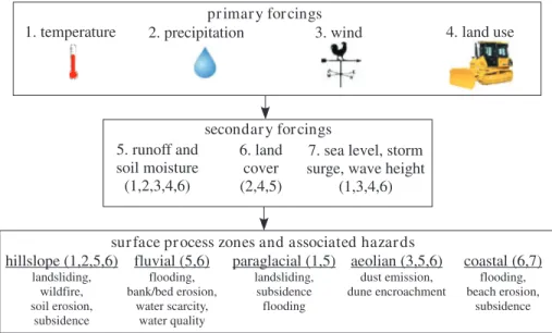
One challenge of forecasting Earth-surface responses to C&LUC is the fact that land surface processes
depend sensitively on secondary drivers related to but distinct from the basic variables of C&LUC. Figure 1
illustrates how different Earth-surface process types relate to the primary C&LUC variables of
temper-ature, precipitation, wind, and land use (including their mean values and their variability over a range
of timescales). Secondary variables include runoff and infiltration (i.e., hydrology), land cover (including
changes in the natural vegetation cover of landscapes and human disturbance, e.g., ecology and human
geography), and the coastal zone forcings of sea level, storm surge, and wave heights. While the effects of
climate hazards such as heat waves and droughts involve fairly direct linkages with primary climate
vari-ables, forecasting Earth-surface processes and hazards requires the translation of primary forcing variables
into secondary forcing variables before any forecasting can be done. The relationships among primary and
secondary variables are, in some cases, clear. For example, warming of the polar regions and continued
extraction of fluids from deltaic regions will drive relative sea level rise in many regions. In other cases,
the relationships are less clear. For example, how precipitation changes are likely to alter land cover in the
future is complex and incompletely understood. As such, Figure 1 underscores the need for collaboration
among specific geoscientific research communities, including among geomorphologists and hydrologists,
ecologists, and the human geographers who forecast land cover changes.
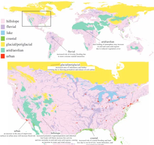
The types of Earth-surface processes and the associated hazards that dominate landscape response to
C&LUC vary regionally and globally (Figure 2). Glacial/periglacial zones are defined in Figure 2 as those with
mean annual temperatures less than 0
∘
C as determined using the WorldClim database [
Hijmans et al.
, 2005].
Increasing temperatures in such regions are likely to drive land subsidence due to thawing permafrost,
leading to a release of soil carbon that feeds back on the global climate system. Aeolian/arid areas are
hillslope (1,2,5,6)
landsliding, wildfire, soil erosion, subsidencefluvial (5,6)
flooding, bank/bed erosion, water scarcity, water qualityparaglacial (1,5)
landsliding, subsidence floodingaeolian (3,5,6)
dust emission, dune encroachmentcoastal (6,7)
flooding, beach erosion, subsidencesur face pr ocess zones and associated hazar ds
(1,3,4,6)
(2,4,5)
(1,2,3,4,6)
Figure 1. Conceptual diagram illustrating the linkages among the primary C&LUC forcing variables, secondary forcing variables (i.e., those that depend on the primary forcing variables but involve additional ecohydrologic and/or anthropogenic processes), and the main types of Earth-surface processes and their associated hazards. The numbers indicate dependencies. For example, the secondary forcings of sea level, storm surge, and wave height (#7) depend on global temperature changes (#1, e.g., melting polar ice), wind speeds (#3, e.g., stronger winds lead to greater storm surges and wave heights), land use (#4, e.g., fluid extraction from deltaic sediments can drive subsidence that contributes to relative sea level rise), and land cover (#6, e.g., changes in vegetation cover that can modify storm surges, dune mobility, etc.).
defined to be those with less than 200 mm a
−1of rainfall. Dust emission from such areas may increase in the
future due to increased aridity and reduced vegetation cover. Fluvial areas are delineated by routing
hypo-thetical extreme flows through the global 30-arc-second-resolution SRTM-derived DEM [
Farr et al.
, 2007]
augmented with ASTER GDEMV2 data where SRTM data were unavailable. Such areas are likely to
experi-ence more frequent flooding in response to future increases in precipitation intensity. However, changes
in sediment supply from hillslopes could cause valley floors to incise, thus decreasing flood risk in areas
adjacent to valley floors. Coastal areas are considered to be areas within 10 m of sea level. Many of these
areas will experience an increase in the frequency and magnitude of flooding and erosion, particularly in
areas where land subsidence is occurring simultaneously with the rise in global mean sea level. Urban areas
are mapped based on the Global Land Cover database [
Hansen et al.
, 1998]. As the population densities of
these areas increase, it is likely that peak flood discharges will be greater due to the lower infiltration rates
of impervious surfaces relative to natural surfaces. Hillslope areas are those not included in any of the other
process zones. On hillslopes in arid and semiarid regions, increased potential evapotranspiration and fuel
loads will likely trigger larger and more severe wildfires resulting in increased rates of soil erosion.
The thresholds of mean annual temperature, rainfall, and elevation that define the boundaries between
the process zones in Figure 2 are not unique. By presenting Figure 2, we are not suggesting that there is a
unique global map of process dominance. Rather, we are proposing that there is value in mapping regional
“hotspots” where landscapes are likely to be most sensitive to certain types of C&LUC. Such a map will be
useful in focusing research in those hotspots. In some cases, the hotspots of landscape response may occur
at the boundaries between process domains. For example, it is reasonable to expect that land degradation
(e.g., hillslope gullying, valley floor incision) is most likely to occur in semiarid regions that transition to arid
regions, rather than in areas that are already arid.
3. Opportunities for Spatially Explicit Global-Scale Assessments of Future
Changes in Earth’s Surface
The ESS community has a long and successful tradition of investigation at scales from individual hillslope
segments to the scale of whole watersheds. However, the ESM community necessarily works at the global
scale. One of the challenges of integrating process models and data from the ESS community into ESMs
glacial/periglacial
hillslope
fluvial
lake
coastal
arid/aeolian
fluvialincreased risk of riverine flooding due to more extreme rainfall intensities
glacial/periglacial
increased rates of subsidence and further warming due to thawing permafrost and release of soil carbon
hillslope
increased potential evapotranspiration and inherited fuel loads will likely increase fire activity and tree mortality in arid and semi-arid regions, causing
an increase in water and wind erosion
coastal
increased risk of coastal flooding and land loss due to sea-level rise, storm intensities, and
associated wave heights
arid/aeolian
dust loading of atmosphere may increase in arid and semi-arid regions due to reduced vegetation cover
urban
urban
an increase in the area of impervious surfaces in urban areas will increase flood risk
Figure 2.Map of dominant surface process zones, along with examples of the hazards and potential changes in hazards under future C&LUC scenarios. See text for a description of the criteria used to define each zone.
is the disparate scales at which most (though certainly not all) Earth-surface scientists and Earth-system
modelers work. Earth-system modelers require data and process models that have global coverage and are
globally applicable. Many Earth-surface scientists do not develop data or models with such global
applica-bility in mind. In this section, we argue for enhanced collaboration between the ESS and ESM communities.
Readily available data for future climates include near-surface temperature (and its daily and seasonal
variability), precipitation (and its event-scale and seasonal variability), potential evapotranspiration, and
near-surface wind speeds. Readily available data for future land use changes include changes in the
percent area (within 1
∘
x 1
∘
pixels) that will likely transition among crop, pasture, urban, primary (actively
disturbed), and secondary (previously disturbed but recovering) land use types. In order to make forecasts
of the Earth-surface response to C&LUC, the ESS community must further develop predictive Earth-surface
response models so that they work with available input data for future C&LUC scenarios. At the same
time, the ESS community needs to collaborate with Earth-system modelers and the climate and
geogra-phy communities to provide the most appropriate and useful inputs for Earth-surface response models.
For example, future vegetation states have been predicted, but these data usually predict vegetation
type only. Few Earth-surface response models are designed to work with vegetation type. Instead, many
existing models work with leaf area index (LAI) [e.g.,
Pelletier
, 2012] or other quantitative measures of
vegetation cover such as percent bare area. As such, the ESS community should collaborate more closely
with Earth-system modelers and the climate and geography communities to ensure that data products are
being produced that meet the needs of their models.
>10
4
yield (t km
–2
yr
–1
)
<10
2
10
3
sediment yield (anthropogenic effects excluded)
B
>10
5
<10
3
10
4
sediment yield (agricultural effects included)
yield (t km
–2
yr
–1
)
Figure 3. (a) Color map of the natural/pre-dam sediment yield as quantified by the model ofPelletier[2012]. (b) Sediment yield with agricultural effects included.
In this section, we use riverine sediment flux (or yield, defined as flux in mass per unit time divided by
drainage basin area) as an example of an Earth-surface process for which global-scale models exist that
could be used in the near future to forecast changes in response to likely future C&LUC. Quantifying
sed-iment yield in rivers has been a central topic in geomorphology for at least a century. Sedsed-iment yields
influence biogeochemical processes in wetlands [
Reddy et al.
, 2000]. Most predictive models for global
sed-iment yield focus on the suspended load component of the total load, which is the dominant component
of the total load for most large rivers.
Pelletier
[2012] developed a model that includes mean monthly
pre-cipitation, soil texture, and vegetation cover (quantified as LAI) explicitly (Figure 3). Sediment yield in this
model increases in direct proportion to average rainfall and decreases exponentially with increasing LAI.
It is straightforward to include the effects of agriculture in the
Pelletier
[2012] model, at least in a
simpli-fied way, as an example of how the land use changes could be explicitly included in current land surface
response models. Figure 3b illustrates the impact of modern agriculture on long-term average sediment
yields, assuming that croplands are areas of bare undisturbed ground in the model framework of
Pelletier
[2012]. This is a simplified approach because croplands are bare only part of the time. Neglecting plant cover
during the growing season likely leads to an overprediction of sediment yield, but this effect is somewhat
counteracted by the fact that cropland soils are disturbed by tillage, thus reducing their shear strength
rela-tive to bare undisturbed surfaces. When agriculture is included in the model, the region of largest sediment
yields in the U.S. shifts from the western U.S. to the eastern U.S. and the average sediment yield increases
by a factor of approximately 30, consistent with the findings of
Wilkinson and McElroy
[2007].
The challenge of quantifying the geomorphic responses to land use changes reflects the uncertainty in both
how sediment yield relates to land use and how land use should be quantified for input into models. Existing
global gridded datasets for land use predict the locations and density of transitions between primary land
and agricultural land, but it remains unclear how best to quantify the relationships between erodibility and
land use type. The effects of land use changes have been incorporated into empirical models for hillslope
sediment yields such as the Universal Soil Loss Equation (USLE) [
Wischmeier and Smith
, 1978]. The effects of
dams in storing sediments released from uplands have not been well quantified on a regional or global basis,
but the effect is substantial. Despite the recent order-of-magnitude increase in soil erosion in the eastern
U.S., the flux of sediment reaching the oceans is lower today than it has been in the past, indicating that
large volumes of sediment are being stored within the fluvial system [e.g.,
Walter and Merritts
, 2008;
Wisser
et al., 2013].
Syvitski and Milliman
[2007] included anthropogenic effects on sediment yield with drainage
basin–specific coefficients that depended on population density and GNP per capita. Additional research
is needed to identify how best land use/land cover data types can be used to quantify sediment yield.
4. Crosscutting Importance of Nonlinearity, Tipping Points, Alternate States, and
Uncertainty Propagation
Earth-surface systems are typically controlled by nonlinear and/or threshold-dominated responses to
changes in external forcings [e.g.,
Schumm
, 1979]. These nonlinearities imply that landscape responses
to ongoing and likely future C&LUC will be both amplified and difficult to predict. Here, we provide a
discussion of the basic concepts of nonlinear dynamical system theory [
Strogatz
, 2001], which provides an
essential framework for understanding Earth-surface response to likely future C&LUC.
Nonlinear systems respond at a variable rate to changes in external forcings. These responses can gradually
amplify the forcing, and/or they can include thresholds or “tipping points” that mark abrupt changes in the
forcing–response relationship. Nonlinear relationships between forcing and response lead to
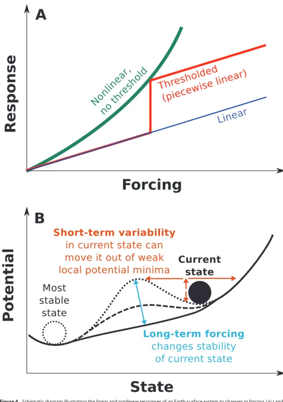
dispropor-tional responses to possibly subtle changes in forcing (Figure 4a), while feedbacks among processes
gov-erning system dynamics are often responsible for threshold responses to C&LUC (Figure 4a) and for driving
some systems into one of multiple alternative equilibrium states, with the associated potential for sudden
landscape/ecosystem transitions from one state to another (Figure 4b). Positive feedbacks have important
implications for Earth-surface science [e.g.,
Murray et al.
, 2008] (producing, for example, drainage network
development [
Rinaldo et al.
, 1998], conversion of alpine glaciers into debris-covered rock glaciers [
Scherler
et al.
, 2011], and river avulsions [
Slingerland and Smith
, 1998]), including these forms of rapid change and
instability in the face of gradual shifts in C&LUC.
An example of gradual amplification of a forcing change is dust entrainment, which is a major player in
Earth’s energy balance (because dust is a radiatively important aerosol) and exerts a significance influence
on human health. Dust entrainment scales approximately with the shear velocity exerted on the surface to
the third power and also depends nonlinearly on moisture/water table depth [e.g.,
Pelletier
, 2006].
Landslid-ing provides an example of a threshold-dominated behavior, in which slow soil creep can give way to
catas-trophic failure [
Ritter et al.
, 1999]. Bed load sediment transport rates relate to turbulent bed shear stresses in
a way that is both nonlinear and threshold dominated [
Gomez and Church
, 1989]. These nonlinear responses
make landscapes highly sensitive to C&LUC. In the southwestern U.S., for example, a transition from
wood-land to desert scrub species within elevation zones from approximately 800–1800 m above sea level caused
an order-of-magnitude increase in sediment supply from watersheds during the Pleistocene-to-Holocene
transition that triggered two downstream cycles of river and alluvial fan aggradation, incision, and renewed
aggradation [
Pelletier
, 2014]. In recent decades, small increases in springtime temperatures have
exponen-tially increased wildfire size and severity [
Westerling
et al., 2006], consistent with the measured correlation
between modest warming and dramatically increased burn extent and severity in the western U.S. through
the Holocene [
Pierce et al.
, 2004]. In many semiarid areas of the western U.S., drought-stressed forests will
not recover from vapor pressure deficits that manifest in non-replacement following disturbances such as
fire and insect infestations [
Williams et al.
, 2012]. This suggests that a vegetation-type conversion similar
in scope to vegetation changes recorded at the Pleistocene-to-Holocene transition [
Whitlock and Bartlein
,
1997] may be ongoing now, with important consequences for flood probabilities and soil sustainability.
Recent studies of tidal marsh dynamics highlight the importance of multiple stable states, and the
associ-ated potential for instability. For example, vegetation stabilizes tidal marshes by dissipating wave energy
and producing and trapping sediment. However, once sea level rise is sufficiently rapid enough to
out-pace this sediment production, marshes may be rapidly submerged and converted into sub-tidal platforms
Figure 4. Schematic diagram illustrating the linear and nonlinear responses of an Earth-surface system to changes in forcing. (a) Land surface systems in the presence of a positive feedback can present several competing states. (b) Illustrates the case of a system with two possible stable states. Shifts can occur because of short-term variability in the forcing (weather) overcoming the energy barrier separating the two coexisting states or because long-term changes in the forcing (climate) change the shape of the potential defining the available stable states, making one of the states disappear and leading the system to occupy the surviving lower energy stable state.
[
Marani et al.
, 2010]. In addition, recent modeling suggests that increasing storm frequency or the rate of
sea level rise can shift barrier islands from a regime with a single stable state featuring high dunes and
com-plex ecosystems into a regime in which a wave-swept, low topography state is an alternate possibility—or
even into a regime in which the high-dune state is no longer possible.
ESMs predict an increase in hydrologic variability as a result of human-induced global warming [
IPCC
, 2007,
2013], which should lead to enhanced geomorphic change [
Lane
, 2013]. However, uncertainties in future
landscape forcings obtained from climate models may translate into large uncertainties in forecasts of
future Earth-surface states due to nonlinear and possibly threshold-dominated geomorphic responses.
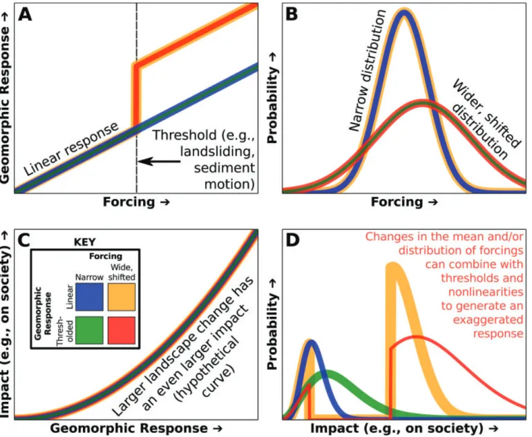
Figure 5 illustrates the propagation of uncertainty from forcing forecasts to Earth-surface-system responses
and finally to impacts on humans and infrastructure for two contrasting cases of linear and threshold
responses, assuming Gaussian distributions of uncertainty (Figure 5b). If the geomorphic response is
threshold dominated (Figure 5a), the distribution of responses is partitioned into two very distinct sets
of likely responses: both minor and major geomorphic responses may become plausible, thus increasing
the degree of uncertainty of the forecast (Figure 5d). The projected impact of the Earth-surface response
(e.g., on ecosystems or infrastructure; Figure 5c) must be combined with the probability distribution of
plausible geomorphic responses to statistically characterize the risk (Figure 5d). These schematic examples
underscore how essential it is to understand the linear/nonlinear nature of the processes at play in the
Earth-surface system in order to determine, and correctly interpret, the potential landscape responses to
C&LUC.
5. Crosscutting Importance of Vegetation Dynamics in Future Landscape Change
Forecasts
Stable landscapes reflect complex feedbacks among surface processes, climate, and vegetation. Slope
sta-bility is enhanced through lateral reinforcement by roots [
Schwarz et al.
, 2010], which allows steepening of
hillslope profiles and reduction of drainage density that, in turn, may increase the intensity of erosive events
when the vegetation cover is disturbed [
Collins et al
., 2004]. Vegetation cover fundamentally influences
geo-morphic processes and landforms, e.g., through sediment-trapping potential, influences on surface
hydrol-ogy, interaction of roots and soil cohesion/erodibility, and via rock weathering and soil production. For
example, the stability of barrier islands depends on the ability of foredunes to develop in both height and
extent [
Houser et al.
, 2008], which, in turn, depends on the distribution and density of dune-building
vegeta-tion [
Durán and Moore
, 2013]. Resiliency of an island, therefore, is dependent on the regrowth of vegetation
through the reemergence of buried plants, seed banks, and colonization from adjacent areas. Dune-building
grasses can alter dune geomorphology within months, and different plant species build dunes of different
shapes resulting in variable levels of exposure to coastal hazards posed by intense storms and sea level
rise [
Seabloom et al.
, 2013]. The case of dune grasses also exemplifies the widely applicable point that we
need to understand not just how vegetation affects physical processes, but also how vegetation responds
to physical processes [e.g.,
Murray et al.
, 2008].
Indirect influences of climatic changes and direct human modification of the landscape can alter vegetation
cover, which can lead to a new landscape. The stability and morphology of coastal marshes as sea level rises
depend on the ability of salt marsh vegetation to promote sediment deposition and limit erosion [
Morris
et al.
, 2002]. If growth of the marsh surface through organic and inorganic sediments is unable to keep pace
with sea level rise, there is the potential for the entire marsh surface to become unstable and irreversibly
change to a tidal flat or a sub-tidal platform [
Marani et al.
, 2007], with spatially complex biogeomorphic
responses [
D’Alpaos et al.
, 2007;
Kirwan and Murray
, 2007;
Marani et al.
, 2013].
More extreme modifications such as deforestation, alteration in vegetation type (e.g., in response to fire- or
drought-induced tree die-off ), and introduction of exotic species can cause further geomorphic changes.
For example, climate-driven increases in wildfire extent and severity since the mid 1980s have also increased
burn areas exponentially [e.g.,
Westerling et al.
2006]. In areas of steep topography, this has resulted in large
and often damaging debris flows [
Cannon et al.
, 2010]. In central Idaho, fire-related erosional events increase
the sediment yield from channels and hillslopes by almost four orders of magnitude over background rates
[
Meyer et al.
, 2001], and two orders of magnitude over average Holocene rates [
Kirchner et al.
, 2001,
Meyer
and Pierce
,
2
003].
Figure 5. Schematic diagram illustrating the propagation of uncertainty from models of C&LUC to Earth-surface-system responses and societal impacts for nonlinear and/or threshold-dominated systems. Gaussian distributions of uncertainty in ESM-generated forcing of Earth-surface processes (shown in b) propagate to give very different probability distributions of responses and impacts depending on the degree of nonlinearity of Earth-surface processes. If the response is thresholded (shown in a), the probability distribution of the response is partitioned into two very distinct and widely different ranges of possible states (shown in d). The possible impacts, computed through a conventional impact function (c), are similarly distributed around two distinct possible impact ranges (shown in d).
Changes in vegetation can result from changes in sediment supply and water discharge at a distant location.
For example, there has been a large loss of cottonwood trees downstream of dams because of a
disconnec-tion from the floodplain, caused by both channel incision (due to a lack of sediment supply from upstream)
and lack of inundating flows (due to flow regulation) [e.g.,
Polzin and Rood
, 2000;
Amlin and Rood
, 2002]. In
addition to these changes, invasive species such as salt cedar have taken over in areas downstream of dams
in part because of these changes in hydrology [
Friedman et al.
, 2005].
Changes in vegetation often trigger dramatic landscape responses by altering the forces both driving and
resisting erosion. Changes in resisting forces effectively alter the thresholds between the stable states of
landscapes, whereas changes in driving forces alter the ability of the system to overcome those
thresh-olds. Reducing vegetation cover on hillslopes generally increases erosion by changing both the driving and
resisting forces; runoff increases because interception, surface roughness, and water consumption are all
reduced, while root cohesion that inhibits erosion is also reduced [e.g.,
Cerda and Doerr
, 2005]. Changes in
vegetation type may directly alter root cohesion, surface roughness, and geomorphic process dominance
(e.g., tree throw), while indirectly altering erosive processes such as bioturbation from local fauna
depen-dent on the vegetation (e.g., ground squirrels). Reducing vegetation cover and the associated transpiration
and increased albedo and near-ground solar radiation can cause the local climate to become more arid
[
Royer et al.
, 2010]. A reduction in transpiration could increase the vapor pressure deficit of the air, thereby
exacerbating vegetative water stress and possibly further reducing vegetation cover through wildfire.
The importance of vegetation is quite evident in arid and semiarid environments where it limits erosion by
wind and water and feeds back to the local climate through evapotranspiration. The ability of vegetation to
withstand periodic drought introduces resiliency to the landscape, while the expansion and contraction of
vegetation in response to prolonged changes in climate enhance low-frequency variations in rainfall [
Wang
and Eltahir
, 2000] and an alternation between different vegetation states (i.e., type and/or percent cover).
Specifically, the loss of vegetation through prolonged drought further limits moisture availability through
a loss in soil and an increase in the vapor pressure deficit, which increases the potential for degradation
through both water and wind [
Middleton and Thomas
, 1997;
Breshears et al.
, 2009]. In low-gradient arid and
semiarid fluvial environments, plant mounds can lead to episodic water detention and striking patterns of
vegetation banding [
Pelletier et al.
, 2012], demonstrating the bistability of ecohydrogeomorphic processes
in arid and semiarid regions. Whether by water or wind, erosion tends to lead to a loss of biodiversity and
soil resources, and a decrease in water-holding capacity, which, in turn, can limit primary productivity and
carbon sequestration [
Chapin et al.
, 1997]. The continued loss of biodiversity may decrease system resiliency
to periodic droughts, which may increase the potential for these systems to jump to an irreversible state of
desertification.
Despite the importance of vegetation, direct incorporation of vegetation into geomorphic models is
rela-tively limited. This is partly a result of the complex feedback processes among vegetation (both individual
plants and communities), soil strength, fluid hydraulics, hydrology, and sediment transport. For example,
in fluvial systems, vegetation is often indirectly modeled using high drag coefficients, but such
simplifica-tions do not account for the impact of vegetation on flow turbulence [
Nepf
, 1999] and the associated spatial
changes in suspended sediment [
Zong and Nepf
, 2011] and bed load transport [
Yager and Schmeeckle
, 2013].
The divergence in sediment transport caused by vegetation could then lead to local scour and
deposi-tion [
Temmerman et al.
, 2007] that influence subsequent stem-scale survival [
Yager and Schmeeckle
, 2013]
or vegetation patch growth [
Meire et al.
, 2014]. A better predictive understanding of these couplings—in
the contexts of both air and water flows—and the importance of vegetation characteristics (e.g., species,
density by area, root strength) is needed to determine how future changes in vegetation will influence
geomorphic processes. Predicting vegetation dynamics is also challenging because important information
on basic ecological processes such as plant mortality and its response to climate change is complex and
remains highly uncertain [
McDowell et al.
2011]. Vegetation effects on geomorphic responses can require
not only predicting vegetation succession but also responses to disturbances such as drought and wildfire
[
Breshears et al.
, 2012].
6. Crosscutting Importance of Long Timescales and Natural Experiments
in the Geologic Record
The ESS community utilizes the geologic record as well as natural experiments of landscape dynamics that
span a range of timescales from individual events (e.g., floods or wind storms) to the timescales involved
in mountain building. Pertinent to understanding the effects of ongoing and future climatic changes are
datasets ranging from the glacial-interglacial changes of the Quaternary epoch, to the millennial- and
centennial-scale changes affecting Earth systems during the Holocene, and to the historic and ongoing
natural experiments that we can monitor and study as they happen. All of these types of natural
exper-iments have a primary role/purpose in testing conceptual and numerical models, providing essential
grounding for any future forecasts.
The geologic record provides our essential understanding of past climate variability (paleoclimatology),
placing the pace and magnitude of modern climatic change in context. It also provides case studies of
land-scape response to change and has the potential to test surface process models projecting future changes.
This potential for model testing seems underdeveloped at this time, perhaps because it is only recently that
logic records that link hillslopes to drainages through these large-scale changes to complete our picture of
landscape response [e.g.,
Harvey
, 2002;
Anders et al.
, 2005;
Enzel et al.
, 2012;
Pelletier
, 2014].
Some landscapes have been sensitive to the more moderate and recent climatic changes over the Holocene,
at millennial to decadal timescales—thus recording responses to changes of the same magnitude as
fore-cast over the upcoming century. These records caution us about the less predictable influence of
catas-trophic events such as high-magnitude storms and floods, which may define or reset much of the geologic
record itself. Examples are alluvial records of flood magnitude/frequency and changes in sediment supply
[e.g.,
Macklin and Lewin
, 2008;
Harvey and Pederson
, 2011] and landsliding [
Korup et al.
, 2012].
Natural and artificial experiments remain the mainstay of understanding the response of landscape
pro-cesses to climatic changes. Because large-scale experiments on geological timescales are not possible,
much of our understanding of process response to climatic forcing is based on natural experiments.
Natural experiments usually rely on a particularly well-expressed geomorphic process, or a particularly
well-documented part of the geologic record. They allow us to isolate the effects of physical climate
variables such as temperature and precipitation rate [e.g.,
Abbühl et al.
, 2011;
Menking et al.
, 2013;
Ferrier
et al.
, 2013] on specific geomorphic processes.
Finally, landscape evolution models can bridge the gap between process understanding and the geologic
record. These models integrate physical understanding from natural and controlled laboratory and field
experiments. A common modeling goal is to simulate how various processes interact to produce a realistic
synthetic landscape (i.e., one that compares well, at least statistically, to the modern landscape and the
evi-dence from the geologic record) [
Dietrich et al.
, 2003]. Calibrating models based on landscapes produced
by an integrated history of climate change over geologic timescales runs the risk of generating false
confi-dence in the predictive power of such models, because incomplete geological records of landscape change
do not allow strong assessment of equifinality in model results [e.g.,
Brazier et al.
, 2000;
Beven
, 1996].
Con-tinual refinement of these models based on independent understanding of individual processes is required
to rigorously evaluate the model outcomes and any predictions they make [
Dietrich et al.
, 2003]. The
nat-ural experiment that is anthropogenic C&LUC, and the associated rapid, measurable response of sensitive
landscapes, provides an important opportunity for landscape modelers: models of landscape processes can
be used to make predictions of change that will manifest on
∼
5–10 year timescales, and the models can
be continually refined based on real-time monitoring of these processes (i.e., data assimilation) in order to
improve their predictive power [
Paola et al.
, 2006].
Data are needed by numerical models to both (1) develop or improve empirically based parameterization
and parameter values and (2) test diagnostic model predictions. Although the types of data needed are
specific to each model context, existing data are often not complete or otherwise optimal for these two
sorts of needs. More communication and collaboration between researchers developing models and those
with observational expertise is needed, so that resources that go into collecting data can be better directed
toward collecting the types of data that will allow modeling capabilities to advance more rapidly.
7. Adaptation Strategies
Recognizing that changes in the state of Earth’s surface are an inevitable and ongoing part of Earth’s
dynamics, society is developing strategies for adapting to these changes. Investigations of the
geomorphic processes governing landscape response to C&LUC at a variety of spatial and temporal scales
are essential precursors for developing appropriate adaptation and mitigation strategies for hazards
associated with Earth-surface processes. Geomorphic studies can provide guidance for direct site-specific
human modification of Earth-surface systems (e.g., environmental restoration, hazard mitigation) and the
development of realistic policy alternatives for future landscape and climate states. Such efforts require
close collaboration between the scientific community and stakeholders (government agencies at all
levels; communities, land owners, etc.) to ensure that the best available scientific knowledge is used
appropriately. In some cases, knowledge gaps may need to be filled by targeted investigations (e.g.,
determining dust emission potentials from disturbed and undisturbed surfaces [e.g.,
Macpherson et al
.,
2008]). Some examples of successful adaptation strategies include:
1. An improved understanding of how fluvial systems have evolved in the northeast U.S. in response to
widespread human manipulation has informed stream restoration projects in Pennsylvania. The result
is that such restoration efforts now provide increased ecosystem services compared with previous
practices (see text S2 for details).
2. Models of the response of coastal sediment transport to human manipulations have shown that
shoreline stabilization in one location affects distant coastal communities as well as the neighboring
ones, especially as climate forcing changes; this insight provides a framework for more coordinated
holistic management of coastlines (as opposed to the ad hoc approach prevalent currently)—with the
goal of increasing the net benefits to the stakeholders involved (see text S5 for details).
3. Coastal areas in the U.S. are beginning to incorporate adaptation to climate change impacts into their
community planning. One significant example of this is the 2012 Louisiana Coastal Master Plan,
available at http://coastal.la.gov/a-common-vision/2012-coastal-master-plan/. This effort involves an
assessment of future system states if no new action is taken along with portfolios of policy scenarios or
management solutions to guide systems toward alternate states. Such an effort incorporates a mix of
coupled geomorphic/ecological/hydrodynamic models along with socioeconomic data and models to
guide policy choices that will reduce coastal change and flood risk for coastal communities.
8. Next Steps
To improve our ability to forecast changes in the state of Earth’s surface in response to future C&LUC, we
recommend several steps. These can be divided into steps that the ESS community can take working largely
within its community and work that requires collaboration with other research communities.
Steps that the ESS community can take largely independently include:
1. Develop additional process models that couple process zones that have traditionally been considered
separately,
2. Develop additional datasets that can be used to test numerical models (particularly over decadal to
century timescales),
3. Develop forecast models that can use existing data, and
4. Extend models developed based on one location to other locations by testing those models against
data for areas having different characteristics and then updating the models so that they apply more
broadly.
Tasks that require collaboration with other research communities include:
1. Develop improved input datasets and component models for Earth-surface processes in ESMs and
2. Focus on the development of datasets for testing models (particularly over decadal to century
timescales).
Landscape responses to C&LUC often involve critical linkages between disparate processes in different
pro-cess zones. For example, the maintenance of tidal wetland and delta landscapes depends in part on hillslope
and fluvial processes that may be thousands of kilometers away. Events that occur in watersheds, such
as land use change and widespread vegetation change related to climate shifts, can drastically alter the
rate the sediment is delivered to the fluvial system and transported to coastal environments. Because of
these linkages, we need to couple together models of processes in different environments to be able to
address many key questions regarding our planet’s future. The Community Surface Dynamics Modeling
Sys-tem (CSDMS) exists to facilitate such model coupling. More broadly, the ESS community should more fully
engage with Earth-system modelers to develop ESMs that incorporate the state-of-the-art models identified
in the supplement.
Acknowledgments
We wish to thank the NSF Geomorphol-ogy and Land-Use Dynamics program and its manager Paul Cutler for sup-porting this effort intellectually and financially through award #1250358. We also thank the many members of the broader Working Group on Predict-ing Landscape Response to Climatic and Land-Use Changes that com-mented on drafts of the manuscript at http://geomorphicprediction.geo.arizona. edu/. Data used to make any of the figures can be obtained upon request from J.D.P.
Allan, J. C., and P. Komar (2000), Are ocean wave heights increasing in the eastern North Pacific?,Eos Trans. Am. Geophys. Union,81(47), 561–567, doi:10.1029/EO081i047p00561-01.
Allan, J. C., and P. Komar (2006), Climate controls on U.S. West Coast erosion processes,J. Coastal Res.,22(3), 511–529, doi:10.2112/03-0108.1.
Allen, J. R. L. (1990), Salt-marsh growth and stratification: A numerical model with special reference to the Severn Estuary, southwest Britain,Mar. Geol.,95, 77–96, doi:10.1016/0037-0738(95)00101-8.
Amlin, N. M., and S. B. Rood (2002), Comparative tolerances of riparian willows and cottonwoods to water-table decline,Wetlands,22, 338–346, doi:10.1672/0277-5212(2002)022[0338:CTORWA]2.0.CO;2.
Anders, M. D., et al. (2005), Pleistocene geomorphology and geochronology of eastern Grand Canyon: Linkages of landscape components during climate changes,Quat. Sci. Rev.,24, 2428–2448, doi:10.1016/j.quascirev.2005.03.015.
Anderson, L., J. Birks, J. Rover, and N. Guldager (2013a), Controls on recent Alaskan lake changes identified from water isotopes and remote sensing,Geophys. Res. Lett.,40, 3413–3418, doi:10.1002/GRL.50672.
Anderson, R. S. (1998), Near-surface thermal profiles in alpine bedrock: Implications for the frost weathering of rock,Arct. Alp. Res.,30(4), 362–372, doi:10.2307/1552008.
Anderson, R. S. (2000), A model of ablation-dominated medial moraines and the generation of debris-mantled glacier snouts,J. Glaciol.,
46(154), 459–469, doi:10.3189/172756500781833025.
Anderson, R. S., and N. F. Humphrey (1989), Interaction of weathering and transport processes in the evolution of arid landscapes, in
Quantitative Dynamic Stratigraphy, edited by T. A. Cross , pp. 349–361 , Prentice-Hall, Englewood Cliffs, N. J.
Anderson, R. S., M. Dühnforth, W. Colgan, and L. Anderson (2012), Far-flung moraines: Exploring the feedback of glacial erosion on the evolution of glacier length,Geomorphology,179(15), 269–285, doi:10.1016/j.geomorph.2012.08.018.
Anderson, R. S., S. P. Anderson, and G. E. Tucker (2013b), Rock damage and regolith transport by frost: An example of climate modulation of the geomorphology of the critical zone,Earth Surf. Processes Landforms,38, 299–316, doi:10.1002/esp.3330.
Anderson, S. P. (2007), Biogeochemistry of glacial landscape systems,Annu. Rev. Earth Planet. Sci.,35, 375–379, doi:10.1146/annurev.earth.35.031306.140033.
Anderson, S. P., R. C. Bales, and C. J. Duffy (2008), Critical Zone Observatories: Building a network to advance interdisciplinary study of Earth surface processes,Mineral. Mag.,72(1), 7–10, doi:10.1180/minmag.2008.072.1.7.
Anisimov, O., J. Vandenberghem, V. Lobanov, and A. Kondratiev (2008), Predicting changes in alluvial channel patterns in
North-European Russia under conditions of global warming,Geomorphology,98(3), 262–274, doi:10.1016/j.geomorph.2006.12.029. Antinao, J. L., and E. McDonald (2013), A reduced relevance of vegetation change for alluvial aggradation in arid zones,Geology,41,
11–14, doi:10.1130/G33623.1.
Armon, J. W. (1980), Dune erosion and recovery on a northern barrier, inCoastal Zone ’80. Proceedings of the 2nd Symposium on Coastal and Ocean Management of ASCE, pp. 1233–1250, Hollywood, Fla.
Armstrong, W. H., M. J. Collins, and N. P. Snyder (2014), Hydroclimatic flood trends in the northeastern United States and linkages with large-scale atmospheric circulation patterns,Hydrol. Sci. J.,59(9), 1636–1655, doi:10.1080/02626667.2013.862339.
Arp, C. D., M. S. Whitman, B. M. Jones, R. Kemnitz, G. Grosse, and F. E. Urban (2012), Drainage network structure and hydrologic behavior of three lake-rich watersheds on the Arctic Coastal Plain, Alaska,Arct. Antarct. Alp. Res.,44(4), 385–398, doi:10.1657/1938-4246-44.4.385. Arsenault, A. M., and A. J. Meigs (2005), Contribution of deep-seated bedrock landslides to erosion of a glaciated basin in southern
Alaska,Earth Surf. Processes Landforms,30, 1111–1125, doi:10.1002/esp.1265.
Ashkenazy, Y., H. Yizhaq, and H. Tsoar (2011), Sand dune mobility under climate change in the Kalahari and Australian deserts,Clim. Change,112(3–4), 901–923, doi:10.1007/s10584-011-0264-9.
Ashmore, P., and M. A. Church (2001), The impact of climate change on rivers and river processes in Canada,Bull. Geol. Surv. Can.,555, 58. Ashton, A. D., and A. B. Murray (2006a), High-angle wave instability and emergent shoreline shapes: 1. Modeling of sand waves, flying
spits, and capes,J. Geophys. Res.,111, F04011, doi:10.1029/2005JF000422.
Ashton, A. D., and A. B. Murray (2006b), High-angle wave instability and emergent shoreline shapes: 2. Wave climate analysis and comparisons to nature,J. Geophys. Res.,111, F04012, doi:10.1029/2005JF000423.
Ashton, A. D., and A. C. Ortiz (2011), Overwash control coastal barrier response to sea-level rise, inProceedings Coastal Sediments ’11, Proceedings of the Seventh International Symposium on Coast Engineering and Science of Coastal Sediment Processes, pp. 230–243, Miami, Fla.
Ashton, A. D., and L. Giosan (2011), Wave-influenced delta evolution controlled by wave approach angle,Geophys. Res. Lett.,38, L13405, doi:10.1029/2011GL047630.
Ashton, A. D., A. B. Murray, and O. Arnault (2001), Formation of coastline features by large-scale instabilities induced by high angle waves,
Nature,414, 296–300, doi:10.1038/35104541.
Ashton, A. D., E. W. H. Hutton, A. J. Kettner, F. Xing, J. Kallumadikal, J. Nienhuis, and L. Giosan (2013), Progress in coupling models of coastline and fluvial dynamics,Comput. Geosci.,53, 21–29, doi:10.1016/j.cageo.2012.04.004.
Aufdenkampe, A. K., E. Mayorga, P. A. Raymond, J. M. Melack, S. C. Doney, S. R. Alin, R. E. Aalto, and K. Yoo (2011), Riverine coupling of biogeochemical cycles between land, oceans, and atmosphere,Front. Ecol. Environ.,9(1), 53–60, doi:10.1890/100014.
Austermann, J., J. X. Mitrovica, K. Latychev, and G. A. Milne (2013), Barbados-based estimate of ice volume at Last Glacial Maximum affected by subducted plate,Nat. Geosci.,6(7), 553–557, doi:10.1038/ngeo1859.
![Figure 3. (a) Color map of the natural/pre-dam sediment yield as quantified by the model of Pelletier [2012]](https://thumb-us.123doks.com/thumbv2/123dok_us/11083141.2994965/8.891.251.837.140.617/figure-color-natural-sediment-yield-quantified-model-pelletier.webp)