Variable selection with incomplete covariate data
i
Gerda Claeskens and Fabrizio Consentino
DEPARTMENT OF DECISION SCIENCES AND INFORMATION MANAGEMENT (KBI)
Faculty of Economics and Applied Economics
Variable Selection with Incomplete
Covariate Data
Gerda Claeskens and Fabrizio Consentino
K.U. Leuven
ORSTAT and University Center for Statistics
Naamsestraat 69, 3000 Leuven, Belgium
[email protected]; [email protected]
March 2007
Abstract
Application of classical model selection methods such as Akaike’s information cri-terion AIC becomes problematic when observations are missing. In this paper we propose some variations on the AIC, which are applicable to missing covariate prob-lems. The method is directly based on the EM algorithm and is readily available for EM-based estimation methods, without much additional computational efforts. The missing data-AIC criteria are formally derived and shown to work in a simulation study and by application to data on diabetic retinopathy.
Keywords: Akaike information criterion, EM algorithm, missing covariates, model selection, Takeuchi’s information criterion.
1
Introduction
This paper develops a model selection criterion in the spirit of Akaike’s (1973) information criterion, which is usable for missing data situations in parametric regression models where
the response is completely observed, though some of the covariates might be incomplete. The dataset considered for discussion is from the Wisconsin Epidemiologic Study of Diabetic Retinopathy (Klein et al., 1984). It provides information to study diabetic retinopathy as a function of several measurements. The binary outcome variable which indicates the presence of moderate to severe nonproliferate retinopathy, or proliferate retinopathy for at least one of the eyes, is completely observed. Other variables are x1: the intraocular pressure in mmHg (maximum of the measurements for both eyes); x2: the age of the patient; x3: the duration of diabetes in years; x4: the percentage of glycosylated hemoglobin; x5: gender, using 1 for male and 0 for female, x6: indicator for presence of insuline protein; x7: area of residence (1=urban, 2=rural). Variable x1 contains missing values for 51 out of the 996 cases, and variable x4 contains 46 missing values. For three cases both variables x1 and x4 are missing. The other variables do not contain missing information. Fitting models that include variables x1 and/orx4 requires special attention because of the missingness of observations for some subjects. Application of traditional model selection methods such as Akaike’s (1973) AIC is only possible when using the complete cases only, that is, when leaving out the subject information for those cases where information is missing. It is well-known that an analysis of the subset of complete cases only may lead to biased results, and obviously in that way we would not be using all available information in the gathered data, therefore we sought for an extension of the AIC that is readily applicable to datasets with incomplete cases.
The proposed criterion is directly based on the EM algorithm and does not require much additional programming efforts. To deal with the missing covariates, we follow the approach of Ibrahim et al. (1999a). Their procedure obtains parameter estimates via weighting, ex-tending on Ibrahim (1990), and uses Gibbs sampling to draw from the distribution of the missing covariates given the observed variables in a Monte Carlo EM algorithm. Their miss-ing data mechanism is assumed to be ignorable. An extension to non-ignorable missmiss-ingness is made in Ibrahim et al. (1999b). These methods are valid for categorical and continuous variables, as well as a mixture of those, and so is the model selection method that we pro-pose. We phrase the new criterion in terms of the function that is to be minimized in the EM algorithm. Our model selection method is applicable to likelihood based models, including
the class of generalized linear models.
There are connections of our proposed method to the model selection criterion of Ca-vanaugh and Shumway (1998), though it differs from that in several aspects. First, we do not make the strong assumption that the likelihood model has to be correctly specified. In-stead, our derivation makes use of “best approximating” parameter values, which are defined as the best approximations in Kullback-Leibler sense between a true (and unknown) data generating mechanism, and the likelihood model used in practice. Second, instead of using the “plain” EM algorithm, we use the methods of weights as in Ibrahim et al. (1999a,b). Third, while their application treats missing response data, we explicitly work in a regression setting with missing covariate data. Shimodaira (1994) proposed the predictive divergence for indirect observation models (PDIO), which differs from the proposal by Cavanaugh and Shumway (1998) in that it uses the likelihood of the incomplete data as the goodness of fit part of the criterion.
A different approach is developed by Hens et al. (2006) who consider weighting the complete cases by their inverse selection probabilities, following the idea of the Horvitz– Thompson estimator. A drawback of this method is that it requires estimation of the selec-tion probabilities, which can be done either parametrically, or nonparametrically, the latter which requires yet additional smoothing parameters to be determined. Moreover, the model selection part is distinct from the estimation part of the model. Our goal in this paper is to directly use the quantities available in the estimation procedure, in particular the EM algorithm, to get information on the model fitting aspect. One version of our new AIC also takes the complexity in modelling the missingness mechanism into account. Small sample corrections are proposed as well.
The paper proceeds as follows. In Section 2 we define notation and state assumptions. Guided by results on Kullback-Leibler distances in Section 3, the proposed criteria are defined in Section 4. Section 5 presents the results of a simulation study and data application. Some concluding remarks are in Section 6.
2
Assumptions and notation
Throughout the paper we use the following assumptions and notation. Some of the explana-tory variables X1i, . . . , Xpi contain missing observations, while the response variable Yi is
fully observed. The vectors (Yi, X1i, . . . , Xpi) fori= 1, . . . , nare independent. LetY denote
the vector of response values of length n, and X the corresponding design matrix of regres-sion variables, of dimenregres-sionn×p. This matrix is partitioned in two parts,X = (Xobs,Xmis), whereXobs contains in its columns those variablesXj = (Xj1, . . . , Xjn)0 that are completely
observed for all subjects i= 1, . . . , n. The matrix Xmis represents the variablesXk of which
for at least one i, a value Xki is not observed.
The proposed model selection method is likelihood based. The data are modeled by means of a parametric class of likelihood functions. Denote byfθ =f(Y,X;θ) the modeled density
function for the complete data (Y,X), that is, including the variables which are only partly observed, where θ is the unknown parameter vector. Further, f(Y,Xobs;θ) is the density function for the subset of completely observed data (Y,Xobs). When the observations are independent, as we assume here, the full n-dimensional likelihood function is equal to the product of n one-dimensional likelihood functions fθ =
Qn
i=1f(Yi, X1i, . . . , Xpi;θ).
The joint distribution of (Yi,Xi) is modelled by specifying the conditional distribution of
(Yi|Xi) and the marginal distribution of (Xi). In this way the model is described as
fθ =f(Y,X;θ) =f(Y|X;β)f(X;α) (1)
where θ = (β,α), and where the parameters α and β are distinct. One common example to describe the distribution of Yi givenXi is the class of generalized linear models where the
response random variable belongs to the exponential family. For the data set, for example, we use the logistic regression model. Since in the data set the two variables with missing observations are continuous, we use a bivariate normal model to regress these two variables on the remaining variables. In our discussion we assume that the missing data are “missing at random” (MAR), as defined by Little and Rubin (2002), which means that the missingness mechanism depends only on the observed values. Considering both the MAR assumption and the distinctness of the parameters, the missingness mechanism is ignorable and it is
not necessary to model it. The estimation of the model proceeds using a weighting method as proposed by Ibrahim (1990). In presence of missing observations the EM algorithm is particularly suitable. The E-step concerns the estimation of the expectation of fθ =
f(Y,X;θ). The relevant quantity Q that is further maximized in the M-step, is defined as Q=Pni=1Qi with
Qi(θ|θ(k)) =
Z
wilogf(yi, xi;θ)dxmis,i (2)
where wi =f(xmis,i|xobs,i, yi;θ(k)).
A Monte Carlo EM algorithm is used for the evaluation ofQ, using the Gibbs sampler along with the adaptive rejection algorithm of Gilks and Wild (1992), in order to sample from (xmis,i|xobs,i, yi;θ(k)). Because of the factorization in (1), the function Qi can be written as
Qi(θ|θ(k)) = Z wilogf(yi|xi;β)dxmis,i+ Z wilogf(xi;α)dxmis,i = Q(1)i (β|θ(k)) +Q(2)i (α|θ(k)). (3) The separation in two parts plays a crucial role in the derivation of the model selection criterion and in its interpretation.
3
The Kullback-Leibler distance and the
Q
function
Akaike’s (1973) information criterion originates as an approximation to the expected Kullback-Leibler distance between the true data generating density g and the model density fθ thatis used for estimating parameters by means of maximum likelihood. For a derivation for the case of completely observed data, see for example Burnham and Anderson (2002). In the derivation we assume there to exist a true likelihood function g(Y,X) for the complete data, which is, however, not needed to be known in practice.
The Kullback-Leibler divergence is defined as follows:
KL(g, fθ) =Eg[log{g(Y,X)/f(Y,X;θ)}], (4)
where, unless mentioned otherwise, the expectation is with respect to the true density. Originally, an estimator bθ is obtained by maximum likelihood, and the least false para-meter value θ0, also called the best approximating parameter value, is this value of θ for
which KL(g, fθ) is as small as possible. Or equivalently, for whichEg{logf(Y,X;θ)} is as
large as possible.
In this setting of missing covariate data, the density fθ can not be evaluated at Y,X.
Instead we obtain an estimator by means of a Monte Carlo EM algorithm. The method of weights arrives at a weighted log density function in the E-step of the algorithm. Let
b
θ be the maximizer found by this algorithm. Referring to the function Q in (3), the least false parameter value in this situation is that value θ0 for which Eg{Q˙(θ0|θ0)} = 0, where
˙ Q= ∂
∂θQ. The estimator bθ solves the equation ˙Q(θ|bbθ) = 0.
The method of weights assigns weights to the log likelihood function, and then integrates over the missing covariates. The weights are defined via the density function (or probability mass function for categorial covariates) of the covariates with missing observations, given the observed data. The “adjusted” likelihood function is hence defined as ˜fθ(y,x) = expQ(θ|θ),
or log ˜fθ(y,x) =Q(θ|θ) where Q(θ1|θ2) = n X i=1 Z
logf(yi, xobs,i, xmis,i;θ1)f(xmis,i|xobs,i, yi,θ2)dxmis,i.
When using the integrated weighted log likelihood function instead of logfθ, the relevant
Kullback-Leibler distance to minimize is
KL(g,f˜θ) = [Eg{logg(Y,X)} −Eg{log ˜fθ(Y,X)}]/n.
Since the first term does not depend on θ, we can focus on the second term only. At the estimated parameter value, the relevant quantity to work with is
Z
g(y,x) log ˜f(y,x;bθ)dydx/n.
Since bθ =θb(Y,Xobs), its expected value is equal to
Kn =
Z
g(y,x)
Z
g(˜y,x˜) log ˜f(˜y,x˜;θb)dy˜dx˜dydx/n.
An estimator of Kn is Kbn = Q(bθ|bθ)/n. The following theorem is the main motivation for
Theorem 1. Let f be two times continuously differentiable with respect to θ, with bounded expectation of the second derivative in a neighborhood of θ0, then
Eg(Kbn−Kn) = tr{I−1(θ0)J(θ0)}/n+O(1/n2)
where I(θ) = E{−Q¨(θ|θ)/n} and J(θ) = Var{Q˙(θ|θ)}/n. An outline of the proof is placed in the appendix.
4
The model selection criteria
4.1
A model-robust criterion for data with missing covariates
Since Kbn is overestimating Kn, we maximise a bias-corrected version of Kbn. In the spirit ofTakeuchi’s (1976) information criterion, we define the model robust criterion TIC for missing covariate values as TIC = 2 Q(bθ|θb)−2 tr{Jˆ(θb) ˆI−1(bθ)} (5) where ˆ I(bθ) = −1 nQ¨(θ|bbθ) and ˆJ(bθ) = 1 n n X i=1 ˙ Qi(bθ|θb) ˙Qi(θ|bbθ)0.
The model with the largest value of TIC is chosen. This criterion consists of two parts. The first part is the “goodness-of-fit” term, whereas the second one is the “penalty” term, representing twice the effective number of parameters in the model. The criterion is called model-robust since it allows for the possibility that the model used is not the correct one, as reflected by the use of estimators for the matrices I and J, which are equal in case the model is correct.
The estimation of the penalty term is straightforward to compute; the ˙Q(θ|bbθ) is ak×1 gradient, while the ¨Q(bθ|θb) is a k× k block matrix of the second derivatives, due to the distinctness of the parameters β and α.
For this paper it is not our concern to provide accurate estimators of the information matrices I and J, the expressions above are mainly used to provide information on the effective number of parameters in the model. The proposed version of TIC is applicable in a
wide range of missing data models. If the information matrices are to be used to obtain more precise variance estimators, one could take the properties of the specific EM algorithm into account. Different types of EM algorithms might require different final variance formulae (see, for example, Louis, 1982; Meng and Rubin, 1991; Nielsen, 2000).
4.2
AIC for data with missing covariates
It is important to point out that if the model fθ is in fact the correct one, that is, fθ = g,
then the matrices I and J are equal, and the penalty in the expression of the TIC reduces to the number of parameters in the model. This simplification can be applied regardless of whether the model holds or not, leading to a version of Akaike’s (1973) information criterion suitable for use with missing covariate information.
AIC = 2 Q(θ|bbθ)−2 length(θ). (6) We wish to stress that both criteria AIC and TIC use the ‘full’ function Q, including the part on the regression relationship between the response Y and the covariates Xj, as well
as the part where is taken care of the missingness, leading to Q(2)i . Because of this second component, the AIC and TIC are not directly comparable to their counterparts in models where all variables are observed. This leads to a problem when comparing models where some of the models contain only variables that are completely observed, while other models contain variables with some observations missing. Therefore, if interest is in modeling the regression structure betweenY and the covariatesX1, . . . , Xp, we restrict to that part of the
Q function dealing with modeling fθ only. In this case the criterion reads
AIC1 = 2 Q(1)(β|b bθ)−2 length(β). (7) The value of this criterion is directly comparable to the classical AIC of Akaike (1973) in case there are no missing observations. This is important to compare AIC values across different models. For models S not containing any of the incompletely observed variables in
Xobs, we compute the classical
where XS denotes a subset of the covariates X1, . . . , Xp, and βS is the vector of the
cor-responding model coefficients. When XS has some variables in common with Xmis, we use AIC1 instead. Indeed, for models not containing variables with missing observations,
˜
fθ(y,x) is equal to fθ(y,x) and AIC1 reduces to the classical AIC. This guarantees that values of AIC (for models including subsets of the variables that are completely observed) are immediately comparable to those obtained by AIC1, which allows a model search amongst
all of the variables X1, . . . , Xp.
For TIC, a similar reduced version (denoted TIC1) is defined usingQ(1) and contains as the penalty term the trace of the upper left submatrix of dimension length(β)×length(β) of the matrix {Jˆ(bθ) ˆI−1(θb)}.
The criterion AIC, which is built with the full function Q, also takes the complexity of the missingness modeling into account. More complex models f(X;α) (with a higher dimensional α) will get a heavier punishment. This criterion is interesting to compare different models forf(X;α), which otherwise mainly is done via sensitivity studies or based on heuristical arguments. The “full” AIC and TIC are particularly useful for this purpose, much more than using them for variable selection. In the simulation study and example we have used a bivariate normal model for the distribution of the pair of covariates (of which missing records were reported). Alternatively, if it were expected that the tails of the distribution were heavier than expected under normality, we could have used, for example, a bivariate t-distribution (see, for example, Kotz and Nadarajah, 2004, for an extensive overview of this distribution). Such a t-distribution is often used for robustness reasons, to take possible outlying observations into account. Liu (1995) and Liu and Rubin (1995) used this distribution in the context of missing data imputation. To decide on which one fits the data best, either the bivariate normal distribution or the bivariate t-distribution, either criterion AIC or TIC (or their small sample variants) could be applied, the model with the best such value would be considered best for the data at hand.
4.3
Small sample adjustments
shown to better approximate the Kullback-Leibler distance for linear regression and autore-gressive time series models. In a general likelihood setting, a similar adjustment to the penalty term can be performed. For AIC1 this gives
AIC1,C = 2 Q(1)(β|b θb)−2
length(β)n n−length(β)−1,
while the penalty for the full modeling comparison with AICC uses length(θ) instead of
length(β). For the TIC versions we replace the length of the parameter vector by an appro-priate trace formula, that is, for the full version
TICC = 2 Q(θ|bbθ)−2
tr{Jˆ(bθ) ˆI−1(θb)}n n−tr{Jˆ(bθ) ˆI−1(θb)} −1, with a similar adjustment for TIC1,C.
5
Applications
5.1
Simulation study
To examine the validity of the proposed model selection criteria, we performed a simulation study based on a logistic regression model. We consider different simulation settings, related with different sample sizes and different percentages of missingness. The model that we use to simulate data from is given by
logf(yi,xi;θ) = n X i=1 {yix0iβ−log(1 + exp(x0iβ))} (8) with P(Yi = 1|xi,β) = exp(x0 iβ) 1 + exp(x0 iβ) . The vector of covariates for the ith observation is given by x0
i = (1, xi1, xi2, xi3, xi4), with
β0 = (β0, β1, β2, β3, β4). The true values chosen for the coefficients are β = (1,1,0,0,−1). The covariates are generated independently from a standard normal distribution. Only (xi1, xi2) contain missing observations; the missingness in both variables is introduced by generating two sets of Bernoulli random variables with probability of success equal to the chosen percentage of missingness. This scenario is the same for all the different simulation
settings used. Two different sample sizes, n = 50 and n = 100, are considered and for each of them three different percentages of missingness are used, (5%,5%),(10%,5%) and (15%,15%). For each setting we run N = 300 simulations. The method developed by Ibrahim (1990) uses the Monte Carlo EM algorithm for computing the parameter estimates and the Gibbs sampler along with the adaptive rejection algorithm of Gilks and Wild (1992) in order to get sample from (xmis,i|xobs,i, yi;θ(k)), which is valid because of the log concavity
of the conditional distribution of Y given X within the exponential family. This leads to the Q function, the gradient ˙Q and the Hessian ¨Q. In particular, when the ith observation is not completely observed, a sample zi1, . . . , zim of size m is taken from the distribution
of (xmis,i|xobs,i, yi;θ(k)); each zij depends on the iteration number. The E-step for the ith
observation at the (k+ 1)th iteration is
Qi(θ|θ(k)) = 1 m m X j=1 logf(zij, xobs,i, yi;θ).
It is straightforward to compute the first and the second derivatives of logf(zik, xobs,i, yi;θ).
A bivariate normal regression model is used for the variables (x1, x2) that contain missing observations, X1i = α10+α11x3i+α12x4i+ε1i X2i = α20+α21x3i+α22x4i+ε2i, where µ ε1i ε2i ¶ ∼N2 µµ 0 0 ¶ ,Σ 
and Σ is a 2×2 covariance matrix. The number of Monte Carlo iterations within each iter-ation of the EM algorithm is set to m= 500. Before choosing this value, we have compared different Monte Carlo sample size of 500,1000,2000,5000, based on limited simulations. In particular we compared the ratio of the values of the TIC and AIC criteria based on above Monte Carlo sample sizes, i.e. 500/5000, 1000/5000 and 2000/5000. For both criteria, the ratios are very close to 1, showing that the chosen sample size of 500 is suitable for the analysis; for instance the AIC1 500/5000 ratio is 1.00036, while the AIC1 2000/5000 ratio is 0.9995027. Similar values are found for a comparison of the parameter values and the other criteria amongst which the full AIC and TIC. The convergence criterion used in the EM algorithm is the square distance between the tth iteration and the (t+ 5)th iteration that has to be less than 10−5 to have reached convergence. For each simulation run all the
possible submodels of logit{P(Yi = 1|xi;θ)}=x0iβ were fitted. In our situation, this means
24 = 16 models. All programs have been written using the statistical software package R. For each setting we compared six different model search strategies. Since we focus on the regression part of the model, we use the restricted versions of the criteria, only using Q(1).
(1) the TIC1 of (5) though based on theQ(1) function and the penalty term with the trace formula adjusted as described in Section 4.2;
(2) the corrected TIC1,C, see Section 4.3, with the adjusted penalty term based on the
trace formula;
(3) the AIC1 of (7) based on the Q(1) function, with the penalization based on the exact number of parameters;
(4) the corrected AIC1,C with the penalty term adjusted for sample size, see Section 4.3;
(5) the classical AIC based on the original data, i.e. before introducing missingness;
(6) the classical AIC based on the complete cases, i.e. ignoring all observations with missingness.
In Table 1 we display the results of the simulations, where the numbers indicate the percentage of times that a model has been selected; in particular the selection is sorted according to three cases. The first case (C) concerns the correct model; the second case represents the overfitted models (O), which contain more parameters than strictly necessary; the third case represents the underfitted models (U), which do not contain at least one of the true parameters. The first and the second classification can be considered as correct models. Several observations can be made from the results summarized in Table 1. We first consider the AIC1 based on the subset of complete cases only. For the setting with the smallest sample size it is clear that it does not work properly, it has the smallest number of correctly selected models. For the larger sample size, this observation is still valid but with a smaller difference with respect to the other criteria. Amongst the AIC methods, for the largest percentages of missingness, the AIC based on the subset of complete cases only again has the smallest percentage of exactly correct models. For all cases it holds that for
Table 1: Results of a simulation study. The table shows the percentage of times that the different criteria select the exact correct model (C), that an overfit model is selected (O), that is a model that contains the correct model plus some additional variables, and (U) the underfit models.
% missing Criteria Model Correctly Model Correctly
x1,x2 selection specified selection specified
n= 50 n= 100 C O U C O U 5% 5% TIC1 0.530 0.280 0.190 0.810 0.650 0.340 0.010 0.990 TIC1,C 0.547 0.233 0.220 0.780 0.670 0.320 0.010 0.990 AIC1 0.563 0.223 0.214 0.786 0.653 0.333 0.014 0.986 AIC1,C 0.570 0.170 0.260 0.740 0.690 0.297 0.013 0.987 AICorig 0.570 0.227 0.203 0.797 0.677 0.303 0.020 0.980 AICcc 0.527 0.253 0.220 0.780 0.680 0.300 0.020 0.980 10% 5% TIC1 0.503 0.297 0.200 0.800 0.630 0.360 0.010 0.990 TIC1,C 0.527 0.240 0.233 0.767 0.653 0.337 0.010 0.990 AIC1 0.547 0.247 0.206 0.784 0.663 0.330 0.007 0.993 AIC1,C 0.550 0.170 0.280 0.720 0.693 0.297 0.010 0.990 AICorig 0.577 0.220 0.203 0.797 0.677 0.303 0.020 0.980 AICcc 0.507 0.230 0.263 0.737 0.670 0.310 0.020 0.980 15% 15% TIC1 0.477 0.340 0.183 0.817 0.567 0.423 0.010 0.990 TIC1,C 0.513 0.270 0.217 0.783 0.607 0.383 0.010 0.990 AIC1 0.527 0.263 0.210 0.790 0.653 0.333 0.014 0.986 AIC1,C 0.543 0.207 0.250 0.750 0.680 0.303 0.017 0.983 AICorig 0.577 0.220 0.203 0.797 0.677 0.303 0.020 0.980 AICcc 0.443 0.233 0.324 0.676 0.640 0.317 0.043 0.957
the subset of complete cases, the sum of the percentages that a correct or overfit model is selected, is the lowest.
For the same setting of percentages of missingness the total number of correct models chosen by all criteria is increasing when the sample size changes from n = 50 to n = 100 and this aspect is present both in the selection of the correct model and in the selection of the overfitted models; moreover this is valid for all six criteria analyzed.
When the probability of missingness in the covariates increases, the criteria perform in different ways, in particular the selection of the correct model decreases and this is due to the difficulty of correcting for the missingness.
From the column of correctly selected models we observe that the TIC1 performs slightly better than all other criteria, for all the settings. The TIC underfits to a lesser degree than the other criteria, though as a consequence, there is more overfitting. The TIC1 is least likely to miss important variables in the selected model. The penalty term in the TIC1 formula gives on average a smaller value than just counting the number of parameters (results not shown). This difference becomes slightly larger when the percentage of missingness increases and becomes slightly smaller when the sample size increases.
The effect of the small sample adjustment is also clearly observed. For all settings, com-paring TIC1 to TIC1,C and AIC1 to AIC1,C shows that the small sample adjusted criteria
have a larger proportion of correctly specified models, and at the same time a smaller pro-portion of overfit models. For the smaller sample size the propro-portion of underfit models is increased for the corrected criteria, though this effect is not, or in a much lesser extend, present for the larger sample size.
5.2
Data application
The dataset considered for discussion is from the Wisconsin Epidemiologic Study of Diabetic Retinopathy (Klein et al., 1984). It provides information to study diabetic retinopathy as a function of several measurements. The full set of data consists of patient information for 484 women and 512 men. The binary outcome variable Y = 0 indicates whether there is no or only mild nonproliferate retinopathy on both of the eyes. An outcome valueY = 1 is obtained
when there is moderate to severe nonproliferate retinopathy, or proliferate retinopathy for at least one of the eyes. Other variables are: x1: the intraocular pressure in mmHg (maximum of the measurements for both eyes); x2: the age of the patient; x3: the duration of diabetes in years; x4: the percentage of glycosylated hemoglobin; x5: gender, using 1 for male and 0 for female, x6: indicator for presence of insulin protein; x7: area of residence (1=urban, 2=rural).
The response variable is completely observed, as are variables x2, x3, x5, x6 and x7. Variable x1 contains missing values for 51 out of the 996 cases, and variable x4 contains 46 missing values. For three cases both variables x1 and x4 are missing.
The data are modelled by means of a logistic regression model, the full model takes the form
logitP(Y = 1|x) =β0+β1x1+· · ·+β7x7.
Our goal is to perform variable selection in the logistic regression model, including all cases. That is, we do not wish to remove the cases with missing values. The model for the joint covariate distribution of x1, x4 is given by
f(xi1, xi4|vi,α) =f(xi1|xi4,vi, α1)f(xi4|vi, α2)
with vi = (x2, x3, x5, x6, x7). Since both variables are continuous, (xi1, xi4|vi, α) is modeled
as a bivariate normal distribution with mean µ0 = (µ
i1, µi2), µit = αt0 +αt1xi2 +αt2xi3 + αt3xi5 +αt4xi6 +αt5xi7, t = 1,2 and Σ an arbitrary covariance matrix. Fitting the full model, including all the variables, it shows that the following variables are significant at the 5% level: age of the patient, the duration of diabetes, the percentage of glycosylated hemoglobin and gender, with the last three highly significant; for further discuss we refer to Klein et al. (1984). We wish to possibly reduce the number of variables using model selection criteria and choosing that model among those that optimizes the criteria. With p potential covariates, there are 2p possible models that can be considered; in our case the
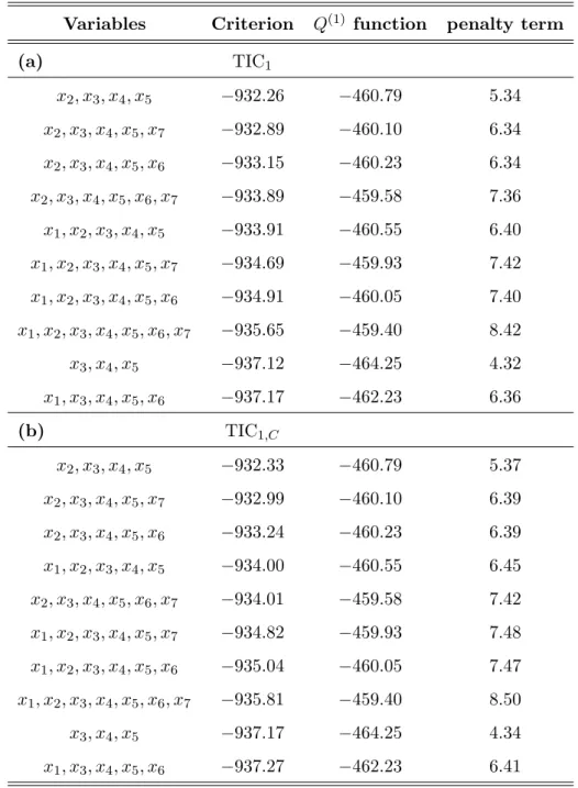
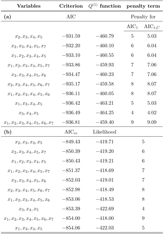
total number of all possible submodels amounts to 27 = 128. We carry out the estimation of all the possible models and we compare the results of the AIC1 and the TIC1 (both taking care of the missing observations), and the AIC for the complete cases only that ignores the missingness. Tables 2 and 3 show for each criterion the ten best models. The tables contains
the value of the criterion for each of those models, together with the Q(1) function and the penalty term. Since the models selected by AIC1 and AIC1,C happened to be the same, only
the value of AIC1 is presented. The value of AIC1,C can be computed from the given results.
The best model for all the criteria is the one that includes all the significant variables in the full model,x2, x3,x4 andx5. The three highly significant variables are always present in all the models displayed. While also the second best model is agreed upon by all criteria, the TIC1 and TIC1,C differ in their model choice from model three onwards. For model three,
the TIC1’s add variable x6, the indicator for insulin protein, while the AIC1’s add variable x1, the intraocular pressure. The difference between the TIC1 and AIC1 selected models is due to the penalty term used for calculating the criteria, since the Q(1) function is the same. Because of the large sample size, the corrected TIC1,C and the corrected AIC1,C do not give
much different results in the model selection as compared to the TIC1 and AIC1. For TIC1 and TIC1,C only the model orders of models 4 and 5 are switched. Indeed, the penalty terms
are very close for the corrected and uncorrected criteria due to the large sample size. In contrast to the simulation study, the penalty term in the TIC1 criteria is here slightly larger than the exact number of parameters.
6
Discussion
We introduced new criteria for model selection in presence of missing data, through the utilization of the EM algorithm and the weighting method of Ibrahim (1990). The new criteria are immediately obtained from the EM algorithm and can be directly compared to the AIC and TIC in case no observations are missing. We wish to stress their ease of computation and interpretation. The validity of the criteria is investigated in a simulation study and through data analysis. The results have confirmed the good performance of the criteria, in particular their efficiency to deal with the missingness. Ignoring the missing cases does not work well for model selection.
While we in this paper focussed on missing covariate data with an ignorable missingness mechanism, future work will extend these results to include missing response data and non-ignorable missingness schemes.
Table 2: Results of variable selection for the WESDR data. The table displays the best ten models selected by the different criteria, the value of the criterion for each of these models, together with the value of the Q(1) function and the penalty used for (a) TIC
1, and (b) TIC1,C. All models contain an intercept.
Variables Criterion Q(1) function penalty term
(a) TIC1 x2, x3, x4, x5 −932.26 −460.79 5.34 x2, x3, x4, x5, x7 −932.89 −460.10 6.34 x2, x3, x4, x5, x6 −933.15 −460.23 6.34 x2, x3, x4, x5, x6, x7 −933.89 −459.58 7.36 x1, x2, x3, x4, x5 −933.91 −460.55 6.40 x1, x2, x3, x4, x5, x7 −934.69 −459.93 7.42 x1, x2, x3, x4, x5, x6 −934.91 −460.05 7.40 x1, x2, x3, x4, x5, x6, x7 −935.65 −459.40 8.42 x3, x4, x5 −937.12 −464.25 4.32 x1, x3, x4, x5, x6 −937.17 −462.23 6.36 (b) TIC1,C x2, x3, x4, x5 −932.33 −460.79 5.37 x2, x3, x4, x5, x7 −932.99 −460.10 6.39 x2, x3, x4, x5, x6 −933.24 −460.23 6.39 x1, x2, x3, x4, x5 −934.00 −460.55 6.45 x2, x3, x4, x5, x6, x7 −934.01 −459.58 7.42 x1, x2, x3, x4, x5, x7 −934.82 −459.93 7.48 x1, x2, x3, x4, x5, x6 −935.04 −460.05 7.47 x1, x2, x3, x4, x5, x6, x7 −935.81 −459.40 8.50 x3, x4, x5 −937.17 −464.25 4.34 x1, x3, x4, x5, x6 −937.27 −462.23 6.41
Table 3: Results of variable selection for the WESDR data. The table displays the best ten models selected by the different criteria, the value of the criterion for each of these models, together with the Q(1) function and the penalty used for (a) AIC
1 and AIC1,C, and (b) the
complete cases only AICcc. Since the models selected by AIC1 and AIC1,C are the same, we
only show the value of AIC1. All models contain an intercept.
Variables Criterion Q(1) function penalty term
(a) AIC Penalty for
AIC1 AIC1,C x2, x3, x4, x5 −931.59 −460.79 5 5.03 x2, x3, x4, x5, x7 −932.20 −460.10 6 6.04 x1, x2, x3, x4, x5 −933.10 −460.55 6 6.04 x1, x2, x3, x4, x5, x7 −933.86 −459.93 7 7.06 x2, x3, x4, x5, x6 −934.47 −460.23 7 7.06 x2, x3, x4, x5, x6, x7 −935.17 −459.58 8 8.07 x1, x2, x3, x4, x5, x6 −936.11 −460.05 8 8.07 x1, x3, x4, x5 −936.42 −463.21 5 5.03 x3, x4, x5 −936.49 −464.25 4 4.02 x1, x2, x3, x4, x5, x6, x7 −936.81 −459.40 9 9.09 (b) AICcc Likelihood x2, x3, x4, x5 −849.43 −419.71 5 x2, x3, x4, x5, x7 −850.39 −419.20 6 x1, x2, x3, x4, x5 −850.43 −419.21 6 x1, x2, x3, x4, x5, x7 −851.37 −418.69 7 x2, x3, x4, x5, x6 −852.03 −419.01 7 x2, x3, x4, x5, x6, x7 −852.98 −418.49 8 x1, x2, x3, x4, x5, x6 −853.06 −418.53 8 x3, x4, x5 −853.39 −422.69 4 x1, x2, x3, x4, x5, x6, x7 −854.00 −418.00 9 x1, x3, x4, x5 −854.06 −422.03 5
Acknowledgements
The authors wish to express their thanks to Profs. Ibrahim and Chen for providing the Fortran code of their programs and to Dr. R. Klein for giving permission to use the WESDR data. This research is supported by the Fund for Scientific Research Flanders (G0542.06).
References
Akaike, H. (1973). Information theory and an extension of the maximum likelihood principle. In Petrov, B. and Cs´aki, F., editors, Second International Symposium on Information Theory, pages 267–281. Akad´emiai Kiad´o, Budapest.
Burnham, K. P. and Anderson, D. R. (2002). Model Selection and Multimodel Inference: A Practical Information-Theoretic Approach (2nd edition). Springer-Verlag, New York.
Cavanaugh, J. E. and Shumway, R. H. (1998). An Akaike information criterion for model selection in the presence of incomplete data. Journal of Statistical Planning and Inference, 67:45–65.
Gilks, W. R. and Wild, P. (1992). Adaptive rejction sampling for Gibbs sampling. Applied Statistics, 41:337–348.
Hens, N., Aerts, M., and Molenberghs, G. (2006). Model selection for incomplete and design-based samples. Statistics in Medicine, 25(14):2502–2520.
Hurvich, C. M. and Tsai, C.-L. (1989). Regression and time series model selection in small samples. Biometrika, 76:297–307.
Ibrahim, J. G. (1990). Incomplete data in generalized linear models. Journal of the American Statistical Association, 85:765–769.
Ibrahim, J. G., Chen, M.-H., and Lipsitz, S. R. (1999a). Monte carlo EM for missing covariates in parametric regression models. Biometrics, 55:591–596.
Ibrahim, J. G., Lipsitz, S. R., and Chen, M.-H. (1999b). Missing covariates in generalized linear models when the missing data mechanism is non-ignorable. Journal of the Royal Statistical Society, Series B, 61(1):173–190.
Klein, R., Klein, B. E. K., Moss, S. E., Davis, M. D., and DeMets, D. L. (1984). The Wisconsin epidemiologic study of diabetic retinopathy: II. Prevalence and risk of dia-betic retinopathy when age at diagnosis is less than 30 years. Archives of Ophthalmology, 102:520–526.
Kotz, S. and Nadarajah, S. (2004). Multivariate t Distributions and Their Applications. Cambridge.
Little, R. J. A. and Rubin, D. B. (2002). Statistical analysis with missing data. Wiley Series in Probability and Statistics. Wiley-Interscience [John Wiley & Sons], Hoboken, NJ, second edition.
Liu, C. (1995). Missing data imputation using the multivariate t distribution. Journal of Multivariate Analysis, 53:139–158.
Liu, C. and Rubin, D. B. (1995). ML estimation of the multivariate t distribution with unknown degrees of freedom. Statistica Sinica, 5:19–39.
Louis, T. (1982). Finding the observed information matrix when using the EM algorithm.
Journal of the Royal Statistical Society, Series B, 44:226–233.
Meng, X. L. and Rubin, D. B. (1991). Using EM to obtain asymptotic variance-covariance matrices: the SEM algorithm.Journal of the American Statistical Association, 86:899–909.
Nielsen, S. F. (2000). The stochastic EM algorithm: estimation and asymptotic results.
Bernoulli, 6(3):457–489.
Shimodaira, H. (1994). A new criterion for selecting models from partially observed data. In Cheeseman, P. and Oldford, R. W., editors, Selecting models from data: artificial intelligence and statistics IV, pages 21–29. Springer, New York.
Takeuchi, K. (1976). Distribution of informational statistics and a criterion of model fitting.
Suri-Kagaku (Mathematical Sciences), 153:12–18. In Japanese.
Appendix
Proof of Theorem 1
We use a Taylor expansion of log ˜f( ˜Y,X˜;bθ) aboutθ0 and take the expectation with respect to the true distribution of ( ˜Y,X˜) to obtain
Eg{log ˜f( ˜Y,X˜;θb)|bθ} = Eg{log ˜f( ˜Y,X˜;θ0)}+ (bθ−θ0)0Eg{ ∂ ∂θlog ˜f( ˜Y,X˜;θ0)} (9) + 1 2(bθ−θ0) 0E g{− ∂2 ∂θ∂θ0 log ˜f( ˜Y,X˜;θ0)}(θb−θ0) +op(kbθ−θ0k 2).
By definition of the least false parameter Eg{∂∂θlog ˜f( ˜Y,X˜;θ0)} = 0 and for the third
term Eg{− ∂
2
∂θ∂θ0 log ˜f( ˜Y,X˜obs;θ0)}=nI(θ0).Hence (9) reduces toEg{log ˜f( ˜Y,X˜;θb)|bθ}=
Eg{log ˜f( ˜Y,X˜;θ0)} − n2(bθ−θ0)0I(θ0)(bθ−θ0) +op(kbθ−θ0k2). After taking expectations, Kn =Eg{E˜g{log ˜f( ˜Y,X˜;θ)}}/n=Eg{logf( ˜Y,X˜;θ0)}/n−12Eg{(bθ−θ0)0I(θ0)(θb−θ0)}+ O(1/n2). The second term hereof is equal to tr{I(θ0)Var
gbθ(Y,X)}/2, where the variance
is obtained from a two-step Taylor series expansion of the first derivative of the Qfunction, which leads to,
√
n(bθ−θ0) = {−Q¨(θ0|θ0)/n}−1 1
√
nQ˙(θ0|θ0) +op(1). (10) By definition of the matricesIandJ, the trace expression simplifies to tr{J(θ0)I−1(θ0)}/(2n). This leads tonKn=Eg{logf( ˜Y,X˜;θ0)}−12tr{J(θ0)I−1(θ0)}+O(1/n).A similar Taylor se-ries expansion shows that, omitting smaller order terms that converge to zero,Kbn˙=Q(θ0|θ0)/n+
˙
Q(θ0|θ0)0(θb−θ0)/n− 12(bθ−θ0)0I(θ0)(bθ−θ0). By representation (10) and previous argu-ments, Kbn = Eg{logf( ˜Y,X˜;θ0)}/n+ 12(bθ−θ0)0I(θ0)(bθ−θ0) +rn+Op(1/n2), where rn
is an average of i.i.d. random variables with mean zero. Taking the expectation of Kbn and