SURFACE
SURFACE
Dissertations - ALL SURFACE
December 2016
Identification of key players in networks using multi-objective
Identification of key players in networks using multi-objective
optimization and its applications
optimization and its applications
R Chulaka GunasekaraSyracuse University
Follow this and additional works at: https://surface.syr.edu/etd Part of the Engineering Commons
Recommended Citation Recommended Citation
Gunasekara, R Chulaka, "Identification of key players in networks using multi-objective optimization and its applications" (2016). Dissertations - ALL. 579.
https://surface.syr.edu/etd/579
This Dissertation is brought to you for free and open access by the SURFACE at SURFACE. It has been accepted for inclusion in Dissertations - ALL by an authorized administrator of SURFACE. For more information, please contact
Identification of a set ofkey players, is of interest in many disciplines such as sociology, politics, finance, economics, etc. Although many algorithms have been proposed to identify a set of key players, each emphasizes a single objective of interest. Consequently, the prevailing deficiency of each of these methods is that, they perform well only when we consider their objective of interest as the only characteristic that the set of key players should have. But in complicated real life applications, we need a set of key players which can perform well with respect to multiple objectives of interest.
In this dissertation, a new perspective for key player identification is proposed, based on optimizing multiple objectives of interest. The proposed approach is useful in identifying both key nodes and key edges in networks. Experimental results show that the sets of key players which optimize multiple objectives perform better than the key players identified using existing algorithms, in multiple applications such as eventual influence limitation
problem,immunizationproblem, improving the fault tolerance of thesmart grid, etc. We utilize multi-objective optimization algorithms to optimize a set of objectives for a particular application. A large number of solutions are obtained when the number of objectives is high and the objectives are uncorrelated. But decision-makers usually require one or two solutions for their applications. In addition, the computational time required for multi-objective optimization increases with the number of objectives. A novel approach to obtain a subset of the Pareto optimal solutions is proposed and shown to alleviate the aforementioned problems.
As the size and the complexity of the networks increase, so does the computational effort needed to compute the network analysis measures. We show that degree centrality
based network sampling can be used to reduce the running times without compromising the quality of key nodes obtained.
USING MULTI-OBJECTIVE OPTIMIZATION AND ITS
APPLICATIONS
By
Raigamage Chulaka Gunasekara
B.Sc (Hons.) in Computer Science and Engineering, University of Moratuwa, 2009 M.Sc. in Computer Science, Syracuse University, 2015
DISSERTATION
Submitted in partial fulfillment of the requirements for the degree of Doctor of Philosophy in Computer & Information Science & Engineering
Syracuse University December 2016
There is a long list of wonderful individuals to whom I should be extremely thank-ful for helping me throughout the journey towards completing this thesis.
First and foremost, I am extremely fortunate to have two impeccable advisors; Professor Kishan Mehrotra and Professor Chilukuri K. Mohan, who have been two pillars of driving force, encouragement, and support throughout this journey. I thank my two advisors for all the fruitful research discussions, the time they were able to fit into their busy schedules when I needed, and helping to develop this study into a PhD dissertation. I am also grateful to my dissertation committee members; Professor Vir Phoha, Professor Sucheta Soundarajan, Professor Edmund Yu and Professor Utpal Roy for their time and effort in providing me with invalu-able feedback in putting together and improving my dissertation.
I should also acknowledge the former and current lab mates of the SENSE lab at Syracuse University for very fruitful weekly research meetings, their valuable feedback on my work, and for all the good times spent in Syracuse. I should also thank all my friends in Syracuse, for being a integral part of my life for the last five years.
I am also thankful for all the Professors at the Department of EECS at Syracuse University from whom I have learned invaluable new knowledge and numerous skills. I should also thank the staff members at the Department of EECS for seam-lessly handling all administrative work necessary throughout my stay at Syracuse University. I consider myself very fortunate to have had more some fantastic
thank all my teachers at Ananda College, Colombo and all my lecturers at Univer-sity of Moratuwa, Sri Lanka.
Most of all, I am grateful to my family. My wife Ishani Ratnayake; who has been selfless in supporting me every step of the way and waiting up many late nights throughout last five years. I am extremely thankful to my parents and parents in law, who have been the source of encouragement and influence throughout my life. If not for their love, support, and encouragement, none of this could have happened. I am dedicating this thesis to my precious daughter Mithuli, for being the source of unending joy and love of my life.
Acknowledgments iv
List of Tables x
List of Figures xiii
1 Introduction 1
1.1 Objectives . . . 2
1.2 Organization of the Dissertation . . . 4
1.3 Contributions . . . 6
2 Key player identification in networks 8 2.1 Key node identification in networks . . . 8
2.1.1 Degree Centrality . . . 9 2.1.2 Betweenness Centrality . . . 9 2.1.3 Closeness Centrality . . . 10 2.1.4 Eigenvector Centrality . . . 11 2.1.5 PageRank . . . 11 2.1.6 Katz Centrality . . . 12 2.1.7 HITS Score . . . 13 2.1.8 k-Core Score . . . 13
2.1.9 Identification of sets of key nodes . . . 14
2.2 Key edge identification in networks . . . 17
2.2.2 Edge betweenness . . . 18
2.2.3 Edges to improve/reduce robustness . . . 19
2.3 Concluding Remarks . . . 19
3 Decision making from multi-objective optimization 20 3.1 Evolutionary Algorithms . . . 20
3.1.1 P arent_selection . . . 22
3.1.2 Of f spring_generation . . . 22
3.1.3 Select_f or_survival . . . 24
3.1.4 Exploration vs exploitation in evolutionary algorithms . . . 24
3.2 Multi-objective optimization . . . 25
3.2.1 Evolutionary algorithms for multi-objective optimization . . . 26
3.3 Large number of solutions inO-objective optimization . . . 29
3.3.1 Selecting solutions from the Pareto optimal set . . . 29
3.4 Concluding Remarks . . . 34
4 Identifying multi-objective key nodes 35 4.1 Deficiencies of current approaches for key node identification . . . 36
4.1.1 Collective behavior of a set of key nodes . . . 37
4.1.2 Optimization of a single property . . . 40
4.2 Multi-objective optimization for identification ofkkey nodes in social net-works . . . 41
4.3 Addressing the deficiency of Eigenvector Centrality using Multi-Objective Optimization . . . 43
4.3.1 Using community information as an objective . . . 43
4.3.2 Using distance as an objective . . . 44
4.4 Selection of key players sets . . . 47
4.5 Applications of multi-objective k-key players . . . 54
4.5.1 Eventual Information Limitation problem . . . 54
4.5.2 Improving the fault tolerance of the smart grid . . . 63
4.6 Concluding Remarks . . . 78
5 Reducing the computational time 80 5.1 Network Sampling . . . 81
5.2 Degree centrality based sampling . . . 82
5.2.1 Performance of degree centrality based sampling in key node iden-tification . . . 87
5.3 Applications of multi-objective key players identified on degree centrality sample . . . 90
5.3.1 Performance of multi-objective key players in EIL problem . . . 91
5.3.2 Performance of multi-objective key player identification algorithm on the Immunization problem . . . 92
5.4 Concluding Remarks . . . 97
6 Improving network robustness using key edges 99 6.1 Robustness measures for networks . . . 100
6.1.1 Measures based on the eigenvalues of the adjacency matrix . . . 100
6.1.2 Measures based on the eigenvalues of the Laplacian matrix . . . 101
6.1.3 Measures based on other properties . . . 102
6.2 Properties of network robustness measures . . . 104
6.2.1 Analysis of trivial networks . . . 104
6.2.2 Behavior of the Robustness measures for a single edge addition to the network . . . 106
6.2.3 Correlation of robustness measures . . . 107
6.3.1 Fast calculation of robustness measures . . . 111
6.3.2 Selecting solutions from multi-objective optimization . . . 112
6.4 Experimental Results . . . 113
6.4.1 Improving robustness by edge addition . . . 113
6.4.2 Network robustness after node attacks . . . 118
6.5 Concluding Remarks . . . 120
7 Conclusions and Future work 123 7.1 Conclusions . . . 123
7.2 Future Research Directions . . . 125
4.1 Statistics of the networks used . . . 36 4.2 Collective behavior of the key players . . . 39 4.3 Set of multi-objective key players found for Dolphin Network. Objectives
: Eigenvector centrality (EC) of the super node, Number of communities represented by the key nodes . . . 44 4.4 Set of multi-objective key players found for Prisoners Network. Objectives
: Eigenvector centrality (EC) of the super node, Number of communities represented by the key nodes . . . 44 4.5 Performance Criteria and Measures for sets of Key Players . . . 51 4.6 Set of Key Players found for Dolphin Network from Pareto front and
re-spective centrality values . . . 52 4.7 Set of Key Players found for Prisoners Network from Pareto front and
re-spective centrality values . . . 52 4.8 Comparison of Pareto set pruning approaches on the number of nodes
re-cruited by the limiting campaign . . . 59 4.9 The comparison of running times (in seconds) of Pareto set pruning
ap-proaches . . . 60 4.10 Average percentage of the solutions identified by theLeave-k-outapproach
are also solutions that belong to the Pareto front of the original multi-objective optimization of the EIL problem . . . 62
tack, in the fully synthetic model . . . 75 4.12 Standard deviation of number of nodes saved after random node attacks in
the fully synthetic model . . . 75 4.13 Number of surviving nodes in the power network after a targeted node
at-tack in the fully synthetic model . . . 76 4.14 Standard deviation of number of nodes saved after targeted node attacks in
the fully synthetic model . . . 76 4.15 Number of surviving nodes in the power network after a targeted node
at-tack in the semi-synthetic model . . . 78 4.16 Standard deviation of number of nodes saved after targeted node attacks in
the semi-synthetic model . . . 78
5.1 Statistics of the largest connected component in the networks and description 81 5.2 Running times for centrality calculations in seconds (Averages over 30 runs) 81 5.3 Time taken to identify EC key players with degree centrality sampling
(sec-onds) . . . 86 5.4 Time taken to identify PR key players with degree centrality sampling
(sec-onds) . . . 86 5.5 Time taken to identify BC key players with degree centrality sampling
(sec-onds) . . . 86 5.6 Improvements of running time using Degree centrality based sampling for
multi-objective key player identification . . . 90 5.7 Average number of nodes recruited by the Limiting Campaign starting at
different delays on ca-GrQc network . . . 92 5.8 The comparison of Pareto set pruning approaches on the Immunization
problem . . . 94
ing solutions in the Pareto front of the original multi-objective optimization
(Immunization problem) . . . 95
5.10 Average Time to stabilize . . . 96
5.11 Average infection probability . . . 97
6.1 Robustness values of the trivial networks . . . 106
6.2 Correlation of the robustness measures . . . 108
6.3 Statistics and description of the networks used . . . 113
6.4 Average robustness ranks of edge addition methods; smaller values repre-sent greater robustness . . . 119
6.5 Robustness values during targeted node attacks - OpenFlights network . . . 121
6.6 Robustness values during random node attacks - OpenFlights network . . . 122
3.1 One point crossover operator . . . 23
3.2 Mutation operator . . . 23
4.1 Dolphin Network . . . 37
4.2 Creation of theSsuper as a node for a set of nodesS . . . 38
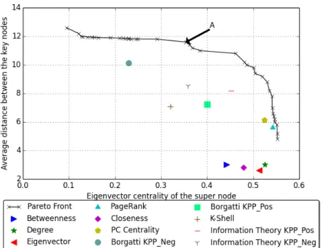
4.3 Pareto Fronts : Objectives - Eigenvector centrality of the super node and average distance between key players . . . 46
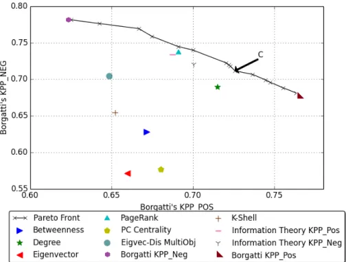
4.4 Pareto Fronts : Objectives - Borgatti’s KPP positive and negative . . . 48
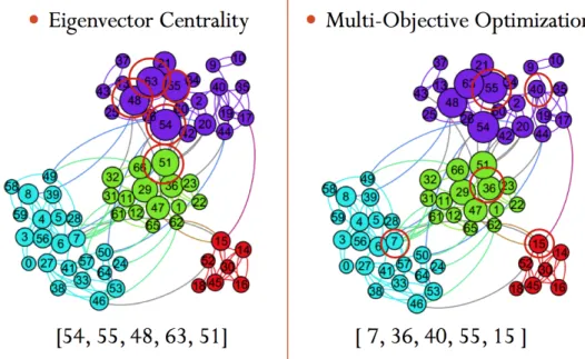
4.5 Comparison of the positions of the key players identified by the Eigenvector centrality approach vs the positions of the key players identified by multi-objective approach . . . 53
4.6 Number of nodes recruited by the Limiting Campaign starting at differnt delays . . . 64
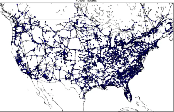
4.7 North American power grid and the degree distribution . . . 68
4.8 Cascading failures in a smart grid; the subgraph on the left (in red) shows the power network, and the network on the right (in blue) represents the communication network . . . 71
4.9 Result of cascading failures in smart grid when an extra controlling link is added to nodeC . . . 72
in retaining the original network’s top 10 key players using different cen-trality measures . . . 83 5.2 Comparison of sampling algorithms on the PGP network: performance in
retaining the original network’s top 10 key players using different centrality measures . . . 84 5.3 Pareto Fronts: Eigenvector centrality of the super node and Average
dis-tance between key players . . . 88 5.4 Pareto Fronts: Degree centrality of the super node and Betweenness
cen-trality of the super node . . . 89
6.1 Six trivial networks considered for robustness calculation; the networks are arranged in the increasing order of robustness assesed intutively. . . 105 6.2 Correlation plots between the robustness measures . . . 109 6.3 Robustness improvement in OpenFlights network - Comparison between
multi-objective approach and single objective approaches . . . 115 6.4 Robustness improvement in OpenFlights network - Comparison between
multi-objective approach and heuristic approaches . . . 117
C
HAPTER
1
I
NTRODUCTION
Networks provide an excellent platform to model many complex systems comprised of a set of entities and various relationships among them. When such a system is modeled as a network, the entities are represented as nodes (vertices), and the relationships among the entities are represented as edges. Some such systems which are commonly modeled and studied as networks include the Internet, social networks, food web, gene regulatory net-works, infrastructure netnet-works, etc. Various concepts of network theory have been used to reveal interesting patterns and open pathways to insights in the modeled systems. Starting from the well known ‘Seven Bridges of Koenigsberg’ problem in 1735, network theory has been applied to many disciplines including physics, computer science, electrical engineer-ing, biology, economics, and sociology.
Some of the interesting problems that are studied through network science include iden-tification of important entities in systems, detecting communities of users in social net-works, identifying anomalous users in social settings, modeling and analyzing information or disease spread among people in various regions, and predicting possible connections that can occur in future among people.
Modeling real-world data using networks has become popular in recent years, and the size of the networks analyzed has also grown rapidly in size. For example, social networks
such as Facebook and Twitter have reached hundreds of millions of users around the world. The World Wide Web contains at least five billion pages. As the networks grow in size, the insights that can be unveiled through network science expand, while presenting the researchers with challenges that arise with such large volumes of data.
1.1
Objectives
The main focus of this dissertation is to identify the most important entities in a system modeled as a network. These important entities are referred to askey players, throughout this dissertation. Networks consist ofnodesandedges; in this study we consider identifi-cation of both thekey nodesand thekey edges.
Key nodes in an environment represented by a network are the most important entities in the modeled environment; such as decision makers in an organization, opinion leaders in social media, celebrities and political leaders, key infrastructure nodes in an urban network, and mediators between communities.
Selecting a set of key nodes from a system that is represented as a network is an impor-tant research problem in many disciplines, such as the following:
• In viral marketing, it is important to identify and target the ‘right’ set of key people in a population to spread information efficiently and effectively.
• In human resource management, it is critical to identify and strategically place the key people to improve the productivity of the entire organization.
• In politics, it is necessary to gain the support of key individuals to gain advantages in political campaigns.
Manynode centralitymeasures have been proposed to capture the different behaviors a node can have in a social setting. These node centrality measures are used to identify key nodes in a networks, and are discussed in Chapter 2.
Identifying the important edges in a network plays an important role in applications such as the following:
• In information diffusion applications, it is important to identify the edges which play an important role in diffusing information more efficiently among different parts
(communities)in the network.
• In determining and strengthening robustness of networked environments, it is impor-tant to identify the connections that upon removal would collapse the network, and take necessary measures to protect these connections from attacks and failure.
Current approaches proposed to identify key edges include methods based on the strength of the edges, edge centrality measures and optimization techniques addressing a specific property of interest to the network. These measures are discussed in Chapter 2 and Chapter 6.
One common property of all the current approaches for key player identification is that each of these methods identifies key players based on a single characteristic of interest. For example, one trivial method to identify important nodes in a network is to count the number of edges incident on each node. Intuitively, an important node in a network should be con-nected to more peers in a network setting. But, this method of key node identification does not consider the structure of the network and the positions to which these selected nodes belong in the network. Hence, the identified key players might come from the periphery of the network, which may not correspond to the most important positions in a network.
We investigate the effects of using key players which optimize multiple properties of interest in different well known applications of network science. Our hypothesis is that when a set of key players optimizes multiple properties which are relevant for a particular application, this set of key players should outperform the sets of key players identified based on a single property of interest. Towards this goal, we identify bothkey nodes and
that key players which optimize multiple objectives perform better than the key players identified using existing algorithms.
We utilize multi-objective optimization algorithms (such as NSGA-II) to optimize a set of objectives for a particular application. Such an approach identifies a set of solu-tions (rather than one solution needed by a typical decision-maker), which are ‘equally’ good in optimizing the set of objectives. In addition, the computational time required for multi-objective optimization increases with the number of objectives. To alleviate these problems, we propose a technique which approximates the solutions in the multi-objective optimization. The proposed approach utilizes a two-step process to multi-objective opti-mization, and has advantages such as: (1) reducing the number of solutions in the solution space, (2) reducing the computational time significantly, and (3) providing solutions which deliver performance ‘similar’ to the performance obtained by the solutions given by the unmodified multi-objective optimization algorithm.
As the size and the complexity of the networks increase, so do the computational times associated with the network analysis measures. Hence, we focus on how network sampling can be used to reduce the running times without compromising much on the quality of key nodes obtained. We introduce the idea ofdegree centrality based sampling to reduce the running time of the key node identification problem. We show that the multi-objective key player sets obtained with degree centrality based sampled networks perform better than single objective key player sets identified by applying the algorithms on the entire network.
1.2
Organization of the Dissertation
This dissertation is organized as follows. In Chapter 2, we discuss the related work on key node and key edge identification methods. We discuss the widely used centrality measures, and optimization techniques proposed to identify key players in networks.
the background of multi-objective optimization tasks, and discuss how evolutionary algo-rithms have been used to solve multi-objective optimization. One prevailing issue with multi-objective optimization is that it identifies a set of solutions, rather than a single so-lution as required by most decision makers. In addition to that, the time complexity of multi-objective optimization increases with the number of objectives. To alleviate these is-sues, we propose theleave-k-outapproach for multi-objective optimization. We show that the solutions for multi-objective optimization obtained using our approach perform well compared to other approaches proposed to select solutions from a set of solutions obtained by multi-objective optimization, while reducing the computational time significantly.
In Chapter 4, we propose the algorithm for identifying key nodes which optimize mul-tiple objectives of interest. In our approach we transform the network of interest into a bit string, and applyleave-k-outapproach for multi-objective optimization to obtain key nodes which optimize multiple properties of interest. We show that by using this approach we can alleviate some of the prevailing problems of key node identification. Then we compare the different key node identification methods in two well known applications, viz., Even-tual Information Limitation (EIL)and improving the fault tolerance of thesmart grid, and show that the multi-objective approach outperforms the previous key node identification methods.
As the size and the complexity of the networks increase, so do the running times of the network analysis measures. The proposed multi-objective approach to key player identifi-cation depends on the computational complexity of individual network centrality measures and on the computational complexity of evolutionary optimization algorithm employed. The focus of Chapter 5 is on how network sampling can be used to reduce the running times of key player identification without compromising much on the quality of key nodes obtained. First, we give an overview of the common network sampling methods. Next, we propose the idea of degree centrality based sampling approach to reduce the running time of the key node identification problem. Finally, the multi-objective key player sets
obtained on degree centrality based sampled networks are used to address two well known problems, viz.,Eventual Information Limitation (EIL)problem andImmunizationproblem. The results suggest that the multi-objective key player sets identified on sampled networks perform better than single objective key player sets identified by applying the algorithms on the entire network.
In Chapter 6 we address key edge identification. When edges are added to a network, the properties of the network change. The amount of change depends on the importance of the set of edges that are added to the network. In this study, we assume that upon addi-tion a set of key edgesshould maximally improve the network robustness. In this chapter we address the following problem : Given a network and a budget, how should a set of ‘key’ edges be selected to be added to the network in order to maximally improve the over-all robustness of the network. Towards this goal, first we discuss the network robustness measures that have been proposed and widely used. Then, we analyze the properties of these robustness measures and identify their similarities and dissimilarities using correla-tion analysis. Then, we use multi-objective optimizacorrela-tion and theleave-k-out approach to optimize multiple robustness measures of interest to improve the overall robustness of a network. We provide experimental evidence which shows the improvement in multiple robustness measures when the new edges are added using our algorithm.
Finally, Chapter 7 provides the concluding remarks of this study and the future direc-tions of research.
1.3
Contributions
The main contributions of this thesis are as follows.
1. We are the first to propose an approach that identifies a set of key nodes which op-timize multiple properties of interest. The experimental results show that the key nodes identified using this approach outperform the key nodes identified using other
approaches in multiple well known applications.
2. A key edge identification method, which optimize multiple properties of interest is proposed. The sets of key edges identified using this approach improves the overall robustness a network, compared to previous approaches to key edge identification.
3. We propose a two-step approximation approach for multi-objective optimization. The solutions obtained for multi-objective optimization using our approach perform ‘equally’ well compared to other approaches proposed to select solutions from a set of solutions obtained by multi-objective optimization, while reducing the computa-tional time significantly.
4. A sampling approach based ondegree centralityis proposed. We show that on mul-tiple applications, the multi-objective key player sets identified on sampled networks perform better than the single objective key player sets identified by applying the algorithms on the entire network.
C
HAPTER
2
K
EY PLAYER IDENTIFICATION IN
NETWORKS
As discussed in Chapter 1, key player identification in networks is an important problem. Hence, over the years many algorithms have been proposed to solve this problem. This chapter summarizes previous work on key player identification in networks, considering key node identification as well as key edge identification.
2.1
Key node identification in networks
Given a networkG= (V, E)with a set of nodesV and a set of edgesE ⊆V ×V , network centrality measures assign a value to the nodes inV based on the structural properties of the network. The score each node gets assigned depends on the property of interest. A network centrality measure is a function that maps a nodev in the networkG= (V, E)to a real number. Based on the value each node receives from the centrality measure, a rank can be assigned to each node. This rank determines the importance of a node with respect to the structural property on which the centrality measure is based. In this section, some of the most widely used centrality measures are presented.
2.1.1
Degree Centrality
The number of vertices adjacent to a given vertex in a network is the degree of that vertex.
Degree centrality is defined as the ratio of the number of neighbors of a vertex with the total number of neighbors possible [75].
Cdegree(x) =d(x) (2.1)
Cdegree centrality(x) =
d(x)
(n−1) (2.2)
where,d(x)is the number of nodes adjacent to nodex, andnis the total number of nodes in the network. For networks with directional edges (directed networks), two variants of node degree are defined. In directed networks, the In-degree of a vertex x refers to the number of edges received by x, and theOut-degree of a vertexx refers to the number of edges initiated by x. Degree centrality is used to rank vertices in a network based on the number of direct connections of each vertex, where the implication is that the vertices that have more direct connections are more important. Degree centrality is a local measure and does not consider the importance of the vertices to whom each vertex is connected; hence using degree centrality to identify key nodes may not be satisfactory in some cases.
2.1.2
Betweenness Centrality
The degree of a node is not the only measure of the importance of a node in a network. In
Betweenness centrality, the nodes which have a high probability of occurring in shortest paths of other nodes are considered to be more important [45, 81].
Cbetweenness centrality(x) = X y,z6=x, σy,z6=0 σy,z(x) σy,z (2.3)
where,σy,zis the number of shortest paths between nodesyandz, andσy,z(x)is the number
centrality often act as bridges between different communities in a network. Thus, removal of a node with high betweenness centrality can lead to increase in the geodesic path lengths, and in the extreme case, the network might even get disconnected. In real world networks, this can be important; for example, to prevent the spread of a disease in an epidemic net-work. A common criticism for shortest-paths based measures is that they do not take into account spread along non-shortest paths. Hence, betweenness measures that relax this as-sumption by including contributions from essentially all paths between nodes (not just the shortest) have also been proposed [83].
2.1.3
Closeness Centrality
Incloseness centrality, the nodes with smallest paths to other nodes are considered more important, formally defined as the length of the average shortest path between a vertexx and all other vertices in the network [92].
Ccloseness centrality(x) = n X j=1 d(x, i) (n−1) −1 (2.4)
whered(x, i)is the shortest path distance between nodesxandi, andnis the total number of nodes in the network. This can be used to measure how long it will take to spread information from nodexto all other nodes, and thus plays an important role in information propagation in networks. For disconnected networks, Harmonic Centrality, which is a variant of closeness centrality, has been defined as follows:
Charmonic centrality(x) = X
x6=i
1
d(x, i) (2.5)
2.1.4
Eigenvector Centrality
Eigenvector centralityassigns relative scores to all nodes in the network based on the con-cept that connections to high-scoring nodes contribute more to the score of the node of interest [13]. Unlike degree centrality, in this case the importance of the neighbors is also taken into account.
The eigenvector centralities of all the nodes in the network (vectorx) are defined using the equation,
Ax=λ1x (2.6)
whereAis the adjacency matrix of the network andλ1is the highest eigenvalue ofA.
The power iteration method is used to approximate eigenvector centrality. Here, the eigenvector centrality of a vertex is iteratively recomputed as the sum of centralities of its neighbors. To begin the power iteration method, it is assumed that vertexihas eigenvec-tor centrality ofxi(0). Then we gradually improve this estimate by employing a Markov
model, and continue until no more improvement is observed. The estimate made at stept is defined as, xi(t) = X j Aijxj(t−1) (2.7) i.e., x(t) = Ax(t−1) and, x(t) =Atx(0) (2.8)
2.1.5
PageRank
PageRank is a link analysis algorithm used by the Google Internet search engine, that assigns a numerical weighting to each element of a hyperlinked set of documents, such
as the World Wide Web [94]. The PageRank of a page is defined recursively and depends on the PageRank metric of all pages that link to it. A page that is linked by many pages with high PageRank receives a high rank. The same concept applies to identifying nodes with high PageRank in a network. PageRank can be thought of as approximately a probability distribution representing the likelihood that a random walk in the network will arrive at any particular node. P R(i) = 1−β n +β X (j,i)∈E P R(j) L(j) (2.9)
where n is the number of nodes in the network, β is the damping factor defined for the network.
2.1.6
Katz Centrality
In Katz centrality a weighted count of all nodes that are connected to a certain node is considered. The weight of a path of lengthdis computed with attenuation factorβd, where βis the attenuation constant defined for the application [65].
ki =Iij +β X j Aij +β2 X j A2ij +β3X j A3ij +... or, in vector notation,
k = (I+βA+β2A2+β3A3+...)e k = ∞ X i=0 (βiAi)e k= (1−βA)−1e (1−βA)k =e (2.10)
2.1.7
HITS Score
Hyperlink-Induced Topic Search (HITS) (hubs andauthorities) is another algorithm that can be used to rank nodes in a network. In the world wide web, a good hub represents a page that points to many other informative pages, and a good authority represents a page that is linked by many different hubs [69].
The algorithm assigns two scores for each page: its authority value, which estimates the value of the content of the page, and its hub value, which estimates the value of its links to other pages. The authority centrality of a node i(xi) is proportional to the sum of hub
centralities of nodes (yj) pointing to it, and is defined as
xi =α X
j
Ajiyj (2.11)
The hub centrality of a node is proportional to the sum of authority centralities of nodes it points to, and is defined as
yi =β X
j
Aijxj (2.12)
2.1.8
k-Core Score
k-Core score is another recent approach to identify key nodes in a network. The argument for this approach is that the best spreaders in the network reside in the core of the network [68], and are identified by k-shell decomposition. The process assigns an integer index or coreness,kxto each node, representing its location according toksuccessive layers (shells)
in the network. Small values ofksdefine the periphery of the network and the innermost
network core corresponds to largeks.
The process of assigningksvalues for each node is as follows.
i. Start by removing all nodes with degreek = 1.
continue pruning the network iteratively until there is no node left with k = 1 in the network.
iii. The removed nodes, along with the corresponding links, form a k shell with index ks = 1.
iv. In a similar fashion, iteratively remove the next shell,ks = 2, and continue removing
higher-k shells until all nodes are removed.
2.1.9
Identification of sets of key nodes
In some cases it is necessary to identify a set of key nodes, rather than one important node for the whole network. Some of the examples of such cases involve the following:
1. A network comprised of several communities, so the key nodes should ideally come from different parts of the network.
2. A set of key nodes with multiple capabilities are needed to be identified.
The problem of identifying an optimal set of k players is different from the problem of selecting k individuals that are each individually optimal. Ideally, an algorithm that identifies a set of key nodes should identify k key nodes that can ‘collectively’ perform well. A few methods have been proposed to find sets of key nodes capable of optimizing some performance criterion.
Group centrality
The concept of centrality has been applied not only to single individuals within a network but also to groups of individuals, for example, measures for degree centrality, closeness and betweenness are defined for a group [39]. Using these measures, a group having high centrality will be the key node set. It must be remarked that group centrality can be used
not only to measure how ‘central’ or important a group is, but also in constructing groups with maximum centrality within an organization.
Combinatorial optimization to identify key node sets
Borgatti [14] described how to find a set of key nodes considering two different aspects. He defined the set of nodes maximally connected to all other nodes asKPP-Posand the set of nodes whose removal would result in a residual network with the least possible cohesion asKPP-Neg.
i. KPP-POS - These are the key nodes for the purpose of optimally diffusing something through the network by using the key nodes as seeds. A measure for identifying the measure of reach (DR), for a set ofkkey nodes was defined as follows.
DR= X j 1 dK(j) n (2.13)
where,dK(j), is the minimum distance from any member of set of nodesK to nodej,
andnis the total number of nodes in the network. The set ofknodes which gives the highestDRis considered to be thekkey nodes for KPP-POS.
ii. KPP-NEG - These are the key nodes for the purpose of disrupting or fragmenting the network by removing the key nodes. A measure of Fragmentation(DF), for a set ofk
key nodes was defined as follows.
DF = 1− 2X i>j 1 dij n(n−1) (2.14)
where,dij, is the minimum distance between nodesiandj, andnis the total number
of nodes in the network. The set of k nodes, whose removal gives the highest DF
To identify the best set of nodes for each of the above problems, the following proce-dure (combinatorial optimization) is followed.
Algorithm 1: Greedy Combinatorial optimization
1: Selectknodes at random to populate setS
2: FindF = fitness value for the setSusing appropriate key node metric
3: forNodeu∈S do
4: forNodev 6∈Sdo
5: ∆f = improvement in fitness ifuandvwere swapped
6: end for
7: end for
8: if∆f≤0then
9: Terminate
10: else
11: Swapuandv with greatest∆f and setF =F + ∆f
12: Go to step 3
13: end if
Information Theory to identify key node sets
Ortiz-Arroyo and Hussain [93] proposed an Information Theory based measure to find
KPP-Pos and KPP-Negkey node sets. This method relies on the structural properties of the network, and uses Shannon’s definition of entropy to define the measures.
The connectivity probability distribution of the network is defined as,
χ(vi) =
deg(vi)
2n
Using the above definition, the connectivity entropyHco, is defined as follows,
Hco(G) = − n X
i=1
χ(vi)×log2χ(vi) (2.15)
The connectivity entropy measure provides information about the connectivity degree of a node in the graph.
geodesic paths that have nodevi as source and the rest of nodes in the network as targets.
This is called the centrality probability distribution.
γ(vi) =
paths(vi) paths(v1, v2, .., vM)
wherepaths(vi)is the number of shortest paths from nodevi to all the other nodes in the
network andpaths(v1, v2, ..., vM)is the total number of shortest pathsM that exists across
all the nodes in the graph. Using the above definition, the centrality entropyHce, is defined
as follows, Hce(G) =− n X i=1 γ(vi)×log2γ(vi) (2.16)
Centrality entropy provides information on the degree of reachability for a node in the graph. The algorithm in [93] attempts to solve KPP-POS and KPP-NEG problems using connectivity entropy and centrality entropy. To solve the KPP-POS problem, the set of nodes that produce the largest change inHcois selected. To solve the KPP-NEG problem,
the set of nodes that produce the largest change inHceis selected.
2.2
Key edge identification in networks
Typically, key players in networks refer to important nodes in the network. However in some contexts such as network robustness, edges also play an important role. Although many approaches in the literature have been proposed to identify important nodes, there are very few studies on identifying key edges in networks. Identifying the important edges in a network plays an important role in applications such as the following:
• In information diffusion applications, it is important to identify the edges which play an important role in diffusing information more efficiently among different parts (communities) in the network.
impor-tant to identify the edges that upon removal would collapse the network, and take necessary measures to protect these edges from attacks and failure.
As mentioned earlier, the number of methods proposed in literature to identify key edges are limited compared to the number of methods proposed in identifying key nodes in networks. In this section, some of the previous work on key edge identification is summa-rized.
2.2.1
Edge weights
Most of the networks that have been studied are binary in nature; that is, the edges be-tween vertices are either present or not. But some of the networks can also be weighted, meaning their edges can have differing strengths; there may be stronger or weaker social ties between individuals. For example, in a network representing the email exchanges in an office environment, the number of email messages exchanged between two persons can be considered as the edge weight between the corresponding nodes.
As the edges with the highest weights represent the most frequent interactions in the network, edge weights provide a useful means to identify important edges in a weighted network [36].
2.2.2
Edge betweenness
Node betweenness has been studied in the past as a measure of importance of nodes in networks [45, 81]. In order to identify the important edges in a network in terms of ap-pearing in ‘between’ the shortest paths of pairs of vertices, the node betweenness centrality has been generalized to edges [48]. According to the notation introduced in [48], the edge betweenness centrality for the edgeeis defined as,
Cedge betweenness(e) = X x6=y∈V σx,y(e) σx,y (2.17)
where, σx,y(e) is the number of shortest paths between the nodes x and y, that includes
edge e, and σx,y is the total number of shortest paths between the nodes x and y. This
measure reflects the total number of shortest paths between nodes in the network that rely on a given link. Thus, edges with higher edge betweenness centrality are generally more important for maintaining the connectivity of the network than edges with low centrality.
2.2.3
Edges to improve/reduce robustness
When edges are removed from a social network, the properties of the network change. This amount of change depends on the importance of the set of edges that gets removed. The set ofk edges that can reduce the robustness the most upon removal or the set ofk edges upon addition that can increase the robustness the most can be considered as ‘key’ edges in a network. For example, in [21] the set of edges that minimize the natural connectivity of the network [63] upon removal, and the set of edges that maximize natural connectivity upon addition were identified as the important edges in the network. These methods are discussed in detail in Chapter 6, where we focus on improving the network robustness using key edges.
2.3
Concluding Remarks
In this chapter we reviewed some of the previously proposed approaches for key node and key edge identification in network. One underlying property of all the approaches discussed in this chapter is that each of them focuses on one property of interest. But in complicated real life applications, we need a set of key players that can perform well with respect to multiple objectives of interest. To address this problem, in chapter 4, we propose a new algorithm for identifying key players which optimizes multiple objectives of interest.
C
HAPTER
3
D
ECISION MAKING FROM
MULTI
-
OBJECTIVE OPTIMIZATION
This chapter introduces evolutionary algorithms and multi-objective optimization, discusses on problems of using multi-objective optimization to real-world decision making. This chapter is organized as follows. Section 3.1 gives an overview of Evolutionary Algorithms (EAs). In Second 3.2, we formally describe the problem of multi-objective optimization. Section 3.3 discusses the problem that multi-objective optimization algorithms produce too many solutions when the number of objectives are high and conflicting, and discusses the approached proposed to solve this problem.
3.1
Evolutionary Algorithms
Various techniques have been proposed to solve optimization problems, and these tech-niques can be classified into three categories: exhaustive, deterministic and stochastic.
Inexhaustive search, the entire decision space is searched in order to find the optimal solution. Therefore, exhaustive search techniques are highly computationally expensive and cannot be applied to real world large problems. Deterministic searchmethods
incor-porate domain knowledge to reduce the size of the search space, which is subsequently probed through tree like or graph like walks. Although the domain knowledge helps to reduce the search space and computational complexity, the domain knowledge is not al-ways available to reduce the search spaces of interest. Evolutionary Algorithms belong to the third category; stochastic search, and work by repeatedly sampling the search space, guided by the information collected during the search process. Compared to other methods, Evolutionary Algorithms typically do not attempt to search the entire decision space, and are not guaranteed to find the optimal solution.
Inspired by the natural evolution process [43, 22], Evolutionary Algorithms iteratively modify a population of candidate solutions for the optimization problem. Each solution in the optimization process is referred to as an individual, and through repeated application of randomized processes of recombination, mutation and selection, the individuals are altered until specified termination criteria are met. A typical Evolutionary Algorithm is described by the pseudo-code shown in Algorithm 2 [34].
Algorithm 2: A typical evolutionary algorithm
1: i←0
2: P(i)←Random set of individuals (initial population)
3: Evaluate the fitness of all individuals ofP(i)
4: Choose a maximum number of generationsimax
5: whilei < imax do
6: i=i+ 1
7: M(i) = P arent_selection(P(i−1))
8: C(i) = Of f spring_generation(M(i))
9: P(i) =Select_f or_survival(P(i−1), C(i))
10: Evaluate the fitness of all individuals ofP(i)
11: end while
12: Return the best individual ofP(i)
Evolutionary Algorithms begin with generating an initial population of individuals drawn at random from the decision space. Then, at each generation i, the mating pool M(i)is generated from the population currently stored asP(i−1).
3.1.1
P arent
_
selection
During the P arent_selectionstage, an objective function is used to compute the fitness value of each candidate solution, which indicates the quality of the solution. A selection mechanism is then used to select individuals to be used as parents to those of the next generation. Individuals with a high fitness value are given a higher probability to be placed into the mating pool for reproductive purposes. Roulette Wheel Selection[49], Stochastic Universal Sampling[4], Tournament Selection[9] and Truncation Selection[85] are a few of the most common selection techniques used in literature.
3.1.2
Of f spring
_
generation
During the this step, genetic materials between the selected parents are exchanged within the mating pool and it results in the creation of the child populationC(i). Offspring gen-eration usually occurs in two forms: crossover and mutation. Every offspring gengen-eration operation has an associated probability of occurrence, which is a parameter usually prede-termined and kept unchanged throughout the search process.
Crossover or Recombination
The crossover operator is applied to two individuals in the parent population. This creates two new offspring individuals each having different subsets of the alleles of the parents. Figure 3.1 gives an example for one point crossover; a commonly used variant of crossover operator. Here, the point of crossover is determined to be at a particular point, and then the first child inherits alleles (bits) of the first parent upto the crossover point and the alleles of the second parent after the crossover point. The second child inherits alleles of the second parent upto the crossover point and the alleles of the second parent after the crossover point. Other crossover operators have also been proposed in the literature, e.g., two-point crossover and uniform crossover. The new chromosome may be better than both of the
parents if it takes the best characteristics from each of the parents.
Fig. 3.1: One point crossover operator
Mutation
A mutation operator modifies an individual in the parent population by a slight alteration. Usually this is done by flipping one or more bits of an individual in the parent population to create a new child. Figure 3.2 gives an example of the mutation operator where one bit (5thbit) is flipped to create a new child. Mutation allows the development of un-inherited
characteristics in individuals and promotes diversity by allowing an offspring to evolve in ways not solely determined by traits inherited by parents.
3.1.3
Select
_
f or
_
survival
In this stage, the fitness values of the individuals of the current populationP(i−1)and the child populationC(i)are compared, and the individuals that form the next generation of the population P(i) are identified. The selection of individuals in this stage does not completely depend on the fitness values.Elitisminvolves using a small fraction of the fittest candidates in the parent population(P(i−1))in the new population(P(i))unaltered, even though fitness values of some of these individuals are less than that of the individuals found after recombination in(C(i))[32]. Elitism avoids the risk of losing highly fit individuals from later generations.
3.1.4
Exploration vs exploitation in evolutionary algorithms
The balance between theexplorationof unexamined regions of the search space and the ex-ploitationof regions already identified as areas containing good solutions plays an impor-tant role in evolutionary algorithms [29]. This can be adjusted by modifying the selection pressure implemented using the selection operator and the probability of mutation.With selection pressure, more emphasis is given to selecting the individuals with high fitness. A strong selection pressure may cause the algorithm to converge rapidly to a local optimum, and a low selection pressure may cause the algorithm to yield random results that differ from one run to another. Crowding[30] is one of the techniques that is widely used to preserve diversity under selection pressure in evolutionary algorithms [79]. There are two main steps involved in crowding. In the pairing step, the offspring individuals are paired with individuals in the parent population according to a similarity metric. In the replacement step, a decision is made for each pair of individuals as to which of them will remain in the population.
Mutation is used to enhance exploration, flipping random bits in an individual. A very high mutation rate increases the probability of searching more areas in search space, pre-venting the population from converging to optimum solution. On the other hand, a very
low mutation rate may result in premature convergence. Hence, the selection of the proper mutation rate for the application at hand is important in determining the performance of the evolutionary algorithm.
3.2
Multi-objective optimization
Multi-objective optimization is the process of optimizing (minimizing or maximizing) a number of objectives simultaneously. A multi-objective optimization problem may also contain a set of constraints which any feasible solution must satisfy. In general, a multi-objective optimization problem can be defined as follows:
Find the vectorx∗ that optimizes a given set ofOobjective functions, i.e.,
M aximize/M inimize F(x∗) = [F1(x∗), F2(x∗), ..., FO(x∗)]T
subjected to the constraints,
gj(x∗)≤0 ;j = 1,2, ..., k hl(x∗) = 0 ;l = 1,2, ..., e
Each objective functionFi(x)must be maximized or minimized,Ois the number of
ob-jective functions,kis the number of inequality constraints, andeis the number of equality constraints.
In many real-life problems, various objectives conflict with each other. Hence, opti-mizing with respect to a single objective results in poor solutions with respect to the other objectives. Therefore, in multi-objective optimization we obtain a set of solutions, each of which satisfies the objectives at an acceptable level without being dominated by any other solution.
solutions, each of which is non-dominated by any other solution. A solution X is non-dominated, if every solution better thanX with respect to one objective function, must be worse than X with respect to another objective function. For example, in a car purchase problem scenario, two objectives of interest to a buyer would be the cost and the engine performance. Alternatives may include a car which has low cost and low engine perfor-mance, and another car which comes with high cost and high engine performance. In this scenario, neither is strictly ‘better’ than the other according to both cost and performance criteria. Such solutions are called Pareto optimal solutions. The set of all possible non-dominated solutions in X is called the Pareto optimal set. The corresponding objective function values of the Pareto optimal set in the objective space constitute thePareto front. The goal of a multi-objective optimization algorithm is to identify solutions in the Pareto optimal set.
3.2.1
Evolutionary algorithms for multi-objective optimization
Many different methods exist to solve multi-objective optimization problems. The most common technique is to aggregate the multiple objectives into a single objective by using weighted sum model [86]. Another trivial technique is to optimize the objectives one at the time, with a given order of importance of the objective functions [86]. However, finding the appropriate weight assignment for the objective functions is generally non trivial and problem-dependent. In additions, since these techniques arbitrarily limit the search space some Pareto optimal solutions will not be considered [26].The application of evolutionary algorithms to solve multi-objective optimization prob-lems is similar to Algorithm 2. However, multi-objective optimization algorithms should also consider how the fitness values should be assigned to individuals to lead the evolution to a Pareto optimal set and how to maintain diversity in the population to avoid premature convergence [34].
algo-rithm proposed to solve multi-objective optimization. During each generation of VEGA, a number of sub-populations are generated by performing proportional selection according to each objective function. Then these sub-populations are shuffled, and regular GA op-erations are carried out on the shuffled populations. The concept of Pareto optimality was introduced by David E. Goldberg in [50], and has been used by almost all the evolutionary algorithms proposed to solve multi-objective optimization afterwords.
Non-dominated Sorting Genetic Algorithm (NSGA) was proposed by Srinivas and Deb [106], and is based on several layers of classification of the individuals. The key steps of the NSGA are as follows:
i. Before selection, the population is ranked based on domination, where all non-dominated individuals are given the same rank.
ii. All these individuals share the same fitness value.
iii. Then, this group of individuals are ignored and the next set of non-dominated individ-uals are obtained from the remaining layers.
iv. These individuals are given a fitness value less than that of the previous set.
v. The process continues until all individuals in the population are assigned a rank.
Since the individuals in the first non-dominating set have the highest fitness value, more individuals of that set get selected to the mating pool. NSGA was shown to be a computa-tionally expensive algorithm for multi-objective optimization because of repeated calcula-tion of non-dominating sets [27]. Niched-Pareto Genetic Algorithm (NPGA) [56], which uses a tournament selection scheme based on Pareto dominance, and Multi-Objective Ge-netic Algorithm (MOGA)[44], which ranks individuals based on the number of other indi-viduals which are dominated by it, were also proposed during the same period. Strength Pareto Evolutionary Algorithm (SPEA) [127] uses a generational gap elitist approach,
Algorithm 3: The NSGA-II algorithm
1: i←0
2: Pi ←Random set of individuals (initial population) of sizeN
3: Evaluate the fitness of all individuals ofPi
4: Apply crossover and mutation toPito create offspring populationCiof sizeN
5: Choose a maximum number of generationsimax
6: whilei < imax do
7: SetRi =Pi∪Ci
8: Identify the non-dominated frontsF1, F2, ..., FkinRi.
9: forj = 1, ...kdo
10: Calculatecrowding distanceof the solutions inFi
11: Pi+1 =∅ 12: if(|Pi+1|+ Fj ≤N)then 13: Pi+1 =Pi+1∪Fj 14: else
15: Add the least crowdedN −|Pi+1|individuals fromFj toPi+1
16: end if
17: end for
18: Use binary tournament selection based on the crowding distance to select parents fromPi+1
19: Apply crossover and mutation toPi+1to create offspring populationCi+1of size N 20: i←i+ 1
21: end while
where a proportion of the current population is preserved and carried to the next gener-ation. Strength Pareto Evolutionary Algorithm 2 (SPEA2) [126] is an improved version of the SPEA.
The most widely used evolutionary algorithm for multi-objective optimization is the Non-dominated Sorting Genetic Algorithm-II (NSGA-II) [31], which is an improved ver-sion of NSGA [106], and is shown in Algorithm 3.
NSGA-II estimates the density of solutions surrounding a particular solution in the population by computing the average distance of two points on either side of this point along each of the objectives of the problem. This value is called thecrowding distance. During selection, the NSGA-II considers both the non-domination rank of an individual and its crowding distance. The elitist mechanism used in NSGA-II consists of combining the best parents with the best offspring obtained. NSGA-II is much more efficient than its
predecessor, and the superior performance is evident from the wide usage of the algorithm in wide range of applications [70].
Some of the more recent evolutionary algorithms proposed to solve multi-objective optimization problems includes MOEA/D [125], BORG[53] and NSGA-III [33, 61].
As NSGA-II has been widely used and shown superior performance in multiple appli-cations, we use NSGA-II as the multi-objective optimization algorithm in this study.
3.3
Large number of solutions in
O
-objective
optimiza-tion
One issue with regard toO-objective optimization is that we obtain a large number of so-lutions when the value ofOis high and the objectives are uncorrelated [46, 41, 7]. But, the decision makers who use multi-objective optimization in their applications usually require one or two solutions to be used in their applications. Multiple methods have been proposed in literature to prune the Pareto optimal set of solutions. This section discusses some of the methods proposed in literature.
3.3.1
Selecting solutions from the Pareto optimal set
The methods proposed to select solutions from the Pareto optimal set can be divided into three categories.
Ranking methods
In ranking methods, after executing the multi-objective optimization algorithm, the set of Pareto optimal solutions obtained are ranked according to a user-specified certain criteria. Once the ranking is done, the decision maker can pick the solutions that are best ranked for the desired applications. Some of the proposed ranking methods include the following:
1. Weighted sum approach (WS):
This is the most widely used approach for pruning solutions from the Pareto optimal set. For anO-objective optimization problem, the weighted sum rank of the Pareto optimal solutionXi is given by,
W S(Xi) =
O
X
j=1
wjOj(Xi), (3.1)
wherewj is the weight assigned to the objectiveOj. The weight assignment to the
objectives is domain dependent and the decision maker should determine the appro-priate weight assignment to the objectives. The result of the ranking depends on the weight assignment. Hence, in applications where the proper weight assignment is unknown, the results of the weighted sum approach are questionable [46].
2. Average Ranking (AR):
This method uses the average of the ranking positions of a solution Xi given by all
the objective functions, and is calculated as follows:
AR(Xi) = O X j=1 Rj(Xi) O , (3.2)
whereRj(Xi)is the rank given to the solutionXi by the objectiveOj.
3. Maximum Rank (MR):
This approach does not assign a rank to each of the solutions in Pareto set. The main steps of the MR are as follows,
i. Solutions in the Pareto set are ranked separately for each objective. ii. The best rankedkpoints from each objective are extracted.
to extract solutions from extreme points in the Pareto surface [120].
Pruning methods
The solution pruning methods proposed in the literature can be divided into two categories.
1. Clustering:
The clustering method assumes that the output of the pruning process should be the distinct solutions in the objective space. The number of clusters can either be determined by the decision maker or can be optimized according to the Pareto set solutions. For each cluster, one representative solution is chosen in which often the solution nearest to the center of the cluster is used. The number of clusters is optimized using the average silhouette width [98]. For a solution Xi, this approach
calculates the average distancea(Xi)to all other points in its cluster and the average
distanceb(Xi)to all other points in the nearest neighbor cluster.
Silhouette(Xi) =
b(Xi)−a(Xi) max(ai, bi)
(3.3)
A silhouette value close to1indicates that the solution was assigned to an appropri-ate cluster. If the silhouette value is close to0, it means that the solution could be assigned to another cluster; and if it is close to−1, the solution is considered to be misclassified. The overall silhouette width is the average of the silhouette values of all solutions. The largest silhouette width indicates the best clustering and therefore the number of clusters associated with this best clustering is taken as the optimal number of clusters. The following are two approaches used to select representative points from the clusters.
(a) Cluster centers (CC):
clusters are chosen as the representative points from each cluster. In [23], k-means [54] is used as the clustering algorithm, and the cluster centroids are picked as the representative points.
(b) Points closest to the Ideal point (IP):
The main steps of this approach are as follows [24].
i. For each cluster, the ideal point is identified. The ideal point of a subset of points is the virtual point that has a minimal evaluation for each objective. ii. Then, for each point in each cluster, the distance from to the ideal point of
the cluster is calculated.
iii. From each cluster, the point with the smallest distance to the ideal point is selected.
However, clustering methods do not necessarily guarantee an even spread of solu-tions, as they are sensitive to the presence of outliers. Also, in cases where the Pareto optimal set does not form any clusters, identifying solutions based on clustering is not ideal.
2. Angle based pruning:
In this method, the geometric angle between each pair of solutions is calculated, for each objective. A threshold angle is defined for each objective, in order to iden-tify the subset of desirable solutions. The idea is to remove the solutions that only improve some objectives marginally while significantly worsening other objectives [108]. This method may identify the knee points [6] in the Pareto set.
Subset optimality
Each point in the Pareto optimal set is non-dominated by any other point in the same Pareto optimal set with regard to the O objectives on which the multi-objective optimization al-gorithm is run. But, when a subset of theO objectives is considered, some of the points in
the Pareto optimal set may dominate other points. Some methods have been proposed to use the concept of subset optimality to reduce the number of solutions in the Pareto optimal set. Some such methods include:
1. Favor Relation (FR):
The favor relation [35, 28] is defined as, ‘a solutionXi is favored over the solution Xj if and only ifXi is better thanXj on more objectives thanXj onXi’. Depending
on the favor relation between the solutions of the Pareto set, the following steps are followed to create a directed network and prune the Pareto set.
i. IfXi favored overXj, an edge from the nodeXi toXj is created.
ii. Collapse all the nodes in each cycle to a single pseudo node (The favor relation may not be transitive, thus the network may have cycles). Each node inside a pseudo-node is not better than another in the same cycle.
iii. The nodes within_degree= 0are selected.
As cycle identification is computationally expensive, there are computational limita-tions in applying this algorithm to Pareto sets that create large directed networks.
2. K-optimality (KO):
The concept of k-optimality was introduced in [34], and was used to prune solutions from the Pareto optimal solutions. A pointXiin a set of non-dominatedOobjective
points is efficient with orderk, where1< k <O, if and only ifXiis non-dominated
in every k objective subset of the O objectives. The points that show the highest orderkoptimality are selected from the Pareto optimal set.
One issue with the all aforementioned methods for pruning Pareto optimal solutions is that these algorithms need to be run after O objective optimization is completed. Hence the decision makers have to incur more computational cost in addition to the computational cost ofO objective optimization algorithm. We propose an algorithm in Chapter 4 which
not only reduces the number of solutions in the Pareto set but also reduces the computa-tional cost compared to previously proposed algorithms.
3.4
Concluding Remarks
Evolutionary algorithms have been widely used to solve multi-objective optimization prob-lems. One prevailing problem with multi-objective optimization algorithms is that they produce too many solutions when the number of objectives are high and conflicting. But the decision-makers who use multi-objective optimization algorithms in their applications require one or two solutions to be used in their applications. Multiple methods have been proposed to select solutions from the Pareto optimal set, but these need to be invoked after the multi-objective optimization algorithm is executed. Hence the decision-makers have to incur more computational cost in addition to the computational effort required by the multi-objective optimization algorithm.
C
HAPTER
4
I
DENTIFYING MULTI
-
OBJECTIVE KEY
NODES
In Section 2.1 we presented the existing methods to identify the key nodes in a network. One underlying property of all the measures presented in Section 2.1 is that each of them focus on one property of interest. For example, the key players identified by eigenvector centrality are the nodes well connected to important nodes in the network, and the key players identified by closeness centrality are the nodes that are in the center of the network. But, for most of the real world applications, we need a set of key players who can perform well on multiple objectives of interest. For example, in selecting a set of seeds for an appli-cation of information propagation, we would ideally need a set of nodes which can reach all the nodes in the network quickly (high closeness centrality), and are also connected to the more important nodes (high eigenvector centrality). Since, each existing algorithm for key node identification only focuses on one objective of interest, these algorithms cannot find key players who can perform well on multiple objectives of interest in many applications. Also, the ‘collective’ behavior of key nodes is ignored in existing key node identification methods.
defi-Table 4.1: Statistics of the networks used Network Nodes Edges Description
Dolphin1 62 159 Frequent associations between dol-phins that lived off Doubtful Sound, New Zealand
Prisoners2 67 142 Sociometric choice data collected from 67 prison inmates
ciencies in current key node identification methods. Then, to address these deficiencies, we introduce the idea of ‘identifying multi-objective key nodes’ in Section 4.2. Then in Section 4.3, we show how the multi-objective key node identification method solves one of the deficiencies identified in the current approaches. Finally Section 4.5 compares the different key node identification methods in two well known applications and show that the multi-objective approach outperforms the existing key node identification methods.
4.1
Deficiencies of current approaches for key node
identification
In this section we discuss a few deficiencies found in single objective key node identifica-tion algorithms. For illustrative purposes we use Dolphin and Prisoners datasets which are publicly available in UCI Network Data Repository and Table 6.1 shows the statistics and descriptions of the two networks.
For example, the Dolphin social network [77] represents the frequent associations be-tween dolphins in a community living off Doubtful Sound, New Zealand. Figure 4.1 shows the network structure and the communities detected using the modularity optimization al-gorithm proposed by Blondel, et al.[10]. Sizes of the nodes are proportional to Eigenvector centrality, and different communities are denoted by different colors.
1Source: http://networkdata.ics.uci.edu/data.php?id=6