University of California, Berkeley
U.C. Berkeley Division of Biostatistics Working Paper Series
Year Paper
Multiple Testing Procedures and Applications
to Genomics
Merrill D. Birkner∗ Katherine S. Pollard† Mark J. van der Laan‡ Sandrine Dudoit∗∗
∗Division of Biostatistics, School of Public Health, University of California, Berkeley,
†Center for Molecular Science & Engineering, University of California, Santa Cruz,
‡Division of Biostatistics, School of Public Health, University of California, Berkeley,
∗∗Division of Biostatistics, School of Public Health, University of California, Berkeley,
This working paper is hosted by The Berkeley Electronic Press (bepress) and may not be commer-cially reproduced without the permission of the copyright holder.
http://biostats.bepress.com/ucbbiostat/paper168 Copyright c2005 by the authors.
Multiple Testing Procedures and Applications
to Genomics
Merrill D. Birkner, Katherine S. Pollard, Mark J. van der Laan, and Sandrine Dudoit
Abstract
This chapter proposes widely applicable resampling-based single-step and step-wise multiple testing procedures (MTP) for controlling a broad class of Type I er-ror rates, in testing problems involving general data generating distributions (with arbitrary dependence structures among variables), null hypotheses, and test statis-tics (Dudoit and van der Laan, 2005; Dudoit et al., 2004a,b; van der Laan et al., 2004a,b; Pollard and van der Laan, 2004; Pollard et al., 2005). Procedures are pro-vided to control Type I error rates defined as tail probabilities for arbitrary func-tions of the numbers of Type I errors, V n, and rejected hypotheses, R n. These error rates include: the generalized family-wise error rate, gFWER(k) = Pr(V n >k), or chance of at least (k+1) false positives (the special case k=0 corresponds to the usual family-wise error rate, FWER), and tail probabilities for the propor-tion of false positives among the rejected hypotheses, TPPFP(q) = Pr(V n/R n >q). Single-step and step-down common-cut-off (maxT) and common-quantile (minP) procedures, that take into account the joint distribution of the test statis-tics, are proposed to control the FWER. In addition, augmentation multiple testing procedures are provided to control the gFWER and TPPFP, based on any initial FWER-controlling procedure. The results of a multiple testing procedure can be summarized using rejection regions for the test statistics, confidence regions for the parameters of interest, or adjusted p-values. A key ingredient of our proposed MTPs is the test statistics null distribution (and consistent bootstrap estimator thereof) used to derive rejection regions and corresponding confidence regions and adjusted p-values. This chapter illustrates an implementation in SAS (Ver-sion 9) of the bootstrap-based single-step maxT procedure and of the gFWER- and TPPFP-controlling augmentation procedures. These multiple testing procedures are applied to an HIV-1 sequence dataset to identify codon positions associated with viral replication capacity.
Contents
1 Introduction 2
1.1 Motivation . . . 2 1.2 Outline . . . 4
2 Multiple hypothesis testing methodology 4
2.1 Multiple hypothesis testing framework . . . 4 2.2 Test statistics null distribution . . . 10 2.2.1 Characterization of the test statistics null distribution . 10 2.2.2 Bootstrap estimation of the test statistics null
distri-bution . . . 12 2.3 Rejection regions . . . 14 2.4 Single-step procedures for controlling general Type I error
rates θ(FVn) . . . 15 2.5 Step-down procedures for controlling the family-wise error rate 17 2.6 Augmentation multiple testing procedures for controlling tail
probability error rates . . . 18
3 Software implementation in SAS 20
4 Application to HIV-1 sequence data 22
4.1 HIV-1 dataset . . . 23 4.1.1 HIV-1 sequence variation and replication capacity . . . 23 4.1.2 Description of Segal et al. (2004) HIV-1 dataset . . . . 23 4.2 Multiple testing procedures . . . 24 4.3 Software implementation in SAS . . . 25 4.4 Results . . . 26
1
Introduction
1.1
Motivation
Current statistical inference problems in areas such as genomics, astronomy, and marketing routinely involve the simultaneous test of thousands, or even millions, of null hypotheses. Examples of testing problems in genomics in-clude:
• the identification of differentially expressed genes in microarray ex-periments, i.e., genes whose expression measures are associated with possibly censored responses or covariates;
• tests of association between gene expression measures and Gene Ontol-ogy (GO) annotation (www.geneontology.org);
• the identification of transcription factor binding sites in ChIP-Chip ex-periments, where chromatin immunoprecipitation (ChIP) of transcrip-tion factor bound DNA is followed by microarray hybridizatranscrip-tion (Chip) of the IP-enriched DNA (Kele¸s et al., 2004);
• the genetic mapping of complex traits using single nucleotide polymor-phisms (SNP).
The above testing problems share the following general characteristics:
• inference for high-dimensional multivariate distributions, with complex and unknown dependence structures among variables;
• broad range of parameters of interest, such as, regression coefficients in model relating patient survival to genome-wide transcript levels or DNA copy numbers, pairwise gene correlations between transcript lev-els;
• many null hypotheses, in the thousands or even millions;
• complex dependence structures among test statistics, e.g., implied by the directed acyclic graph (DAG) structure of GO terms.
Motivated by these applications, we have developed and implemented (in R and SAS) resampling-based single-step and stepwise multiple testing
procedures (MTP) for controlling a broad class of Type I error rates, in test-ing problems involvtest-ing general data generattest-ing distributions (with arbitrary dependence structures among variables), null hypotheses (defined in terms of submodels for the data generating distribution), and test statistics (e.g.,
t-statistics, F-statistics). The different components of our multiple testing methodology are treated in detail in the collection of related articles summa-rized below.
The early article of Pollard and van der Laan (2004) and subsequent article of Dudoit et al. (2004b) establish a general statistical framework for multiple hypothesis testing. A key feature of the proposed MTPs is the test statistics null distribution(rather than data generating null distribution) used to derive rejection regions (i.e., cut-offs) for the test statistics and resulting confidence regions and adjusted p-values. For Type I error rates defined as arbitrary parametersθ(FVn) of the distribution of the number of Type I errors
Vn(e.g., generalized family-wise error rate,gF W ER(k), or chance of at least (k+ 1) false positives), this null distribution is the asymptotic distribution of the vector of null value shifted and scaled test statistics. Resampling procedures (e.g., based on the non-parametric or model-based bootstrap) are proposed to conveniently obtain consistent estimators of the null distribution and the corresponding test statistic cut-offs and adjusted p-values (Dudoit and van der Laan, 2005; Dudoit et al., 2004b; van der Laan et al., 2004b; Pollard and van der Laan, 2004).
Pollard and van der Laan (2004) and Dudoit et al. (2004b) also derive
single-step common-cut-off and common-quantile procedures for controlling general Type I error rates of the form θ(FVn).
van der Laan et al. (2004b) focus on control of the family-wise error rate, F W ER = gF W ER(0), and provide step-down common-cut-off and common-quantile procedures, based on maxima of test statistics (maxT) and minima of unadjusted p-values (minP), respectively.
van der Laan et al. (2004a), and subsequently Dudoit and van der Laan (2005) and Dudoit et al. (2004a), propose general classes of augmentation multiple testing procedures(AMTP), obtained by adding suitably chosen null hypotheses to the set of null hypotheses already rejected by an initial MTP. In particular, given any FWER-controlling procedure, they show how one can trivially obtain augmentation procedures controlling tail probabilities for the number (gFWER) and proportion (TPPFP) of false positives among the rejected hypotheses. The results of a simulation study comparing aug-mentation procedures to existing gFWER- and TPPFP-controlling MTPs
are reported in Dudoit et al. (2004a).
The software implementation of the aforementioned MTPs in the R pack-age multtest is discussed in Pollard et al. (2005).
Finally, the multiple testing methodology and applications to genomic data analysis are the subject of a book in preparation for Springer (Dudoit and van der Laan, 2005).
1.2
Outline
Section 2 provides a summary of our proposed multiple testing procedures. Section 3 discusses their software implementation in a collection of SAS (Ver-sion 9) macros. Specifically, macros are provided for the bootstrap estima-tion of the test statistics null distribuestima-tion, the FWER-controlling single-step maxT procedure, and gFWER- and TPPFP-controlling augmentation pro-cedures (full code available in the Appendix). Finally, Section 4 describes the application of these MTPs to the HIV-1 sequence dataset of Segal et al. (2004), with the aim of relating codon genotypes in the protease and reverse transcriptase regions to viral replication capacity.
2
Multiple hypothesis testing methodology
2.1
Multiple hypothesis testing framework
Hypothesis testing is concerned with using observed data to test hypotheses, i.e., make decisions, regarding properties of the unknown data generating distribution. Below, we discuss in turn the main ingredients of a multiple testing problem, namely: data, null and alternative hypotheses, test statis-tics, multiple testing procedure, Type I and Type II errors, adjustedp-values, test statistics null distribution, rejection regions. Further detail on each of these components can be found in Dudoit and van der Laan (2005) and Du-doit et al. (2004b); specific proposals of MTPs are given in Sections 2.4 – 2.6.
Data. Let X1, . . . , Xn be a random sampleofn independent and identically distributed (i.i.d.) random variables, X ∼ P ∈ M, where the data generat-ing distribution P is an element of a particular statistical model M (i.e., a set of possibly non-parametric distributions).
Null and alternative hypotheses. In order to cover a broad class of test-ing problems, defineM null hypotheses in terms of a collection ofsubmodels,
M(m)⊆ M, m= 1, . . . , M, for the data generating distribution P. TheM
null hypotheses are defined asH0(m)≡I(P ∈ M(m)) and the corresponding
alternative hypotheses as H1(m)≡I(P /∈ M(m)).
In many testing problems, the submodels concern parameters, i.e., func-tions of the data generating distribution P, Ψ(P) = ψ = (ψ(m) : m = 1, . . . , M), such as means, differences in means, correlation coefficients, and regression parameters in linear models, generalized linear models, survival models, time-series models, dose-response models, etc. One distinguishes between two types of testing problems: one-sided tests, where H0(m) = I(ψ(m) ≤ ψ0(m)), and two-sided tests, where H0(m) = I(ψ(m) = ψ0(m)). The user-supplied hypothesized null values, ψ0(m), are frequently zero.
Let H0 =H0(P) ≡ {m :H0(m) = 1} = {m : P ∈ M(m)} be the set of
h0 ≡ |H0|true null hypotheses, where we note that H0 depends on the data generating distribution P. Let H1 =H1(P)≡ H0c(P) ={m:H1(m) = 1}=
{m : P /∈ M(m)} be the set of h1 ≡ |H1| = M −h0 false null hypotheses, i.e., true positives. The goal of a multiple testing procedure is to accurately estimate the set H0, and thus its complement H1, while controlling proba-bilistically the number of false positives.
Test statistics. A testing procedure is a data-driven rule for deciding whether or not to reject each of the M null hypotheses H0(m), i.e., de-clare that H0(m) is false (zero) and hence P /∈ M(m). The decisions to reject or not the null hypotheses are based on an M–vector of test statistics,
Tn= (Tn(m) :m= 1, . . . , M), that are functionsTn(m) = T(X1, . . . , Xn)(m) of the data, X1, . . . , Xn. Denote the typically unknown (finite sample) joint distribution of the test statistics Tn by Qn=Qn(P).
Single-parameter null hypotheses are commonly tested using t-statistics, i.e., standardized differences,
Tn(m)≡ Estimator−Null value Standard error =
√
nψn(m)−ψ0(m)
σn(m) . (1) In general, the M–vector ψn = (ψn(m) :m = 1, . . . , M) denotes an asymp-totically linear estimator of the parameter M–vector ψ = (ψ(m) : m = 1, . . . , M) and (σn(m)/√n : m = 1, . . . , M) denote consistent estimators of thestandard errorsof the components ofψn. For tests of means, one recovers the usual one-sample and two-sample t-statistics, where ψn(m) and σn(m)
are based on empirical means and variances, respectively (e.g., two-sample
t-statistic in Equation (24), p. 24, for the HIV-1 sequence data analysis of Section 4). In some settings, it may be appropriate to use (unstandardized)
difference statistics,Tn(m)≡√n(ψn(m)−ψ0(m)) (Pollard and van der Laan, 2004). Test statistics for other types of null hypotheses include F-statistics,
χ2-statistics, and likelihood ratio statistics.
Multiple testing procedure. Amultiple testing procedure(MTP) provides
rejection regions,Cn(m), i.e., sets of values for each test statistic Tn(m) that lead to the decision to reject the null hypothesis H0(m). In other words, a MTP produces a random (i.e., data-dependent) subset Rn of rejected hy-potheses that estimates H1, the set of true positives,
Rn=R(Tn, Q0n, α)≡ {m:H0(m) is rejected}={m:Tn(m)∈ Cn(m)},
(2) where Cn(m) = C(Tn, Q0n, α)(m), m = 1, . . . , M, denote possibly random rejection regions. The long notationR(Tn, Q0n, α) and C(Tn, Q0n, α)(m) em-phasizes that the MTP depends on: (i) the data, X1, . . . , Xn, through the
M–vector of test statistics, Tn = (Tn(m) : m = 1, . . . , M); (ii) a (estimated) test statistics null distribution, Q0n, for deriving rejection regions for each
Tn(m) and the resulting adjusted p-values (Section 2.2); and (iii) the nomi-nal level α, i.e., the desired upper bound for a suitably defined Type I error rate.
Unless specified otherwise, it is assumed that large values of the test statistic Tn(m) provide evidence against the corresponding null hypothesis
H0(m), that is, we consider rejection regions of the formCn(m) = (cn(m),∞), where cn(m) are to-be-determined critical values, or cut-offs, computed un-der the null distribution Q0n for the test statisticsTn (Section 2.3).
Example: HIV-1 dataset. Suppose that, as in the analysis of the HIV-1 dataset of Section 4, one is interested in identifying codons in the protease (PR) and reverse transcriptase (RT) regions that are significantly associated with viral replication capacity (RC). The following data were collected on each of n = 317 patients: a replication capacity outcome/phenotype Y and an M = 282–dimensional covariate vector X = (X(m) : m = 1, . . . , M), of binary codon genotypes in the PR and RT regions (zerofor wild-type codon and one for mutant codon). For the mth codon (i.e., mth hypothesis), the parameter of interest is the difference ψ(m) in mean replication capacity of
viruses with mutant and wild-type codons, that is, ψ(m) ≡ E[Y|X(m) = 1]−E[Y|X(m) = 0], m = 1, . . . , M. To identify codons that are associated with viral replication capacity, one can perform two-sided tests of the null hypotheses H0(m) = I(ψ(m) = 0) of no mean difference vs. the alterna-tive hypotheses H1(m) = I(ψ(m) = 0), using pooled-variance two-sample
t-statistics Tn(m) (Equation (24), p. 24). The null hypotheses are rejected, i.e., the corresponding codon positions are declared significantly associated with replication capacity, for large absolute values of the test statisticsTn(m).
Type I and Type II errors. In any testing situation, two types of errors can be committed: afalse positive, orType I error, is committed by rejecting a true null hypothesis, and a false negative, or Type II error, is committed when the test procedure fails to reject a false null hypothesis. The situation can be summarized by Table 1, below, where the number of Type I errors is
Vn≡ |Rn∩H0|=m∈H0I(Tn(m)∈ Cn(m)) and the number of Type II errors is Un ≡ |Rcn∩ H1| = m∈H1I(Tn(m) ∈ C/ n(m)). Note that both Un and Vn
depend on the unknown data generating distributionP through the unknown set of true null hypotheses H0 = H0(P). The numbers h0 = |H0| and
h1 =|H1|=M−h0of true and false null hypotheses areunknown parameters, the number of rejected hypotheses Rn ≡ |Rn| =Mm=1I(Tn(m) ∈ Cn(m)) is an observable random variable, and the entries in the body of the table, Un,
h1 −Un, Vn, and h0−Vn, are unobservable random variables (depending on
P throughH0(P)).
Ideally, one would like to simultaneously minimize both the number of Type I errors and the number of Type II errors. Unfortunately, this is not feasible and one seeks a trade-off between the two types of errors. A stan-dard approach is to specify an acceptable level α for the Type I error rate and derive testing procedures, i.e., rejection regions, that aim to minimize the Type II error rate, i.e., maximize power, within the class of procedures with Type I error rate at most α.
Type I error rates. When testing multiple hypotheses, there are many possible definitions for the Type I error rate (and power) of a test procedure. Accordingly, we adopt the general framework proposed in Dudoit and van der Laan (2005) and Dudoit et al. (2004b), and define Type I error rates as
parameters,θn=θ(FVn,Rn), of the joint distribution FVn,Rn of the numbers of Type I errors Vn and rejected hypotheses Rn. Such a general representation covers the following commonly-used Type I error rates.
Generalized family-wise error rate(gFWER), or probability of at least (k+ 1) Type I errors, k = 0, . . . ,(h0−1),
gF W ER(k)≡P r(Vn > k) = 1−FVn(k), (3) where FVn is the discrete cumulative distribution function (c.d.f.) on
{0, . . . , M} for the number of Type I errors, Vn. When k = 0, the gFWER is the usual family-wise error rate (FWER), or probability of at least one Type I error,
F W ER≡P r(Vn >0) = 1−FVn(0). (4) The FWER is controlled, in particular, by the classical Bonferroni pro-cedure.
Per-comparison error rate (PCER), or expected value of the proportion of Type I errors among the M tests,
P CER≡ 1 ME[Vn] = 1 M vdFVn(v). (5)
Tail probabilities for the proportion of false positives (TPPFP) among the rejected hypotheses,
T P P F P(q)≡P r(Vn/Rn > q) = 1−FVn/Rn(q), q∈(0,1), (6) where FVn/Rn is the c.d.f. for the proportion Vn/Rn of false positives among the rejected hypotheses, with the convention thatVn/Rn ≡0 if
Rn= 0.
False discovery rate (FDR), or expected value of the proportion of false positives among the rejected hypotheses,
F DR≡E[Vn/Rn] =
qdFVn/Rn(q), (7)
again with the convention that Vn/Rn ≡ 0 if Rn = 0 (Benjamini and Hochberg, 1995).
Note that while the gFWER is a parameter of only the marginal distri-bution FVn of the number of Type I errors Vn (tail probability, or survivor
function, for Vn), the TPPFP is a parameter of the joint distribution of (Vn, Rn) (tail probability, or survivor function, forVn/Rn). Error rates based on the proportion of false positives (e.g., TPPFP and FDR) are especially appealing for larscale testing problems such as those encountered in ge-nomics, compared to error rates based on the numberof false positives (e.g., gFWER), as they do not increase exponentially with the number of tested hypotheses.
The aforementioned error rates are part of the broad class of Type I er-ror rates considered in Dudoit and van der Laan (2005) and Dudoit et al. (2004a), and defined as tail probabilities P r(g(Vn, Rn) > q) and expected values E[g(Vn, Rn)] for an arbitrary function g(Vn, Rn) of the numbers of false positives Vn and rejected hypotheses Rn. The gFWER and TPPFP correspond to the special cases g(Vn, Rn) = Vn and g(Vn, Rn) = Vn/Rn, re-spectively.
Adjusted p-values. The notion ofp-value extends directly to multiple test-ing problems, as follows. Given a MTPRn(α) = R(Tn, Q0n, α), theadjusted
p-value P0n(m) = P(Tn, Q0n)(m), for null hypothesis H0(m), is defined as the smallest Type I error level α at which one would rejectH0(m), that is,
P0n(m) ≡ inf{α ∈[0,1] :m∈ Rn(α)} (8) = inf{α ∈[0,1] :Tn(m)∈ Cn(m)}, m = 1, . . . , M.
Note that unadjusted or marginal p-values, for the test of a single hy-pothesis, correspond to the special case M = 1. For a continuous null dis-tribution Q0n, the unadjusted p-value for null hypothesis H0(m) is given by
P0n(m) =P(Tn(m), Q0n,m) = ¯Q0n,m(Tn(m)), where Q0n,m and ¯Q0n,m denote, respectively, the marginal c.d.f.’s and survivor functions for Q0n. For exam-ple, the adjusted p-values for the classical Bonferroni procedure for FWER control are given by P0n(m) = min(M P0n(m),1).
As in single hypothesis tests, the smaller the adjustedp-value, the stronger the evidence against the corresponding null hypothesis. If Rn(α) is right-continuous at α, in the sense that limα↓αRn(α) =Rn(α), then one has two
equivalent representations for the MTP, in terms of rejection regions for the test statistics and in terms of adjusted p-values,
Rn(α) ={m:Tn(m)∈ Cn(m)}={m :P0n(m)≤α}. (9)
to only rejection or not of the hypotheses, offers several advantages. (i) Ad-justed p-values can be defined for any Type I error rate (gFWER, TPPFP, FDR, etc.). (ii) They reflect the strength of the evidence against each null hypothesis in terms of the Type I error rate for theentire MTP. (iii) They are
flexible summaries of a MTP, in that results are supplied forall levelsα, i.e., the level α need not be chosen ahead of time. (iv) Finally, adjustedp-values provide convenient benchmarks to comparedifferent MTPs, whereby smaller adjusted p-values indicate a less conservative procedure.
Confidence regions. For the test of single-parameter null hypotheses and for any Type I error rate of the formθ(FVn), Dudoit and van der Laan (2005) and Pollard and van der Laan (2004) provide results on the correspondence between single-step MTPs and θ–specific confidence regions.
2.2
Test statistics null distribution
2.2.1 Characterization of the test statistics null distribution
One of the main tasks in specifying a MTP is to derive rejection regions for the test statistics such that the Type I error rate is controlled at a de-sired level α, i.e., such that θ(FVn,Rn) ≤ α, for finite sample control, or lim supnθ(FVn,Rn)≤ α, for asymptotic control. It is common practice, espe-cially for FWER control, to setα = 0.05. However, one is immediately faced with the problem that thetrue distributionQn =Qn(P) of the test statistics
Tn is usually unknown, and hence, so are the distributions of the numbers of Type I errors, Vn = m∈H0I(Tn(m) ∈ Cn(m)), and rejected hypotheses,
Rn =Mm=1I(Tn(m) ∈ Cn(m)). In practice, the test statistics true distribu-tion Qn(P) is replaced by a null distribution Q0 (or estimate thereof, Q0n), in order to derive rejection regions and resulting adjusted p-values.
The choice of null distributionQ0 is crucial, in order to ensure that (finite sample or asymptotic) control of the Type I error rate under the assumed
null distribution Q0 does indeed provide the required control under the true
distributionQn(P). For proper control, the null distributionQ0must be such that the Type I error rate under this assumed null distributiondominatesthe Type I error rate under the true distribution Qn(P). That is, one must have
θ(FVn,Rn) ≤ θ(FV0,R0), for finite sample control, and lim supnθ(FVn,Rn) ≤
θ(FV0,R0), for asymptotic control, where V0 and R0 denote, respectively, the numbers of Type I errors and rejected hypotheses under the assumed null
distribution Q0.
For error ratesθ(FVn), defined as arbitrary parameters of the distribution of the number of Type I errorsVn, we propose as null distribution the asymp-totic distribution Q0 =Q0(P) of the M–vector Zn of null value shifted and scaled test statistics (Dudoit and van der Laan, 2005; Dudoit et al., 2004b; van der Laan et al., 2004b; Pollard and van der Laan, 2004),
Zn(m)≡ min 1, τ0(m) V ar[Tn(m)] Tn(m) +λ0(m)−E[Tn(m)] . (10)
For the test of single-parameter null hypotheses using t-statistics, the null values areλ0(m) = 0 andτ0(m) = 1. For testing the equality ofK population means using F-statistics, the null values areλ0(m) = 1 andτ0(m) = 2/(K−
1), under the assumption of equal variances in the different populations. Dudoit et al. (2004b) and van der Laan et al. (2004b) prove that this null distribution does indeed provide the desired asymptotic control of the Type I error rate θ(FVn), for general data generating distributions (with arbitrary dependence structures among variables), null hypotheses (defined in terms of submodels for the data generating distribution), and test statistics (e.g.,
t-statistics, F-statistics).
For a broad class of testing problems, such as the test of single-parameter null hypotheses usingt-statistics (as in Equation (1)), the null distributionQ0
is anM–variate Gaussian distribution with mean vector zero and covariance matrix Σ∗(P): Q0 = Q0(P) ≡ N(0,Σ∗(P)). For tests of means, where the parameter of interest is the M–dimensional mean vector Ψ(P) = ψ =E[X], the estimatorψnis simply theM–vector of sample averages and Σ∗(P) is the correlation matrix of X ∼P,Cor[X]. More generally, for an asymptotically linear estimator ψn, Σ∗(P) is the correlation matrix of the vector influence curve (IC).
Note that the following important points distinguish our approach from existing approaches to Type I error rate control. Firstly, we are only con-cerned with Type I error control under the true data generating distribution
P. The notions of weak and strong control (and associated subset pivotal-ity, Westfall and Young (1993), p. 42–43) are therefore irrelevant to our approach. Secondly, we propose a null distribution for the test statistics
(i.e., Tn ∼Q0), and not a data generating null distribution (i.e., X ∼ P0 ∈
∩M
m=1M(m)). The latter practice does not necessarily provide proper Type
their true distribution Qn(P) may have different dependence structures (in the limit) for the true null hypotheses H0.
2.2.2 Bootstrap estimation of the test statistics null distribution
In practice, since the data generating distribution P is unknown, then so is the proposed null distribution Q0 =Q0(P). Resampling procedures, such as bootstrap Procedure 1, below, may be used to conveniently obtain consistent estimators Q0n of the null distribution Q0 and of the corresponding test statistic cut-offs and adjusted p-values. The reader is referred to our earlier articles and a book in preparation for further detail on the choice of test statistics Tn, null distribution Q0, and approaches for estimating this null distribution (Dudoit and van der Laan, 2005; Dudoit et al., 2004b; van der Laan et al., 2004b; Pollard and van der Laan, 2004). Accordingly, we take the test statistics Tn and their null distribution Q0 (or estimate thereof,
Q0n) as given, and denote the set and number of rejected hypotheses by
Rn(α) =R(Tn, Q0n, α) and Rn(α) (or the shorter Rn and Rn), respectively,
Procedure 1 [Bootstrap estimation of the null distribution Q0]
1. LetPn denote an estimator of the data generating distributionP. For thenon-parametric bootstrap, Pn is simply the empirical distribution
Pn, that is, samples of size n are drawn at random, with replacement from the observed data, X1, . . . , Xn. For the model-based bootstrap,
Pn is based on a model M for the data generating distribution P, such as the family of M–variate Gaussian distributions.
2. Generate B bootstrap samples, each consisting ofn i.i.d. realizations of a random variable X# ∼Pn.
3. For the bth bootstrap sample, b = 1, . . . , B, compute an M–vector of test statistics, Tn#(·, b) = (Tn#(m, b) : m = 1, . . . , M). Arrange these bootstrap statistics in an M × B matrix, T#n = Tn#(m, b), with rows corresponding to the M null hypotheses and columns to the
B bootstrap samples.
4. Compute row means, E[Tn#(m,·)], and row variances,
V ar[Tn#(m,·)], of the matrix T#n, to yield estimates of the true meansE[Tn(m)]and variances V ar[Tn(m)] of the test statistics, respectively.
5. Obtain anM×B matrix, Z#n = Zn#(m, b), of null value shifted and scaled bootstrap statistics Zn#(m, b), by row-shifting and scaling the matrixT#n using the bootstrap estimates ofE[Tn(m)]andV ar[Tn(m)]
and the user-supplied null values λ0(m) andτ0(m). That is, compute
Zn#(m, b) ≡ min 1, τ0(m) V ar[Tn#(m,·)] (11) × Tn#(m, b) +λ0(m)−E[Tn#(m,·)] .
6. The bootstrap estimateQ0nof the null distributionQ0 is the empirical distribution of the B columns Zn#(·, b) of matrix Z#n.
2.3
Rejection regions
Having selected a suitable test statistics null distribution, there remains the main task of specifying rejection regions for each null hypothesis, i.e., cut-offs for each test statistic. Among the different approaches for defining rejection regions, we distinguish between the following.
Common-cut-off vs. common-quantile multiple testing procedures.
In common-cut-off procedures, the same cut-off c0 is used for each test statistic (cf. FWER-controlling maxT Procedures 2 and 4, based on maxima of test statistics). In contrast, incommon-quantile procedures, the cut-offs are theδ0–quantiles of the marginal null distributions of the test statistics (cf. FWER-controlling minP Procedures 3 and 5, based on minima of unadjusted p-values). The latter procedures tend to be more “balanced” than the former, as the transformation to p-values places the null hypotheses on an equal footing. However, this comes at the expense of increased computational complexity.
Single-step vs. stepwise multiple testing procedures. In single-step procedures, each null hypothesis is evaluated using a rejection region that is independent of the results of the tests of other hypotheses. Im-provement in power, while preserving Type I error rate control, may be achieved by stepwise procedures, in which rejection of a particular null hypothesis depends on the outcome of the tests of other hypothe-ses. That is, the (single-step) test procedure is applied to a sequence of successively smaller nested random (i.e., data-dependent) subsets of null hypotheses, defined by the ordering of the test statistics (common-cut-off MTPs) or unadjusted p-values (common-quantile MTPs). In
step-down procedures, the hypotheses corresponding to the most sig-nificant test statistics (i.e., largest absolute test statistics or smallest unadjusted p-values) are considered successively, with further tests de-pending on the outcome of earlier ones. As soon as one fails to reject a null hypothesis, no further hypotheses are rejected. In contrast, for
step-up procedures, the hypotheses corresponding to the least signifi-cant test statistics are considered successively, again with further tests depending on the outcome of earlier ones. As soon as one hypothesis is rejected, all remaining more significant hypotheses are rejected.
Marginal vs. joint multiple testing procedures. Marginal multi-ple testing procedures are based solely on the marginal distributions
of the test statistics, i.e., on cut-off rules for individual test statistics or their corresponding unadjusted p-values (e.g., classical Bonferroni FWER-controlling single-step procedure). In contrast, joint multiple testing procedures take into account the dependence structure of the test statistics (e.g., gFWER-controlling single-step common-cut-off and common-quantile Procedures 2 and 3, based on maxima of test statis-tics and minima of unadjusted p-values, respectively).
The next three sections summarize three general approaches for deriving rejection regions and corresponding adjusted p-values. The main steps in applying a multiple testing procedure are listed in the flowchart of Table 2.
Single-step common-cut-off and common-quantile procedures for controlling general Type I error rates θ(FVn): Procedures 2 and 3, Section 2.4; details in Dudoit and van der Laan (2005), Dudoit et al. (2004b), and Pollard and van der Laan (2004).
Step-down common-cut-off (maxT) and common-quantile (minP) procedures for controlling the FWER: Procedures 4 and 5, Section 2.5; details in Dudoit and van der Laan (2005) and van der Laan et al. (2004b).
Augmentation procedures for controlling the gFWER and TPPFP, based on an initial FWER-controlling procedure: Procedures 6 and 7, Section 2.6; details and extensions in Dudoit and van der Laan (2005), Dudoit et al. (2004a), and van der Laan et al. (2004a).
2.4
Single-step procedures for controlling general Type
I error rates
θ
(
F
Vn)
Dudoit et al. (2004b) and Pollard and van der Laan (2004) propose single-step common-cut-off and common-quantile procedures for controlling arbi-trary parameters θ(FVn) of the distribution of the number of Type I errors. The main idea is to substitute control of the parameter θ(FVn), for the un-known, true distributionFVn of the number of Type I errors, by control of the corresponding parameter θ(FR0), for theknown, null distribution FR0 of the number of rejected hypotheses. That is, one considers single-step procedures of the form Rn(α) ≡ {m : Tn(m) > cn(m)}, where the cut-offs cn(m) are chosen so that θ(FR0) ≤ α, for R0 ≡ Mm=1I(Z(m) > cn(m)) and Z ∼ Q0.
Among the class of MTPs that satisfy θ(FR0)≤α, Dudoit et al. (2004b) and Pollard and van der Laan (2004) propose two procedures, based on common cut-offs and common-quantile cut-offs, respectively (Procedures 2 and 1 of Dudoit et al. (2004b)). The procedures are summarized below and the reader is referred to the articles for proofs and details on the derivation of cut-offs and adjusted p-values.
Procedure 2 [Generalθ–controlling single-step common-cut-off pro-cedure] The set of rejected hypotheses for the general θ–controlling single-step common-cut-off procedure is of the form Rn(α) ≡ {m : Tn(m) > c0}, where the common cut-off c0 is the smallest (i.e., least conservative) value for which θ(FR0)≤α.
For gF W ER(k) control (i.e., θ(FVn) = 1 − FVn(k)), the procedure is based on the (k + 1)st ordered test statistic. The adjusted p-values for the
single-step T(k+ 1) procedure are given by
p0n(m) = P rQ0(Z◦(k+ 1) ≥tn(m)), m= 1, . . . , M, (12)
where Z◦(m) denotes the mth ordered component of Z = (Z(m) : m = 1, . . . , M)∼Q0, so that Z◦(1) ≥. . .≥Z◦(M).
For FWER control (k = 0), one recovers thesingle-step maxT procedure, based on the maximum test statistic, Z◦(1) = maxmZ(m), with adjusted p -values given by p0n(m) =P rQ0 max m∈{1,...,M}Z(m)≥tn(m) , m= 1, . . . , M. (13)
Procedure 3 [Generalθ–controlling single-step common-quantile pro-cedure] The set of rejected hypotheses for the general θ–controlling single-step common-quantile procedure is of the form Rn(α) ≡ {m : Tn(m) > c0(m)}, wherec0(m) =Q−0,m1 (δ0)is theδ0–quantile of the marginal null distri-bution Q0,m of the test statistic for the mth null hypothesis, i.e., the smallest value c such that Q0,m(c) =P rQ0(Z(m) ≤ c) ≥ δ0 for Z ∼ Q0. Here, δ0 is chosen as the smallest (i.e., least conservative) value for which θ(FR0)≤α.
ForgF W ER(k)control (i.e.,θ(FVn) = 1−FVn(k)), the procedure is based on the (k+ 1)st ordered unadjustedp-value. Specifically, letQ¯0,m ≡1−Q0,m
denote the survivor functions for the marginal null distributions Q0,m and define unadjustedp-valuesP0(m)≡Q¯0,m(Z(m))andP0n(m)≡Q¯0,m(Tn(m)),
for Z ∼Q0 and Tn ∼Qn, respectively. The adjusted p-values for the single-step P(k+ 1) procedure are given by
p0n(m) =P rQ0(P0◦(k+ 1)≤p0n(m)), m = 1, . . . , M, (14)
where P0◦(m) denotes the mth ordered component of the M–vector of unad-justed p-values P0 = (P0(m) :m = 1, . . . , M), so that P0◦(1)≤. . .≤P0◦(M). For FWER control (k = 0), one recovers the single-step minP proce-dure, based on the minimum unadjusted p-value, P0◦(1) = minmP0(m), with adjusted p-values given by
p0n(m) =P rQ0 min m∈{1,...,M}P0(m)≤p0n(m) , m= 1, . . . , M. (15)
2.5
Step-down procedures for controlling the
family-wise error rate
van der Laan et al. (2004b) propose step-down common-cut-off (maxT) and common-quantile (minP) procedures for controlling the family-wise error rate, FWER. These procedures are similar in spirit to their single-step coun-terparts in Section 2.4, for the special case θ(FVn) = 1−FVn(0), with the important step-down distinction that hypotheses are considered successively, from most significant to least significant, with further tests depending on the outcome of earlier ones. That is, the test procedure is applied to a sequence of successively smaller nested random (i.e., data-dependent) subsets of null hypotheses, defined by the ordering of the test statistics (common-cut-off MTPs) or unadjusted p-values (common-quantile MTPs).
Procedure 4 [FWER-controlling step-down common-cut-off (maxT) procedure] Let On(m) denote the indices for the ordered test statistics
Tn(m), so that Tn(On(1)) ≥. . .≥Tn(On(M)). The step-down common-cut-off (maxT) procedure is based on the distributions of maxima of test statistics over the nested subsets of ordered null hypothesesOn(h)≡ {On(h), . . . , On(M)}. The adjusted p-values are given by
p0n(on(m)) = max h=1,...,m P rQ0 max l∈n(h) Z(l)≥tn(on(h)) , (16) where Z = (Z(m) :m= 1, . . . , M)∼Q0.
Thus, unlike single-step maxT Procedure 2, based solely on the distri-bution of the maximum test statistic over all M hypotheses, the step-down common cut-offs and corresponding adjusted p-values are based on the dis-tributions of maxima of test statistics over successively smaller nested ran-dom subsets of null hypotheses. Taking maxima of the probabilities over
h ∈ {1, . . . , m} enforces monotonicity of the adjusted p-values and ensures that the procedure is indeed step-down, that is, one can only reject a par-ticular hypothesis provided all hypotheses with more significant (i.e., larger) test statistics were rejected beforehand.
Likewise, the step-down common-quantile cut-offs and corresponding ad-justed p-values are based on the distributions of minima of unadjusted p -values over successively smaller nested random subsets of null hypotheses.
Procedure 5 [FWER-controlling step-down common-quantile (minP) procedure] Let On(m) denote the indices for the ordered unadjusted p -values P0n(m), so that P0n(On(1)) ≤ . . . ≤ P0n(On(M)). The step-down common-quantile (minP) procedure is based on the distributions of min-ima of unadjusted p-values over the nested subsets of ordered null hypotheses
On(h)≡ {On(h), . . . , On(M)}. The adjusted p-values are given by
p0n(on(m)) = max h=1,...,m P rQ0 min l∈n(h) P0(l)≤p0n(on(h)) , (17)
where P0(m) ≡ Q¯0,m(Z(m)) and P0n(m) ≡ Q¯0,m(Tn(m)), for Z ∼ Q0 and
Tn∼Qn, respectively.
2.6
Augmentation multiple testing procedures for
con-trolling tail probability error rates
van der Laan et al. (2004a), and subsequently Dudoit and van der Laan (2005) and Dudoit et al. (2004a), proposeaugmentation multiple testing pro-cedures (AMTP), obtained by adding suitably chosen null hypotheses to the set of null hypotheses already rejected by an initial MTP. Specifically, given
any initial procedure controlling the generalized family-wise error rate, aug-mentation procedures are derived for controlling Type I error rates defined as tail probabilities and expected values for arbitrary functions g(Vn, Rn) of the numbers of Type I errors and rejected hypotheses (e.g., proportion
g(Vn, Rn) = Vn/Rn of false positives among the rejected hypotheses). Ad-justed p-values for the AMTP are shown to be simply shifted versions of the
adjusted p-values of the original MTP. The important practical implication of these results is that any FWER-controlling MTP and its corresponding adjusted p-values immediately provide multiple testing procedures control-ling a broad class of Type I error rates and their adjustedp-values. One can therefore build on the large pool of available FWER-controlling procedures, such as the single-step and step-down maxT and minP procedures discussed in Sections 2.4 and 2.5, above.
Augmentation procedures for controlling tail probabilities of the number (gFWER) and proportion (TPPFP) of false positives, based on an initial FWER-controlling procedure, are treated in detail in Dudoit et al. (2004a) and van der Laan et al. (2004a) and are summarized below. The gFWER and TPPFP correspond to the special cases g(Vn, Rn) =Vn andg(Vn, Rn) =
Vn/Rn, respectively.
Denote the adjustedp-values for the initial FWER-controlling procedure by P0n(m). Order the M null hypotheses according to these p-values, from smallest to largest, that is, define indices On(m), so that P0n(On(1)) ≤. . .≤
P0n(On(M)). Then, for a nominal levelα test, the initial FWER-controlling procedure rejects the Rn(α) null hypotheses
Rn(α)≡ {m :P0n(m)≤α}. (18)
Procedure 6 [gFWER-controlling augmentation multiple testing pro-cedure] For control of gF W ER(k) at level α, given an initial FWER-controlling procedure, reject the Rn(α) hypotheses specified by this MTP, as well as the next An(α) most significant null hypotheses,
An(α) = min{k, M −Rn(α)}. (19)
The adjusted p-values P0n+(On(m)) for the new gFWER-controlling AMTP are simply k–shifted versions of the adjusted p-values of the initial FWER-controlling MTP, with the first k adjusted p-values set to zero. That is,
P0n+(On(m)) = 0, if m≤k P0n(On(m−k)), if m > k . (20)
The AMTP thus guarantees at least k rejected hypotheses.
Procedure 7 [TPPFP-controlling augmentation multiple testing pro-cedure]For control ofT P P F P(q)at levelα, given an initial FWER-controlling
procedure, reject the Rn(α) hypotheses specified by this MTP, as well as the next An(α) most significant null hypotheses,
An(α) = max m ∈ {0, . . . , M −Rn(α)}: m m+Rn(α) ≤q (21) = min qRn(α) 1−q , M−Rn(α) ,
where the floor x denotes the greatest integer less than or equal to x, i.e.,
x ≤ x < x+ 1. That is, keep rejecting null hypotheses until the ratio of additional rejections to the total number of rejections reaches the allowed proportionq of false positives. The adjustedp-values P0n+(On(m))for the new TPPFP-controlling AMTP are simply mq–shifted versions of the adjustedp -values of the initial FWER-controlling MTP. That is,
P0n+(On(m)) =P0n(On((1−q)m)), m = 1, . . . , M, (22)
where theceiling xdenotes the least integer greater than or equal to x, i.e.,
x −1< x≤ x.
FDR-controlling procedures. Given any TPPFP-controlling procedure, van der Laan et al. (2004a) derive two simple (conservative) FDR-controlling procedures. The more general and conservative procedure controls the FDR at nominal level α, by controlling T P P F P(α/2) at level α/2. The less conservative procedure controls the FDR at nominal level α, by controlling
T P P F P(1−√1−α) at level 1 −√1−α. The reader is referred to the original article for details and proofs of FDR control (Section 2.4, Theorem 3).
3
Software implementation in SAS
This section discusses the software implementation in SAS (Version 9) of the following three MTPs: the FWER-controlling single-step maxT Proce-dure 2, the gFWER-controlling augmentation ProceProce-dure 6, and the TPPFP-controlling augmentation Procedure 7. The SAS macros described below were written to compute various components of a MTP, including test statis-tics Tn, bootstrap estimates Q0n of the test statistics null distribution Q0
(Procedure 1), and adjusted p-values P0n(m). The full code is provided in the Appendix and as a text file on the website www.stat.berkeley.edu/
%lmt: The %lmt macro takes as input a SAS dataset of the form [y:X]
(e.g., resample.hivdata for the HIV-1 sequence analysis of Section 4), with records corresponding to n observations and with the first column referring to an outcome Y and the remaining columns to an
M–dimensional covariate vector X = (X(m) : m = 1, . . . , M). This macro usesPROC REGto computet-statisticsTn(m), for the univariate linear regression of the outcome Y on each of the M covariates X(m),
m = 1, . . . , M. The test statistics Tn are stored in the dataset tstats.
%boot: The %boot macro generates B (macro variable &boots) bootstrap
samples of the original dataset and computesM–vectors of test statis-tics Tn# for each of these B bootstrapped datasets using the macro
%lmt. Specifically, the rows of the dataset [y:X] are sampled at ran-dom, with replacement usingPROC SURVEYSELECT. Note thatPROC
SURVEYSELECTuses the bootstrap iteration index as the seed and the
method=urs command for “unrestricted random sampling”, i.e.,
sam-pling at random, with replacement. The bootstrap test statistics Tn#
are stored in the dataset tstatsB.
%bootnull: The %bootnull macro reads in the B bootstrap M–vectors
of test statistics Tn# produced by the %boot macro and stored in the dataset tstatsB. PROC IML is used to compute B M–vectors of
cor-responding null value shifted test statistics Zn#, which are then stored in the dataset Qo. The empirical distribution of these new M–vectors of test statistics Zn# yields a bootstrap estimateQ0n of the null distri-bution (Procedure 1).
%ssmaxT: The%ssmaxTmacro takes as input the M–vector of test statistics
Tn for the original data (i.e., dataset tstats from macro %lmt) and
B M–vectors of null value shifted test statistics Zn#, corresponding to a bootstrap estimate Q0n of the null distribution (i.e., dataset Qo of dimension BM from macro %bootnull). For each of the B bootstrap samples, the maximum of theM test statistics is computed usingPROC
IML(i.e., row maxima of theB×M matrix obtained from the dataset
Qo). Single-step maxT adjusted p-values are computed for each of the
M hypotheses as the proportions of the B maxima that exceed the corresponding test statistics for the original dataset (Equation (13), Procedure 2). The adjusted p-values are stored in the dataset fwer. Note that the current implementation of %ssmaxT provides p-values
for two-sided tests only (i.e., based on the absolute values of the test statistics).
%gfwer: Given an allowed numberk of false positives and adjustedp-values for an arbitrary initial FWER-controlling MTP (e.g., datasetfwerfrom macro %ssmaxT), the %gfwer macro uses PROC IML to compute
ad-justed p-values for the gFWER-controlling augmentation Procedure 6.
%tppfp: Given an allowed proportion q of false positives and adjusted p
-values for an arbitrary initial FWER-controlling MTP (e.g., dataset
fwerfrom macro%ssmaxT), the%tppfpmacro uses PROC IMLto com-pute adjusted p-values for the TPPFP-controlling augmentation Pro-cedure 7.
Note that the macros %fwer, %gfwer, and %tppfp return adjusted p -values as datasets, as opposed to matrices, to facilitate the identification and labeling of hypotheses (i.e., columns in the original dataset).
Our motivation for developing the above macros was the analysis of the HIV-1 dataset discussed in Section 4, below. The user could easily modify and extend this collection of macros to adapt to other data structures and/or testing problems.
4
Application to HIV-1 sequence data
In this section, we apply the multiple testing procedures implemented in the SAS macros of Section 3 to the HIV-1 dataset of Segal et al. (2004), with the aim of relating HIV-1 sequence variation to viral replication capacity. Specif-ically, multiple testing procedures are applied to identify codons which are significantly associated with viral replication capacity, based on t-statistics for the univariate linear regression of the replication capacity phenotype on individual codon genotypes. Brief descriptions of the HIV-1 dataset, multi-ple testing procedures, software immulti-plementation in SAS, and results are given next.
4.1
HIV-1 dataset
4.1.1 HIV-1 sequence variation and replication capacity
Studying sequence variation for the Human Immunodeficiency Virus Type 1 (HIV-1) genome could potentially give important insight into genotype– phenotype associationsfor the Acquired Immune Deficiency Syndrome (AIDS).
In this context, a keyphenotypeis the replication capacity (RC) of HIV-1, as it reflects the severity of the disease. A measure of replication capacity may be obtained by monitoring viral replication in an ideal environment, with many cellular targets, no exogenous or endogenous inhibitors, and no immune system responses against the virus (Barbour et al., 2002; Segal et al., 2004).
Genotypes of interest correspond to codons in the protease and reverse transcriptase regions of the viral strand. The protease (PR) enzyme af-fects the reproductive cycle of the virus by breaking protein peptide bonds during viral replication. The reverse transcriptase (RT) enzyme synthesizes double-stranded DNA from the virus’ single-stranded RNA genome, thereby facilitating integration into the host’s chromosome. Since the PR and RT regions are essential to viral replication, many antiretrovirals (protease in-hibitors and reverse transcriptase inin-hibitors) have been developed to target these specific genomic locations. Studying PR and RT genotypic variation in-volves sequencing the corresponding HIV-1 genome regions and determining the amino acids encoded by each codon (i.e., each nucleotide triplet).
4.1.2 Description of Segal et al. (2004) HIV-1 dataset
The HIV-1 sequence dataset consists of n = 317 records, linking viral repli-cation capacity (RC) with protease (PR) and reverse transcriptase (RT) se-quence data, from individuals participating in studies at the San Francisco General Hospital and Gladstone Institute of Virology (Segal et al., 2004). Protease codon positions 4 to 99 (i.e., pr4 – pr99) and reverse transcriptase codon positions 38 to 223 (i.e., rt38 – rt223) of the viral strand are studied in this analysis.
The outcome/phenotype of interest is the natural logarithm of a con-tinuous measure of replication capacity, ranging from 0.261 to 151. The
M covariates correspond to the M = 96 + 186 = 282 codon positions in the PR and RT regions, with the number of possible codons ranging from one to ten at any given location. A majority of patients typically exhibit
one codon at each position. Codons are therefore recoded as binary covari-ates, with value of zero(or “wild-type”) corresponding to the most common codon among the n= 317 patients and value of one(or “mutation”) for all other codons. Previous biological research was used to confirm mutations and hence provide accurate PR and RT codon genotypes for each patient
(hivdb.stanford.edu/cgi-bin/RTMut.cgi). The data for each of the n=
317 patients therefore consist of a replication capacity outcome/phenotype
Y and an M–dimensional covariate vector X = (X(m) : m = 1, . . . , M) of binary codon genotypes in the PR and RT HIV-1 regions.
4.2
Multiple testing procedures
The following three MTPs are applied to the HIV-1 dataset, with the aim of identifying protease and reverse transcriptase codons significantly asso-ciated with viral replication capacity: FWER-controlling single-step maxT Procedure 2, gFWER-controlling augmentation Procedure 6, and TPPFP-controlling augmentation Procedure 7.
Specifically, we wish to test for each of the M = 282 codon positions whether viral replication capacity Y is associated with the corresponding binary codon genotype, X(m) ∈ {0,1}, m = 1, . . . , M. For the mth codon (i.e., mth hypothesis), the parameter of interest is the difference ψ(m) in mean replication capacity of viruses with mutant and wild-type codons, that is,
ψ(m)≡E[Y|X(m) = 1]−E[Y|X(m) = 0]. (23) We consider two-sided tests of the null hypotheses H0(m) = I(ψ(m) = 0) of no mean difference in RC vs. the alternative hypotheses H1(m) = I(ψ(m)= 0) of different mean RC, based on pooled-variance two-sample t-statistics,
Tn(m) ≡ Y¯1(m)−Y¯0(m)−0 sp(m) 1 n0(m) +n1(m)1 , (24) s2p(m) ≡ (n0(m)−1)s 2 0(m) + (n1(m)−1)s21(m) n0(m) +n1(m)−2 ,
wherenk(m), ¯Yk(m), ands2k(m) denote, respectively, the sample sizes, sample means, and sample variances for the RC of patients with codon genotype
X(m) = k ∈ {0,1} at position m. The pooled variance estimator is denoted by s2p(m). The null hypotheses are rejected, i.e., the corresponding codons
are declared significantly associated with RC, for large absolute values of the test statisticsTn(m). Note that the above two-sample t-statistics correspond to t-statistics for the univariate linear regression of the outcome Y on the binary covariates X(m) (cf. one-way ANOVA).
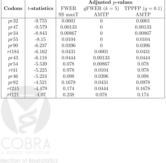
Procedure 1 is applied to obtain a bootstrap estimate Q0n of the test statistics null distributionQ0(withB = 7,500 bootstrap iterations). This es-timated null distribution is used to compute adjustedp-values for the FWER-controlling single-step maxT MTP (Equation (13), Procedure 2). These FWER-controlling p-values are then used to obtain adjusted p-values for augmentation procedures controlling gFWER (k = 5) and TPPFP (q= 0.1) (for gFWER control, Equation (20), Procedure 6, and for TPPFP control, Equation (22), Procedure 7).
4.3
Software implementation in SAS
The multiple testing procedures implemented in the SAS macros of Section 3 can be applied to the HIV-1 (or a similar) dataset as follows. The param-eter values specified below are those for the particular analysis of the HIV-1 dataset reported in Section 4.4 (see code in the Appendix).
1. Read in the data in the form of a SAS dataset [y:X], with first col-umn corresponding to an outcome Y (i.e., natural logarithm of viral replication capacity measure) and M subsequent columns to an M– dimensional covariate vector X = (X(m) :m= 1, . . . , M) (i.e., binary codon genotypes).
2. Define the following parameters:
– the number of rows (i.e., patients) for the dataset[y:X], n= 317
(macro variable&row);
– the number of columns,M + 1 = 283 (macro variable &col);
– the number of bootstrap iterations for estimating the test statistics null distribution, B = 7,500 (macro variable&boots);
– the allowed number of false positives for the gFWER-controlling AMTP, k = 5 (macro variable&k);
– the allowed proportion of false positives for the TPPFP-controlling AMTP, q= 0.1 (macro variable &q);