DEPARTEMENT TOEGEPASTE
ECONOMISCHE WETENSCHAPPEN
RESEARCH REPORT 9915
ON MAXIMIZING THE NET PRESENT VALUE OF A PROJECT UNDER RESOURCE
CONSTRAINTS by M.VANHOUCKE E. DEMEULEMEESTER W. HERROELEN 0/1999/2376/15
PROJECT UNDER RESOURCE CONSTRAINTS
Mario V ANHOUCKE • Erik DEMEULEMEESTER. Willy HERROELEN
March 1999
Operations Management Group Department of Applied Economics
Katholieke Universiteit Leuven Naamsestraat 69, B-3000 Leuven (Belgium)
Phones: 32-16-326965,32-16-326972,32-16-326970, Fax 32-16-32 6732 E-mail: <firstname>.<name>@econ.kuleuven.ac.be
Mario V ANHOUCKE • Erik DEMEULEMEESTER. Willy HERROELEN ABSTRACT
In this paper we study the resource-constrained project scheduling problem with discounted cash flows. Each activity of this resource-constrained project scheduling problem has resource requirements for each resource type and a known deterministic cash flow which can be either positive or negative. Cash flows are assumed to be known in both their amount and timing. Progress payments and cash outflows occur at the completion of activities. The objective is to schedule the activities subject to a fixed deadline in order to maximize the net present value (npv) subject to the precedence and resource constraints.
With these features the financial aspects of project management are no longer ignored. We introduce a depth-first branch-and-bound algorithm which makes use of extra precedence relations to solve a number of resource conflicts and a fast recursive search algorithm for the max-npv problem to compute the upper bounds. The recursive search
algorithm exploits the idea that positive cash flows should be scheduled as early as possible while negative cash flows should be scheduled as late as possible within the precedence constraints. The procedure has been coded in Visual C++, version 4.0 under Windows NT and has been validated on three randomly generated problem sets.
Keywords: Resource-constrained project scheduling; Discounted cash-flows; Branch-and-bound
1. Introduction
In recent years a number of publications have dealt with the project scheduling problem under the objective of maximizing the net present value (npv) of the project. The majority of the contributions assume a completely deterministic project setting, in which all relevant problem data, including the various cash flows, are assumed known from the outset. Research efforts have led to exact procedures for the unconstrained project scheduling problem, where activities are only subject to precedence constraints. In
addition, numerous efforts aim at providing optimal or suboptimal solutions to the project scheduling problem under various types of resource constraints, using a rich variety of often confusing assumptions with respect to network representation (activity-on-the-node versus activity-on-the-arc), cash flows patterns (positive andlor negative, event-oriented or activity-based), and resource constraints (capital constrained, different resource types, materials considerations, time/cost trade-offs). A number of efforts focus on the simultaneous determination of both the amount and timing of payments. Last, a modest start has been taken in tackling the stochastic aspects of the scheduling problem involved. For a recent review of the vast literature and a categorization of the solution procedures, we refer the reader to Ozdamar and Ulusoy (1995) and Herroelen et al. (1997).
In this paper we present a branch-and-bound algorithm to maximize the net present value (npv) in project networks with zero-lag finish-start precedence constraints and renewable resource constraints (problem m,
11
cpm, On,CjI
npv following the classification scheme of Herroelen et al. (1998) and further denoted as RCPSPDC, i.e. the Resource~onstrained Eroject ~cheduling Eroblem with .Qiscounted ~ash flows). The proposed
solution procedure makes use of a fast recursive search algorithm for the unconstrained max-npv project scheduling problem (problem cpm,On,Cj
I
npv, further denoted as the max-npv problem) to compute the upper bounds, which we will also discuss in the following of this paper.The branch-and-bound procedure makes use of the concept of minimal delaying alternatives that was introduced by Demeulemeester and Herroelen (1992, 1997) and additional precedence relations to resolve resource conflicts due to Icmeli and Erengii<; (1996). Algorithms for the max-npv problem have been presented by Russell (1970), Grinold (1972), Elmaghraby and Herroelen (1990), Herroelen and Gallens (1993), Kazaz and Sepil (1996), Etgar et al. (1996), Shtub and Etgar (1997) and Etgar and Shtub (1999). Exact algorithms for the RCPSPDC have been presented by Doersch and Patterson (1977), Smith-Daniels and Smith-Daniels (1987), Patterson et al. (1989, 1990), Baroum (1992), Yang et al. (1992), Icmeli and Erengii<; (1996) and Baroum and Patterson (1999). Heuristic approaches have been presented by Russell (1986), Smith-Daniels and Aquilano (1987), Padman and Smith-Daniels (1993), Icmeli and Erengti<; (1994), Ozdamar et al. (1994), Yang et al. (1995), Ulusoy and Ozdamar (1995), Baroum and Patterson (1996), Pinder and Marucheck (1996), Dayanand and Padman (1996), Smith-Daniels et al. (1996), Zhu and Padman (1996), Padman et al. (1997), Sepil and Orta<; (1997) and Zhu and Padman (1997). The organisation of the paper is as follows. In section 2 we discuss the max-npv problem. Section 3 reviews the recursive search algorithm for the max-npv problem. In
section 4 we discuss the RCPSPDC. Section 5 describes a branch-and-bound approach for this RCPSPDC. Section 6 is reserved for an illustration by means of a numerical example and in section 7 we report detailed numerical results on three problem sets. In section 8 we describe our overall conclusions.
2. The deterministic max-npv problem
The detenninistic max-npv problem involves the scheduling of project activities in order to maximize the net present value (npv) of the project in the absence of resource constraints. The project is represented by an activity-on-the-node (AoN) network G=(N,A)
where the set of nodes, N, represents activities and the set of arcs, A, represents finish-start precedence constraints with a time lag of zero. The activities are numbered from the dummy start activity 1 to the dummy end activity n. The duration of an activity is denoted
by d; (1 :,; i :,; n) and the performance of each activity involves a series of cash flow payments and receipts throughout the activity duration. Assume that
cli,
(1 < i < n) denotes the known deterministic cash flow of activity i in period t of its execution. A terminal value of each activity upon completion can be calculated by compounding the associatedd;
cash flow to the end of the activity as follows: ci =
I,
Cfilea(d;-I) , where IX represents the 1=1discount rate and Ci the tenninal value of cash flows of activity i at its completion. If the nonnegative integer variable
li
(1 :,; i :,; n) denotes the completion time of activity i, its discounted value at the beginning of the project is cie-ajj . A formulation of the max-npv problem can be given as follows:n-l Maximize
I,
ci e -a j; i=2 Subject tof :,;
f
j -dj fn :';0n fl =0 't:/(i, j) E A [1][2]
[3][4]
The objective in Eq. 1 maximizes the net present value of the project. The constraint set given in Eq. 2 maintains the finish-start precedence relations among the activities. Eq. 3 limits the project duration to a negotiated project deadline
On
and Eq. 4 forces the dummy start activity to end at time zero.The exact solution procedures for solving the max-npv problem which have been
offered in the literature take an event-oriented view with net cash flows associated with the events in AoA networks. Russell (1970) was the first to offer a nonlinear programming formulation and an exact solution procedure based on an iterative series of linear approximations and the solution of a transhipment problem over a network model. Apart from an example illustrating the application of the algorithm, he does not report on computational experience. Grinold (1972) also takes an event-oriented view and shows that the problem can be transformed into an equivalent linear program. Again, apart from an example illustrating the computations, no further computational results are given. Elmaghraby and Herroelen (1990) have developed an exact solution procedure for AoA networks based on the intuitive argument that positive cash flows should be scheduled as early as possible and negative cash flows should be scheduled as late as possible within the precedence constraints. The algorithm operates by building tree structures in an iterative fashion and by determining proper displacement intervals for the trees. Herroelen and Gallens (1993) have streamlined the algorithm and report on favorable computational results on 250 randomly generated projects with a computer code written in the C language and running under the DOS operating system. Kazaz and Sepil (1996) have presented a
MIP formulation for problems where cash flows do not occur at some event realization time, but as progress payments at the end of some time periods. Etgar et al. (1996), Shtub and Etgar (1997) and Etgar and Shtub (1999) have solved the max-npv problem for the case where net cash flow magnitudes are dependent of the time of realization.
In the next section we discuss the exact recursive search procedure for the max-npv problem as formulated above in Eqs. [1] -[4].
3. An exact recursive search procedure for the max-npv problem
In this section we will discuss the recursive search procedure for the max-npv. This algorithm will be used by the branch-and-bound procedure of section 5 to compute the upper bounds on the net present value of a resource-constrained project scheduling problem with discounted cash flows where the activities are also subject to renewable resource constraints.
The proposed recursive algorithm consists of three steps: the construction of an early tree, the construction of a current tree and a recursive search on the current tree.
3.1 Step 1: Constructing the early tree
The algorithm starts in step 1 by computing the earliest completion time for the activities based on traditional forward pass critical path calculations and determines the corresponding early tree, ET. Usingjj to denote the earliest finish time of activity j and Pj to denote the set of its immediate predecessors, the pseudocode of the forward pass procedure can be written as follows:
procedure forward_pass; ET=0; 11 :=0; Do for j := 2 to n-l jj:= 0; Do Vi E Pj
IfJi
+ dj > jj thenjj :=Ji
+ dj and i* := i;ET=ETu(i* j);
3.2 Step 2: Constructing the current tree
The early tree spans all activities scheduled at their earliest completion times and corresponds to a feasible solution with a project duration equal to the critical path length.
In step 2 the algorithm builds the current tree, CT, by delaying, in reverse order, all activities i with a negative cash flow and no successor in the early tree as much as possible within the early tree, i.e. by linking them to their earliest starting successor. We also add an extra arc to the current tree leading from the dummy end activity n, which is scheduled at the deadline of the project, to the dummy start activity 1. As explained later in this section, this extra arc is needed in order to allow the recursive search to be performed in the third step to start from the dummy start node. When Sj denotes the set of the immediate
successors of activity j, the pseudocode of the backward pass procedure to compute the current tree can be written as follows:
procedure backward_pass; in:= On; CT=ETu(n, 1); Do for j := n-1 to 2 If Cj < 0 and ~3kl (j,k) E CT thenfj:= 00; Do ViESj
Iff; -di <fj thenfj := f; -di and i* := i;
CT=CTu(j,i*);
CT=CT\(lj) with l E Pj
I
(l, j) E CT; 3.3 Step 3: Searching the current treeIn step 3 the current tree is the subject of a recursive search (starting from the dummy start activity 1) in order to identify sets of activities (SA) that might be shifted forwards (away from time zero) in order to increase the net present value of the project. Due to the structure of the recursive search it can never happen that a backward shift (towards time zero) of a set of activities can lead to an increase in the npv of the project.
When a set of activities SA is found for which a forward shift leads to an increase of the npv, the algorithm computes its displacement interval and updates the current tree
CT as follows. The arc (iJJ which connects a node i
e:
SA to a node j E SA in the currenttree CT is removed from it. The displacement interval of the set of activities SA under consideration is computed as follows. Find a new arc (k*,l*) for which
vk *[* = min {f[ - d[ -
i
k } and add it to the current tree. The completion times of the(k.l)EA kESA
[eSA
activities of SA are then decreased by the minimal displacement vk*[* and the algorithm
repeats the recursive search. IT no further shift can be accomplished, the algorithm stops and the completion times of the activities of the project with its corresponding npv is reported.
Using CA to denote the set of already considered activities and DC to denote the discounted cash flow of a set of activities SA, the third step, including the recursive algorithm, can be written as follows:
procedure Step_3; CA = 0;
Do RECURSJON(1) ~SA', DC' (parameters returned by the recursive function);
Report the optimal completion times of the activities and the net present value
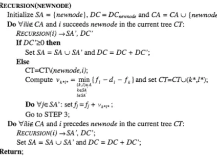
RECURSION(NEWNODE)
Initialize SA = {newnode}, DC = DCnewnode and CA = CA u {newnode}; Do Vilie; CA and i succeeds newnode in the current tree CT:
RECURSION(i) ~SA', DC'
If DC'?O then
Set SA = SA uSA' and DC = DC + DC'; Else
CT=CT\(newnode, i);
Compute Vk*I' = min {fl - dl - !k} and set CT=CTu(k*,I*);
(k'/)~A
keSA I.SA'
DoVjESA': setjj=jj+ vk'I';
Go to STEP 3;
Do Vilie; CA and i precedes newnode in the current tree CT: RECURSION(i) ~SA', DC';
Set SA = SA u SA' and DC = DC + DC'; Return;
As mentioned earlier, the extra arc leading from the dummy end activity n to the
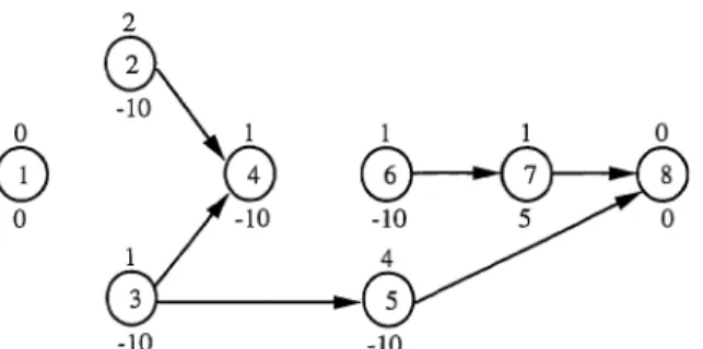
dummy start activity 1 in the current tree guarantees that there exists always a path in the current tree between each activity and activity 1, which allows each recursive search of the third step to start with activity 1. Without this extra arc, the algorithm may miss the optimum. To illustrate this point, consider the AoN project network given in Fig. 1. There are 6 activities and two dummy activities, each with an activity duration denoted above the node and a cash flow denoted below the node. The project deadline On is 7.
2
d;
o
C;Fig. 1. An example project network
Without the extra arc between activity n and activity 1, the solution of the recursive
recursive search algorithm is!] = 0,12 = 3,13 = 3,14 = 4,15 = 7,16 =
6,17
= 7,18 = 7. This solution, with a current tree given in Fig. 2, is clearly not optimal. Activities 2 and 4 should be shifted forward to increase the npv of the problem, However, due to the absence of a link between activity 1 and these activities, the recursive search will not make this happen. When we add the arc between activity 8 and 1, the recursive search will make the shift, leading to the optimal solution with!] = 0,12 = 4,f3 = 3,14 = 5,f5 = 7,f6 =6,17
= 7,f8 = 7 with the corresponding current tree as given in Fig. 3.2 0
~
1 1 0CD
G
6~_10
0 1 4 3 5 -10 -10Fig. 2. Final solution obtained when the current tree does not contain the extra arc (n,1)
2
7
cb~---.~~
-10 -10Fig. 3. Optimal solution when the extra arc (n,l) is added to the current tree
4. The deterministic RCPSPDC
The RCPSPDC differs from the max-npv problem in the use of resources for the different activities. There are K renewable resources with constant availability ak (1 ::; k ::; K). Let rik (1 ::; i ::; n, 1 ::; k ::; K) denote the resource requirements of activity i with respect to resource type k. The deterministic resource-constrained project scheduling problem with discounted cash flows involves the scheduling of the project activities in order to maximize the net present value subject to the precedence and resource constraints.
The RCPSPDC can be conceptually formulated as follows: n-I
Maximize L,cie-afi
i=2 Subject to J; ::;
i
j -dj L,rik ::;a k iES(t)il
=0in::;
8n
ii
EN V(i,j) E A k = 1,2, ... ,K t = 1,2, ... ,8n i = 1,2, ... ,n [5][6]
[7]
[8] [9] [10]where Set) denotes the set of activities in progress in period ]t-1,t]. The objective in Eq. 5 maximizes the net present value of the project. The constraint set given in Eq. 6 maintains the finish-start precedence relations among the activities. Eqs. 7 represent the resource constraints while Eq. 8 forces the dummy start activity to end at time zero. Eq. 9 limits the project duration to a negotiated project deadline On and Eqs. lO ensure that the activity finishing times assume nonnegative integer values.
Among the exact algorithms for solving the RCPSPDC (Herroelen et al., 1997) the branch-and-bound procedure of Icmeli and ErengU~ (1996) is reported to be the most efficient. The algorithm extends the resource-constrained project scheduling algorithm of Demeulemeester and Herroelen (1992) by adapting the branching strategy to cope with the
max-npv criterion. Bounds are computed by solving unconstrained max-npv problems
using the procedure of Grinold (1972). The authors have tested their algorithm on 50 Patterson problems (Patterson, 1984) and 40 problems generated by ProGen (Kolisch et al., 1995) and have shown that it outperforms the exact procedure of Yang et al. (1992). In
the next section we describe a branch-and-bound algorithm which outperforms the Icmeli
and Erengii~ procedure.
5. The branch-and-bound algorithm
5.1 Description of the search tree and branching strategy
At the initial node of the branch-and-bound tree, we relax the problem by dropping the resource constraints of Eqs. [7] and exploit the fact that the optimal solution to the resulting unconstrained max-npv problem yields an upper bound ub. If the solution obtained by the recursive search procedure described in section 3 is resource feasible, we have found the optimal solution for the RCPSPDC and the procedure terminates. If,
however, the solution shows a resource conflict, we branch into the next level of the branch-and-bound tree to generate a set of delaying alternatives. A resource conflict occurs
when there is at least one period ]t-1,t] for which 3k ::::; K:
L
rik > ak • A delayingiES(t)
alternative is a set of activities which, if delayed, resolve the resource conflict. According to Demeulemeester and Herroelen (1992, 1997), only minimal delaying alternatives must be considered to resolve a resource conflict. A delaying set DS, containing one or more delaying alternatives, can give rise to several minimal delaying modes (De Reyck and Herroelen, 1998). For each delaying mode of the minimal delaying set DS, we append additional precedence relations to resolve the resource conflict (Icmeli and ErengU~, 1996) and compute a new upper bound using the recursive search procedure of section 3. If, for example, activities 1, 2 and 3 cause a resource conflict and the delaying set contains two delaying alternatives, i.e. DS = {{ 1,2}, {3} }, then the three different delaying modes are (1-< 3), (2-< 3) and (3 -< 1,2) corresponding to four additional precedence relations. Each delaying mode corresponds to a node in the branch-and-bound tree which will be further explored during the branching process. We select among these nodes the delaying mode with the largest ub. If, on the one hand, the upper bound of a node corresponds to a solution which is resource feasible, we update the lower bound lb of the project (initially set to -00) and explore the next delaying mode at this level. If, on the other hand, the upper bound of a node is lower than or equal to the current lower bound, we fathom this node
and backtrack to the previous level of the search tree. If the upper bound is greater than the current lower bound, we generate a new set of delaying alternatives at the next level of the tree. If there are no delaying modes left unexplored, we backtrack and proceed in the same way at the previous level. The algorithm stops when we backtrack to the initial level of the branch-and-bound tree.
5.1 Node fathoming rules
Essentially, each node in the branch-and-bound tree represents the initial project network extended with a set of zero-lag finish-start precedence constraints to resolve resource conflicts. Therefore, it is possible that a certain node represents a project network which has been examined earlier at another node in the branch-and-bound tree. One way of checking whether two nodes represent the same project network is to check the added precedence constraints. If a node is encountered for which the set of added precedence constraints is identical to the set of precedence constraints associated with a previously
examined node, the node can be fathomed. Moreover, the subset dominance rule
developed by De Reyck and Herroelen (1998) for the resource-constrained project scheduling problem with generalized precedence relations also holds for the RCPSPDC and can be applied when a node is compared to a previously examined node in another path in the branch-and-bound tree:
Subset dominance rule:
If
the set of added precedence constraints which leads to the project network in node x contains as a subset another set of precedence constraints leading to the project network in a previously examined node y in another branch of the search tree, node x can be fathomed.Since the detection of a dominated subset goes much faster than the calculation of an upper bound, we first check if the node can be dominated by a previously examined node. Only if the node cannot be fathomed due to the subset dominance rule, we calculate an upper bound. The information that is needed to test this dominance rule can be efficiently saved on a stack as follows. When the procedure backtracks to a node at level p, all the required information for dominance testing which has been saved at level p + 1 will be removed from the stack and the added precedence relations of that node will be saved on the stack. In doing so, only the necessary information is saved on the stack while the superfluous information is removed again and again. Clearly, as mentioned earlier, a node can also be fathomed when its upper bound is lower than or equal to the current lower bound or when its solution is resource feasible. Of course, in the last case, the lower bound has to be updated first.
5.3 The algorithm
When ACz denotes the set of added precedence constraints in node z (with respect to the original set of precedence constraints A) and x is used to denote the current node in the branch-and-bound tree, the detailed steps of the branch-and-bound algorithm can be written as follows:
STEP 1.INmALISATION
• Let lb
= -
co be the lower bound on the net present value of the project. • Initialize the level of the branch-and-bound tree: p = O.• Relax the problem and compute an upper bound ub on the npv using the recursive solution procedure of section 3.
• If this solution is resource feasible, i.e. for each period ]t-l ,t] and
'v'k:5. K: ~>ik :5. ak , STOP. iES(t)
• Go to STEP 2.
STEP 2. MINIMAL DELAYING ALTERNATIVES
• Increase the level of the branch-and-bound tree: p = p + 1.
• Determine the minimal delaying setDS (which contains the minimal delaying alternatives DA) and its corresponding set of delaying modes MS (which contains the delaying modes DM):
DS= {DAIDAcS(t) and 'v'k:5.K: I,rik :5.ak and ~3jEDAI I,rik +rjk :5.ak }
iES(t)'DA iES(r)'DA
MS = {DMlDM= (k-<. DA), kES(t)\DA andDAEDS}.
• Delete all minimal delaying modes satisfying the subset dominance rule, i.e. MS = MS\{DMlACyc(ACuDM)} with y a previously examined node in the branch-and-bound tree.
• Compute for each non-dominated delaying mode an upper bound ub on the npv using the recursive solution procedure of section 3.
• Delete all minimal delaying modes for which ub :5.lb, i.e. MS
=
MS\{DMIub :5.lb}. • Go to STEP 3.STEP 3. RESOURCE ANALYSIS
• Do for each non-dominated delaying mode:
- Determine the first period in the optimal schedule in which a resource conflict
occurs, i.e. the first period ]t-l ,t] for which 3k :5. K:
I,
rik > ak . iES(r)- If there is no resource conflict and ub > lb, update lb
=
ub. • Go to STEP 4.STEP 4. BRANCHING
• If there are no delaying modes left at this levelp with ub > lb, go to STEP 5. • Select the delaying modeDMEMS with the largerst ub and add the additional
precedence relations, i.e. ACx = ACuDM. • Go to STEP 2.
STEP 5. BACKTRACKING
• Delete the additional precedence relations inserted at levelp, i.e. ACx = ACx\DM. • Decrease the level of the branch-and-bound tree: p
=
p - 1.6. An example
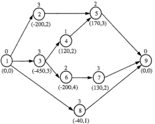
In this section we will compute the optimal solution by means of an example from the Patterson set (Patterson, 1984). Consider the AoN project network given in Fig. 4. There are 7 activities (and two dummy activities) and one resource type with a constant availability of 5. The number above the node denotes the activity duration, while the numbers below the node denote the cash flow and the resource requirements, respectively. The discount rate ex is 0.01 and the project deadline On is 12.
3 2 )---I~ 2
0
-(-20Q,4) dio
(Ci' r;)Fig. 4. A project network from the Patterson set
The branch-and-bound tree for the example is given in Fig. 5. The number in bold denotes the number of the node in the search tree, while the two other lines denote the additional precedence relations and the upper bound obtained by the recursive search algorithm, respectively. At the initial level p = 0, the npv-value of the optimal solution obtained by the recursive procedure is ub = -441.96 with finishing times!2 = 1O,f3 = 7,14 =
8,f5 = 12,f6 = 9,17 = 12 andfs = 12. Since activities 2, 4 and 6 cause a resource conflict at time instant 8, we determine the minimal delaying set at the next level of the branch-and-bound tree. DS = {{ 2,4 }, {6}} and therefore, we create 3 delaying modes (with three additional precedence relations) corresponding to the three new nodes 2, 3 and 4 at level p = 1. For each node we compute an upper bound. We select the delaying mode with the largest upper bound, i.e. node 2 with ub = -445.06 and finishing times!2 = 10,/3 = 6,14 =
7,J5 = 12,16
=
9,17 = 12 andfs = 12. Since activities 2 and 6 cause a resource conflict at time instant 8, the solution of this node is not resource feasible. We generate DS ={ {2}, { 6}} and 2 delaying modes corresponding to nodes 5 and 6 at the next level p = 2. Remark that the solution of node 6 is resource feasible. We update the current lower bound lb = -452.73. We explore the delaying mode with the largest upper bound, i.e. node 5 with ub
=
-445.98 and finishing times!2 = 7,13 = 6,/4 = 7,J5 = 9,J6 = 9,17 = 12 andfs=
12. Since the resource requirements at time instant 8 exceed the resource availibilities, we generate DS= {
{5}, { 6} } and 2 delaying modes corresponding to nodes 7 and 8 at the next level p = 3 of the search tree. Upon computing an upper bound for both nodes, we can fathom node 7 because the upper bound is lower than the lower bound. We proceed withnode 8, for which the max-npv solution is not resource feasible, since activities 5, 7 and 8 have a resource requirement of 6 at time instant 10. Since DS = {{5},{7},{8}}, we generate six new nodes at level p = 4 and compute the corresponding upper bounds. All nodes except node 11 can be fathomed. Node 11 is resource feasible and its upper bound ub
=
-450.14 is greater than the lower bound lb=
-452.73, which makes it the best solution currently found. We update the lower bound lb = -450.14. Since there are no nodes left unexamined at level p = 4, we backtrack until we reach a level containing unexamined nodes. The procedure backtracks to level p = 1 and selects the first unexamined node which has the largest upper bound, i.e. node 3 at level 1. The algorithm continues this way until it returns at the initial node at level O. Notice that no upper bound is computed in node 17, because it is fathomed by node 2 due to the subset dominance rule, denoted by D2in Fig. 5. The optimal solution of the example has a net present value of -450.14 as given in node 11 of Fig. 5.
1
.1
91
i...JlL.l
1 1 ''L1LJ114
il.---!L.il2Li
ULJ
LRJ
I
23i
r
24!
'7-< 8
II
5-< 8I
8-< 7 ;d
8-< 5 1\7-< 5II
7-< 8II
5-< 8Ii
8-< 7II
5-< 7I
rs-:;s--i
I
7-< 5I
. -461.65d
-457.411 -450.14 ! -459.7411-450.14 11-462.0011-462.281! -462.28 iI-450.741 i -465.781i
-450.38 i!
-461.081ub ub lb = -450.14 ub ub ub ub ub ub ub ub ub
Fig. 5. The branch-and-bound tree
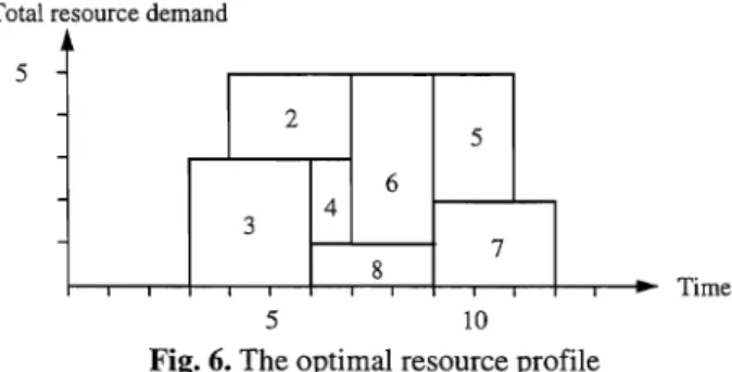
The resource profile of the optimal solution is given is Fig. 6. Project execution starts at time instant 3. The project terminates at time instant 9. Observe that this does not correspond to the optimal solution under the makespan objective, which would yield a makespan of 8.
Total resource demand 5
I
2 5 6 4 3 7 8 Time 5 10Fig. 6. The optimal resource profile
7. Computational experience
Both the exact recursive search algorithm for the max-npv problem and the branch-and-bound algorithm for the RCPSPDC have been coded in Visual C++ Version 4.0 under Windows NT 4.0 on a Dell personal computer (Pentium 200 MHz processor).
In order to validate both procedures, we used three different problem sets. For the validation of the max-npv problem, we generated 5,250 test instances with ProGenIMax (Schwindt, 1995). In order to validate our branch-and-bound algorithm for the RCPSPDC, we used two different problem sets. The first contains 110 problems from the well-known Patterson problem set (Patterson, 1984) and is used to compare our results with the ones found by Icmeli and Erengtic;: (1996). The second problem set consists of 47,520 problem instances generated by ProGenJMax (Schwindt, 1995).
The parameter settings of the instances of the different problem sets in activity-on-the-node format are described in the subsequent sections. All problem sets were extended with cash flows, a discount rate
a
and a project deadline bn .The project deadlines for the instances in problem set I were set 100 units above the critical path length, while the project deadlines for the instances in problem sets II and
ill were generated as follows. After solving the different test instances with the procedure of Demeulemeester and Herroelen (1997) to obtain the minimal makespan, we generate the project deadline bn by increasing the minimal makespan with a number as described in sections 7.2 and 7.3.
7.1 Problem set I: Computational experience for the max-npv problem
Table I represents the parameter settings used to generate the test instances for the max-npv problem. The parameters used in the full factorial experiment are indicated in bold. These instances in activity-on-the-node format use four settings for the number of activities and three settings for the order strength OS. The order strength, OS (Mastor,
1970), is defined as the number of precedence relations (including the transitive ones) divided by the theoretical maximum of number of precedence relations (n(n-1 )/2, where n denotes the number of activities). We provided the problems with cash flows, a discount factor a and a deadline bn . The cash flows were randomly generated from the interval [-500;500]. Using 10 instances for each problem class, we obtain a problem set with 5,280 test instances
Table I. Parameter settings used to generate the test instances for the max-npv problem
Number of activities 30, 60, 90 or 120 Activity durations
Number of initial and terminal activities Maximal number of successors and predecessors Order strength OS
randomly selected from the interval [1,10] randomly selected from the interval [2,4] 4
0.25, 0.50 or 0.75 (Mastor, 1970)
Discount rate a (in %) Percentage negative cash flows Deadline ofthe project 8n
0.20, 0.40, 0.80 or 1.60
0%, 10%, 20%, 30%, 40%, 50%, 60%, 70%, 80%, 90% or 100%
critical path length + 100
The average CPU-time and the standard deviation for the max-npv problem are reported in milliseconds in Tables II through IV (actually, we have solved 1,000 replications for each problem and reported the time in seconds). Table II reveals that the recursive algorithm is very efficient. Even instances with 120 activities can be solved with an average CPU-time of 1.588 milliseconds. The required computational effort by the recursive search procedure is sufficient small to allow the efficient computation of an upper bound for the undominated nodes in the branch-and-bound tree for the RCPSPDC which may run in the thousands (even millions).
Table II. Impact of the number of activities # activities 30 60 90 120 # problems 1,320 1,320 1,320 1,320 Average CPU-time 0.130 0.450 0.850 1.577 Standard Deviation 0.101 0.356 0.788 1.453
Table ill shows a positive correlation between the OS of a project and the required CPU-time, i.e. the more dense the network, the more difficult the problem.
Table III. Impact of the order strength
OS # problems Average CPU-time Standard Deviation
0.25 1,760 0.564 0.645
0.50 1,760 0.730 0.909
0.75 1,760 0.961 1.306
In correspondence with the results found by Icmeli and Erengii<;: (1996) for the RCPSPDC, Table IV reveals that the discount rate did not have a significant impact on the performance of the algorithm.
Table IV. Impact of the discount rate Discount rate # problems
0.2 1,320 0.4 1,320 0.8 1,320 1.6 1,320 Average CPU-time 0.730 0.737 0.755 0.786 Standard Deviation 0.986 0.994 1.009 1.030
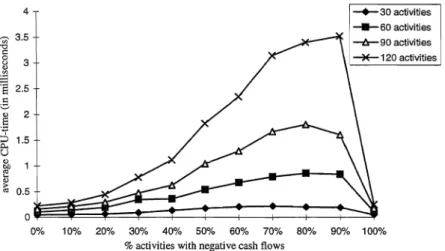
Fig. 7 shows the impact of the percentage of negative cash flows on the required CPU-time for a different number of activities. If, on the one hand, all the activities have a positive cash flow, the optimal solution of the max-npv problem consists of scheduling the activities as early as possible, without performing any shift towards the deadline. If, on the other hand, all the cash flows are negative, the opposite is true: all the activities are scheduled nearby the deadline. When the activities can have either positive or negative cash flows, the problem becomes harder. The higher the percentage negative cash flows in the project, the more shifts are needed to solve the max-npv problem to optimality.
4 -;)' 3.5 '0 c o ~ 3
's
2.5 --+-30 activities --11-60 activities 0% 10% 20% 30% 40% 50% 60% 70% 80% 90% 100%% activities with negative cash flows
Fig 7. Effect of the % of negative cash flows for a different number of activities
7.2 Problem set II : Computational experience for the RCPSPDC on the Patterson problem set
Icmeli and Erengiic;: (1996) have assembled a problem set containing 90 instances to run on an IBM3090 computer with vector processor. Fifty of the test problems came from the set that was assembled by Patterson (1984) while the other forthy problems were generated by ProGen (Kolisch et al., 1995). Each problem instance was extended with a deadline and a randomly generated cash flow from a uniform distribution between [-5000; 10,000] which means that, on the average, 33% of the activities have a negative cash flow. When the deadlines of the problem instances were set to three time units above the minimal makespan, 36 of the 50 instances from the Patterson set could be solved to optimality within a time limit of 600 seconds and a maximum of 4,000 subproblems. This number decreased when the project deadline was set, on the average, fourteen units above the minimal makespan: 17 of the 50 Patterson instances could be solved to optimality within the limits of 600 seconds and 4,000 subproblems. Using our branch-and-bound procedure, a total of 46 of the 50 Patterson instances could be solved to optimality within a time limit of 100 seconds when the project deadline is 3 time units above the makespan. When the deadline is set to 14 time units above the minimum makespan, the number of optimally solved problems amounts to 46. The average CPU-time for the problems that were solved to optimality is 13.35 seconds (with a standard deviation of 31.08) and 10.77
seconds (and a standard deviation of 29.09), respectively. Clearly, our procedure outperforms the one by Icmeli and Erengti~ (1996).
Table V represents the average CPU-time and the percentage of optimally solved problems within different time limits for the entire 110 Patterson problem set with a cash flow distribution and project deadlines as described in Table VI. 56 % of the problems could be solved within 1 second, while 87 % of the problems were solved to optimality within a time limit of 100 seconds.
Table V. Results for different time limits of CPU-time in seconds for the entire Patterson problem set
time limit # problems Average CPU-time % solved to optimality 6,050 10 6,050 100 6,050 0.533 3.282 17.397 56 % 75% 87 %
7.3 Problem set III : Computational experience for the RCPSPDC
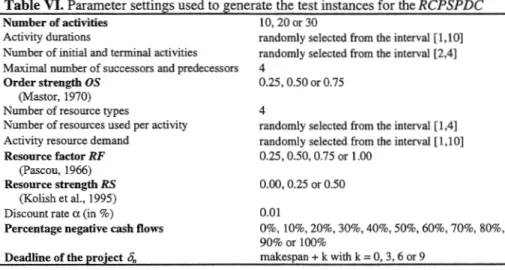
Table VI represents the parameter settings used to generate the test instances for the RCPSPDC. The parameters used in the full factorial experiment are indicated in bold.
We obtained 4,752 problem classes, each consisting of 10 instances.
Table VI. Parameter settings used to generate the test instances for the RCPSPDC
Number of activities 10, 20 or 30
Activity durations
Number of initial and terminal activities Maximal number of successors and predecessors Order strength OS
(Mastor, 1970) Number of resource types
Number of resources used per activity Activity resource demand
Resource factor RF
(Pascou, 1966) Resource strength RS
(Kolish et aI., 1995) Discount rate ex (in %) Percentage negative cash flows Deadline of the project On
randomly selected from the interval [1,10] randomly selected from the interval [2,4] 4
0.25,0.50 or 0.75
4
randomly selected from the interval [1,4] randomly selected from the interval [1,10] 0.25,0.50,0.75 or 1.00 0.00, 0.25 or 0.50 0.01 0%, 10%, 20%, 30%, 40%, 50%, 60%, 70%, 80%, 90% or 100% makespan + k with k = 0, 3, 6 or 9
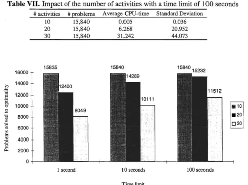
Table VII represents the average CPU-time and its standard deviation in seconds for a different number of activities with a time limit of 100 seconds. Fig. 8 displays the number of problems solved to optimality for a different number of activities and allowed time. Clearly, the number of activities has a significant effect on the average CPU-time and on the number of problems solved to optimality. Almost all problems with 10 activities can be solved to optimality within 1 second of CPU-time. For problems containing 20 activities, 78.3% of the number of problems can be solved to optimality when the allowed CPU-time is 1 second, whereas 96.2% of the number of problems can be optimally solved when the time limit is 100 seconds (with an average CPU-time of 6.268
seconds). For problems with 30 activities, 50.8% of the number of problems can be solved within 1 second of CPU-time whereas 72.7% of the number of problems can be solved to optimality when the allowed CPU-time is 100 seconds (with an average CPU-time of 31.242 seconds).
Table VII. Impact of the number of activities with a time limit of 100 seconds
# activities # problems Average CPU-time Standard Deviation
10 15,840 0.005 0.036 20 15,840 6.268 20.952 30 15,840 31.242 44.073 15835 15840 1584015232 16000 0 14000 ~ 12000 E "g. 10000 1110 0
.s
.20 -0 8000"
..e; 030 Sl 6000~
4000 :0£
2000 01 second 10 seconds 100 seconds
Time limit
Fig. 8. Effect ofthe number of activities
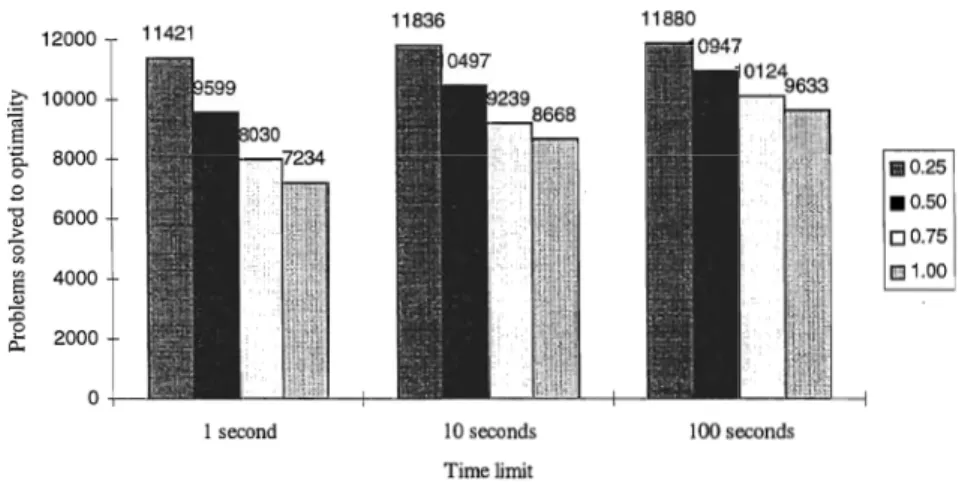
The effect of OS on the number of problems solved to optimality is displayed in Fig. 9. Despite the fact that higher OS values yield harder max-npv instances (see Table
III), the order strength has a negative correlation with the hardness of the RCPSPDC, that
16000 .£ 14000 -a 12000 .§ "-0 10000 8 "0 8000 "
,.
~E
6000"
4000 :0"
~ 2000 a 155841 second 10 seconds 100 seconds
Time limit
Fig. 9. Effect of the order strength (OS)
ill 0.25 .0.50 00.75
Fig. 10 and Fig. 11 display the effect of the resource factor (RE) and the resource strength (RS), respectively, on the number of problems solved to optimality within an allocated CPU-time. The results confirm earlier results already found by Kolisch et al. (1995) and De Reyck and Herroelen (1998). The higher the resource factor, the more difficult the instances, while the opposite holds for the resource strength.
12000 .-2 10000 -a
a
.';5. 8000 o 6000§
4000 :0£
2000 a 1 second 10 seconds Time limit 100 secondsFig. 10. Effect of the resource factor (RE)
ill 0.25 .0.50 00.75 IE 1.00
16000 .g 14000
'"
S 12000 oR 0 10000 .9 -0 8000 QJ > S1 E 6000 QJ 4000 :0 8 ~ 2000 01 second 10 seconds 100 seconds
Time limit
Fig. 11. Effect of the resource strength (RS)
BlO.OO .0.25 00.50
Fig. 12 illustrates the impact of the cash flow distribution on the average CPU-time with different project deadlines. It appears that, when the project deadline is high enough, instances with few or many activities with a negative cash flow are the most difficult to solve. This is due to the fact that in these cases resource conflicts will occur very often. When there are both activities with positive and negative cash flows, the chance that a resource conflict occurs diminishes since the problem now contains activities scheduled at the beginning of the project as well as activities scheduled nearby the deadline. Although we have observed an opposite effect for the max-npv problem, the impact of the deadline on the resources seems to be much stronger.
20 '" 18 -0
'"
0 16 u 1;l 14 c"'"
12"
S 10~
8 ~ U 6"
on 4e
"
2,.
'"
0 0 - - - - - - ------
- ---;.:~: ~ ... _ ...-
... "" ... ,.-,.
...,,"
- ... -10 20 30 40 50 60 70 80% activities with negative cash flows
- - - - deadline k=O ••••••• deadline k=3 - - deadline k=6 - •• _. deadline k=9
90 100
8. Conclusions
In this paper we presented a branch-and-bound procedure for the resource-constrained project scheduling problem with discounted cash flows (RCPSPDC;
m,ll
cpm, On, CjI
npv) based on a fast recursive search algorithm for the max-npv problem(cpm,
on,
CjI
npv). Each activity ofthis resource-constrained project scheduling problem has a known deterministic cash flow and constant resource requirements for each renewable resource type. The objective is to schedule the activities in order to maximize the net present value of the project without violating the availabilities of the resources and subject to a project deadline. To the best of our knowledge, the procedure by Icmeli and Erengi.i<; (1996) is the best exact procedure currently available.The depth-first branch-and-bound algorithm uses a new fast recursive search algorithm for the max-npv problem to compute the upper bounds while resource conflicts are resolved through the introduction of additional precedence constraints as described by Icmeli and Erengi.i<; (1996). The branching strategy was extended with the subset dominance rule to prune the search tree considerably.
Both the recursive procedure for the max-npv problem and the branch-and-bound procedure have been coded in Visual C++, version 4.0 under Windows NT and have been tested on randomly generated problem sets. The results of extensive computational tests obtained on a Dell personal computer (Pentium 200 MHz) are encouraging. Unconstrained max-npv problems can be solved within a very small amount of CPU-time allowing for an efficient upper bound calculation. The promising results indicate that the branch-and-bound procedure is able to solve optimally instances up to 30 activities and 4 resource types in a reasonable time limit.
References
Baroum, S.M., "An exact solution procedure for maximizing the net present value of resource-constrained projects', unpublished Ph.D. Dissertation, Indiana University, 1992.
Baroum, S.M. and Patterson, I.H., 1999, "An exact solution procedure for maximizing the net present value of cash flows in a network", , in: Weglarz I. (Ed.), Handbook on Recent Advances in Project Scheduling, Kluwer Academic Publishers, Chapter 5, 107-134.
Baroum, S.M. and Patterson, I.H., 1996, "The development of cash flow weight procedures for maximizing the net present value of a project", Journal of Operations Management, 14,209 - 227.
Dayanand, N. and Padman, R., 1996, "A simulated annealing approach for scheduling payments in projects", Working Paper 94-90, Carnegie-Mellon University.
De Reyck, B. and Herroelen, W., 1998, "A branch-and-bound procedure for the resource-constrained project scheduling problem with generalized precedence relations", European Journal of Operational Research, 111, 125-174.
Demeulemeester, E. and Herroelen, W., 1992, "A branch-and-bound procedure for the multiple resource-constrained project scheduling problem", Management Science, 38, 1803-1818.
Demeulemeester, E. and Herroelen, W., 1997, "New benchmark results for the resource-constrained project scheduling problem", Management Science, 43,1485-1492.
Doersch, RH. and Patterson, J.H., 1977, "Scheduling a project to maximize its present value: A zero-one programming approach", Management Science, 23, 882-889.
Elmaghraby, S.E. and Herroelen, W., 1990, "The scheduling of activities to maximize the net present value of projects", European Journal of Operational Research, 49, 35-49.
Etgar, R., Shtub, A. and LeBlanc, LJ., 1996, "Scheduling projects to maximize net present value - the case of time-dependent, contingent cash flows", European Journal of Operational Research, 96, 90-96.
Etgar, Rand Shtub, A., 1999, "Scheduling project activities to maximize the net present value - the case of linear time dependent, contingent cash flows", International Journal of Production Research, 37, 329-339.
Grinold, RC., 1972, "The payment scheduling problem", Naval Research Logistics Quarterly, 19, 123-136.
Herroelen, W. and Gallens, E., 1993, "Computational experience with an optimal procedure for the scheduling of activities to maximize the net present value of projects",
European Journal of Operational Research, 65, 274-277.
Herroelen, W., Demeulemeester, E. and Van Dommelen, P., 1997, "Project network models with discounted cash flows: A guided tour through recent developments",
European Journal of Operational Research, 100, 97-12l.
Herroelen, W., Demeulemeester, E. and De Reyck, B., 1999, "A classification scheme for project scheduling problems", in: Weglarz J. (Ed.), Handbook on Recent Advances in Project Scheduling, Kluwer Academic Publishers, Chapter 1, 1-26.
Icmeli, O. and Erengiic;, S.S., 1994, "A tabu search procedure for resource-constrained project scheduling with discounted cash flows", Computers and Operations Research,
21,841-853.
Icmeli, O. and Erengiic;, S.S., 1996, "A branch-and-bound procedure for the resource-constrained project scheduling problem with discounted cash flows", Management Science, 42, 1395-1408.
Kazaz, B. and Sepi1,
c.,
B., 1996, "Project scheduling with discounted cash flows and progress payments", Journal of the Operational Research Society, 47,1262-1272.Kolisch, R, Sprecher, A. and Drexl, A., 1995, "Characterization and generation of a general class of resource-constrained project scheduling problems", Management Science, 41,1693-1703.
Mastor, A.A., 1970, "An experimental and comparative evaluation of production line balancing techniques", Management Science, 16,728-746.
Ozdamar, L., Ulusoy, G. and Bayyigit, M., 1994, "A heuristic treatment of tardiness and net present value criteria in resource-constrained project scheduling", Working Paper, Department of Industrial Engineering, Marmara University.
Ozdamar, L., and Ulusoy, G., 1995, "A survey on the resource-constrained project scheduling problem", IIE Transactions, 27, 574-586.
Padman, R., Smith-Daniels, D.E. and Smith-Daniels, V.L., 1997, "Heuristic scheduling of resource-constrained projects with cash flows", Naval Research Logistics, 44, 365-381.
Padman, R and Smith-Daniels, D.E., 1993, "Early-tardy cost trade-offs in resource constrained projects with cash flows: An optimization-guided heuristic approach",
European Journal of Operational Research, 64, 295-311.
Pascoe, T.L., 1966, "Allocation of resources - CPM", Revue Franraise de Recherche Operationeile, 38, 31-38.
Patterson, J.H., 1984, "A comparison of exact procedures for solving the multiple-constrained resource project scheduling problem", Management Science, 20, 767-784.
Patterson, J.H., Slowinski, R., Talbot, F.E. and Weglarz, J., 1989, "An algorithm for a general class of precedence and resource constrained scheduling problems", Part I,
Chapter I in Slowinski, R. & Weglarz, J. (eds.), Advances in Project Scheduling,
Elsevier Science Publishers, Amsterdam, 3-28.
Patterson, J.H., Talbot, F.B., Slowinski, R. and Weglarz, J., 1990, "Computational experience with a backtracking algorithm for solving a general class of precedence and resource-constrained scheduling problems", European Journal of Operational Research,
49,68-79.
Pinder, J.P. and Marucheck, A.S., 1996, "Using discounted cash flow heuristics to improve project net present value", Journal of Operations Management, 14,229-240.
Russell, A.H., 1970, "Cash flows in networks", Management Science, 16,357-373.
Russell, R.A., 1986, "A comparison of heuristics for scheduling projects with cash flows and resource restrictions", Management Science, 32, 291-300.
Schwindt,
e.,
1995, "A new problem generator for different resource-constrained project scheduling problems with minimal and maximal time lags", WIOR-Report-449, Institut flir Wirtschaftstheorie und Operations Research, University of Karlsruhe.Sepil,
e.
and Orta<;:, N., 1997, "Performance of the heuristic procedures for constrained projects with progress payments", Journal of the Operational Research Society, 48,1123-1130.
Shtub, A. and Etgar, R., 1997, "A branch-and-bound algorithm for scheduling projects to maximize net present value: the case of time dependent, contingent cash flows",
International Journal of Production Research, 35, 3367-3378.
Smith-Daniels, D.E. and Aquilano, N.J., 1987, "Using a late-start resource-constrained project schedule to improve project net present value", Decision Sciences, 18, 617-630.
Smith-Daniels, D.E. and Smith-Daniels, V.L., 1987, "Maximizing the net present value of a project subject to materials and capital constraints", Journal of Operations Management, 7, 33-45.
Smith-Daniels, D.E., Padman, R. and Smith-Daniels, V.L., 1996, "Heuristic scheduling of capital constrained projects", Journal of Operations Management, 14,241-254.
Ulusoy, G. and Ozdamar, L., 1995, "A heuristic scheduling algorithm for improving the duration and net present value of a project", International Journal of Operations and Production Management, 15, 89-98.
Yang, K.K, Talbot, F.B. and Patterson, J.H., 1992, "Scheduling a project to maximize its net present value: An integer programming approach", European Journal of Operational Research, 64, 188-198.
Yang, KK, Tay, L.C. and Sum,
e.e.,
1995, "A comparison of stochastic scheduling rules for maximizing project net present value", European Journal of Operational Research,85,327-339.
Zhu, D. and Padman, R., 1996, "A tabu search approach for scheduling resource-constrained projects with cash flows", Working Paper 96-30, Carnegie-Mellon University.
Zhu, D. and Padman, R., 1997, "Connectionist approaches for solver selection in constrained project scheduling", Annals of Operations Research, 72, 265-298.