Type-2 Fuzzy Entropy-Sets
Laura De Miguel, Helida Santos, Mikel Sesma-Sara, Benjamin Bedregal,
Aranzazu Jurio, Humberto Bustince, Senior Member, IEEE, and Hani Hagras, Fellow, IEEE
Abstract—The final goal of this study is to adapt the concept of fuzzy entropy of De Luca and Termini to deal with Type-2 Fuzzy Sets. We denote this concept Type-2 Fuzzy Entropy-Set. However, the construction of the notion of entropy measure on an infinite set, such us [0,1], is not effortless. For this reason, we first introduce the concept of quasi-entropy of a Fuzzy Set on the universe [0,1]. Furthermore, whenever the membership function of the considered Fuzzy Set in the universe [0,1] is continuous, we prove that the quasi-entropy of that set is a fuzzy entropy in the sense of De Luca y Termini. Finally, we present an illustrative example where we use Type-2 Fuzzy Entropy-Sets instead of fuzzy entropies in a classical fuzzy algorithm.
Index Terms—Type-2 Fuzzy Sets; Quasi-entropy measure; Entropy measure.
I. INTRODUCTION
The concept of fuzzy entropy measure was introduced by De Luca and Termini in [1] in order to measure how far a Fuzzy Set is from a crisp one. Since then, this concept has been adapted to the different extensions of Fuzzy Sets [2] and with different interpretations. All of them measure how far the considered extension is from a set of reference (which may be that of crisp sets, of Fuzzy Sets, etc).
In this sense, it is worth mentioning the following concepts: the Atanassov intuitionistic fuzzy entropy measure, given by Szmidt et al. [3] to measure how far an Atanassov Intuitionistic Fuzzy Set (AIFS) is from a crisp set; the entropy for Interval-Valued Fuzzy Sets (IVFS) defined by Burillo et al. [4], which measures how far an IVFS or AIFS is from a Fuzzy Set; and finally, the idea given by Pal et al. [5] which combines two concepts similar to those given by Szmidt et al. and Burillo et al. in one single bi-valuated measure. (We should recall that AIFSs, IVFSs and Fuzzy Sets are particular instances of Type-2 Fuzzy Sets (T2FS) (see Fig. 1) [2]).
This work has been supported by the Research Service of Universidad Publica de Navarra as well as by the projects TIN2013-40765-P and TIN2012-32482 of the Spanish Ministry of Science and by the Brazilian funding agencies CNPq (under Proc. No. 480832/2011-0 and No. 307681/2012-2) and CAPES (under Proc. No. 5778/2014-00).
Laura De Miguel, Aranzazu Jurio and Humberto Bustince are with the Departamento de Automática y Computación and with the Institute of Smart Cities, Universidad Publica de Navarra, Campus Arrosadia s/n, P.O. Box 31006, Pamplona, Spain, email {laura.demiguel,aranzazu.jurio,bustince}@unavarra.es.
Helida Santos and Benjamin Bedregal are with the Departamento de Informática e Matemática Aplicada, Universidade Federal do Rio Grande do Norte, Campus Universitário s/n, 59072-970 Natal, Brazil, email {he-lida,bedregal}@dimap.ufrn.br,
Mikel Sesma-Sara is with the Departamento de Automática y Computación, Universidad Publica de Navarra, Campus Arrosadia s/n, P.O. Box 31006, Pamplona, Spain, email: [email protected].
Hani Hagras is with The Computational Intelligence Centre, School of Computer Science and Electronic Engineering, University of Essex, Wivenhoe Park, Colchester CO4 3SQ, United Kingdom, email: [email protected]
Furthermore, we know that, for a Fuzzy Set on the finite universe U = {u1,· · · , un}, the value A(ui) ∈ [0,1] is a
number which represents the membership degree of ui toA.
From the beginning of fuzzy theory in 1965, many authors were very critical with it: if Fuzzy Sets are used to represent uncertainty associated to a fact, how can the membership values be an exact number A(ui)without taking into account
the uncertainty associated to the way these numbers are built? This fact led to the introduction in 1971 [6] of T2FS in the following sense: for a Type-2 Fuzzy Set A2 defined on the
finite universe U, the membership degree of each element to the set, i.e., A2(ui), is a Fuzzy Set on the infinite universe
[0,1]. With Zadeh’s interpretation, in this paper we consider that the Fuzzy SetA2(ui)represents the uncertainty associated
to the building ofA(ui)∈[0,1].
In this setting, we understand De Luca and Termini fuzzy entropy E of the set A2(ui), E(A2(ui)), as a measure of
the doubt (uncertainty) associated to the valueA(ui)∈[0,1]
given by the expert. In this way, ifE(A2(ui)) = 0, we assume
that there is no doubt associated with the valueA(ui); that is,
there is no doubt associated with the numerical value given to represent the membership degree of ui to the Fuzzy Set A.
However, if E(A2(ui)) = 1, then the doubt with respect to
the value A(ui)is maximal.
Taking into account the definition of fuzzy entropy, if the Fuzzy Set A2(ui)on[0,1]is A2(ui)(x) = ( 1 ifx=A(ui) 0 otherwise thenE(A2(ui)) = 0.
Similarly if A2(ui)(x) = 0.5 for allx ∈ [0,1] then E(A2(ui)) = 1.
From these considerations, in this work we aim at the following objectives:
(A) To extend the concept of fuzzy entropy in the sense of De Luca and Termini to T2FSs.
(B) To provide a construction method of such entropies. (C) To introduce an illustrative example where the notion
of entropy that we propose for T2FSs is used in an algorithm that was originally developed using the concept of fuzzy entropy for Fuzzy Sets or for some extensions. Regarding objective (A), it is important to remark the following: In the same spirit as in the work by Pal et al. [5], we consider that the entropy of a T2FSA2on a finite universeU
must not be a number, but a Fuzzy Set (Type-1)ET2(A2)on
the same universe U. We call this Fuzzy Set, Type-2 Fuzzy Entropy-Set. The values ET2(A2)(ui) ∈ [0,1] are given by
the fuzzy entropies of the Fuzzy Sets on the universe [0,1] used to represent the membership of ui to the set A2. With
our interpretation we have that each value of ET2(A2)(ui)
represents the doubt associated to the membership degree of the element ui to the Fuzzy Set A on the considered finite
universeU.
We also introduce a measure call pointwise measure which assigns to each T2FS a numerical value obtained through an appropriate aggregation of the elements in the Fuzzy Set ET2(A2). We see that this measure has properties similar to
those of De Luca and Termini’s fuzzy entropy.
Regarding objective (B): In order to build the Type-2 Fuzzy Entropy-Set the following problem arises: we should calculate the fuzzy entropy of Fuzzy Sets which are defined on non-finite universes (the interval [0,1]). This problem leads us to introduce the concept of quasi-entropy. The latter does not exactly match fuzzy entropy as defined by De Luca and Termini. However, if we consider Fuzzy Sets defined on the universe [0,1] with a continuous membership function, then the concept of quasi-entropy and the concept of fuzzy entropy defined by De Luca and Termini are the same. We build Type-2 Fuzzy Entropy-Sets from the quasi-entropies.
T2FSs
Fig. 1. Inclusion relationships of extensions of Fuzzy Sets in [2]
Regarding objective (C): As an illustrative example of the utility of our theoretical developments, we rewrite the algo-rithm for image segmentation which uses fuzzy techniques, i.e., Huang and Wang’s algorithm [7], [8]. We consider an image as a Type-2 Fuzzy Set and we replace fuzzy entropy by our concept of Type-2 Fuzzy Entropy-Set. It is worth to note that the purpose of this example is not to provide a new method, but just to show how our theoretical developments can be used to understand an image as a Type-2 Fuzzy Set (over the universe of the intensity levels) and hence how a well-known algorithm can be extended to this setting, as it has already been extended to some other settings such as IVFSs or AIFSs [9], [10].
This paper is organized as follows. In the following section we recall some definitions and properties which will be used in the subsequent of this work. Then, in Section III we introduce the concept of fuzzy quasi-entropy measure for an infinite universe [0,1] analyzing the particular case of continuous membership degrees. Sections IV and V present the Type-2 Fuzzy Entropy-Set together with some specific cases of these sets and the definition of pointwise measure. Section VI presents an illustrative example in image thresholding. Finally, in Section VII we include some conclusions and references.
II. PRELIMINARY NOTIONS
In this paper, we denote by X a non-empty universe in a Fuzzy Set that can be either finite or infinite. When the
universe is finite, it is denoted by U.
Definition 2.1: [11] A Fuzzy Set (FS) (or Type-1 Fuzzy Set) Ais a mappingA:X 7→[0,1]where the valueA(x)is referred to as the membership degree of the elementxto the Fuzzy Set A.
The set of all FSs onX is denoted byF S(X).
From the notions given by Zadeh in [12], a Type-2 Fuzzy Set (T2FS) can be defined as follows.
Definition 2.2: A Type-2 Fuzzy Set (T2FS) A2 onX is a
mapping A2:X 7→F S([0,1])where the membership degree
of an element of the universeX is a Fuzzy Set on the infinite universe [0,1].
From Definition 2.2, it can be seen that, mathematically, a T2FS is a mappingA2:X 7→[0,1][0,1], where
[0,1][0,1]={f |f : [0,1]7→[0,1]}.
We denote byT2F S(X)the class of all T2FSs on the universe X.
Fuzzy entropy measure was formalized in terms of axiom construction by De Luca and Termini in [1] in order to assess the amount of vagueness within a FS. However, depending on the properties demanded, we can find in the literature different axiomatic definitions of the concept of fuzzy entropy measure, such as [13], [14], [15]. In particular, we base our definition on [14].
Definition 2.3: A function E : F S(X) 7→ [0,1] is called an entropy measure on F S(X) if it satisfies the following properties:
(E1) E(A) = 0 if and only ifA is crisp. (E2) E(A) = 1 if and only ifA(x) =1
2 for allx∈X.
(E3) If A, B∈F S(X), and for allx∈X A(x)≤B(x)≤1 2 or A(x)≥B(x)≥1 2 thenE(A)≤E(B)
(E4) E(A) = E(N(A))for allA∈F S(X), whereN(A) = {(x,1−A(x))} for allx∈X.
It should be pointed out that (E1)−(E3) generate De Luca and Termini axiomatic definition and(E4)is a property frequently demanded in image processing.
Definition 2.3 is based on the standard negation N(x) = 1−x. In the case of another strong negation being considered, property(E2) would be
E(A) = 1 if and only ifA(x) =e for allx∈X, where e is the equilibrium point of the strong negation considered.
Finally, in Definition 2.3 it does not matter whether the uni-verseX is finite or infinite, but dealing with infinite universes requires a more complicated mathematical formalism. Thus, most of the works in the literature take into account only the finite case (universe U).
A construction method of entropies was given in [14], using aggregation functions and the concept of EN function, which
we recall now.
Definition 2.4: A function EN : [0,1]→ [0,1] is called a
normalEN-function associated with the strong negationN, if
1) EN(x) = 1 if and only if x = e (where e is the
equilibrium point of N; that is,N(e) =e.) 2) EN(x) = 0if and only if x= 0 or x= 1.
3) Ify≥x≥eor y≤x≤e, thenEN(x)≥EN(y).
4) EN(x) =EN(N(x))for allx∈[0,1].
In particular, entropies of FSs on finite universes can be built from EN-functions as follows.
Theorem 2.1: LetM : [0,1]n →[0,1]be such that it fulfills
(M1) M(x1,· · ·, xn) = 0if and only if x1=· · ·=xn= 0;
(M2) M(x1,· · ·, xn) = 1if and only if x1=· · ·=xn= 1;
(M3) For any pair(x1,· · ·, xn)and(y1,· · ·, yn)of n-tuples
such that xi, yi ∈ [0,1] for all i ∈ {1,· · ·, n}, if xi ≤yi for alli∈ {1,· · ·, n}, then M(x1,· · ·, xn)≤ M(y1,· · ·, yn);
(M4) M is a symmetric function in all its arguments. ThenE(A) =Mn
i=1EN(A(ui))for allA ∈F S(U)satisfies
(E1)−(E4)of Definition 2.4.
Example 2.2: If we take EN(x) = 1− |2x− 1| and M(x1,· · ·, xn) = n1 n P xi i=1 , then E(A) = 1 n n X i=1 1− |2A(ui)−1|
is Yager’s measure of fuzziness [16].
Restricted Equivalence Functions R are functions which satisfy frequently demanded properties for the comparison of images. They were introduced by Bustince et al. in [8], [14], [17].
Definition 2.5: A function R : [0,1]2 → [0,1] is called
a restricted equivalence function if it satisfies the following conditions:
(R1) R(x, y) =R(y, x)for allx, y∈[0,1]; (R2) R(x, y) = 1if and only ifx=y;
(R3) R(x, y) = 0if and only if{x, y}={0,1};
(R4) R(x, y) =R(N(x), N(y))for allx, y ∈[0,1], beingN a strong negation on[0,1];
(R5) For all x, y, z ∈ [0,1] such that x ≤ y ≤ z then R(x, z)≤R(x, y)andR(x, z)≤R(y, z).
III. FUZZY QUASI-ENTROPY MEASURE FOR AN INFINITE UNIVERSE
In order to develop our notion of entropy measure on T2FSs, we study some results about entropy measures on FSs whose universeX is infinite. In particular, we focus on the notion of an entropy measure onF S([0,1]). When the universeX is infinite some mathematical operations, such as the integration operation, yield the same value for different setsA1, A
′
1 such
that A1 = A
′
1 a.e. (almost everywhere). 1 To handle this
situation in a suitable way, we adapt the concept of entropy measure given by De Luca and Termini [1].
As we have seen in Theorem 2.1, in the case of finite uni-verses, entropy can be built aggregating appropriate functions (EN-functions); in particular, the arithmetic mean can be used
1Given two functionsf1, f2, we sayf1 =f2 a.e. iff1(x) =f2(x)for
allxin the domain except for a set of null measure. Particularly,f1=ca.e. wherecis a constant iff1(x) =cexcept for a set of null measure.
for the aggregation. If we try to extend this procedure to the universe [0,1], it is natural to use an integral instead of the arithmetic mean. A problem arises, however, with axioms (E1)and(E2). For instance, consider the functionsf1(t) = 0
for all t ∈ [0,1], f2(t) = 0.3 if t = 0.3 or t = 0.8 and
f2(t) = 0 otherwise. These functions are different, but the
integral of both on [0,1]equals0, since they differ in a zero-measure set (a finite set of points).
So we should modify axioms (E1) and(E2). This can be done in two different ways.
1) They can be kept as they stand in Definition 2.3. In this case, the value of the function in one single point would determine that the entropy was not zero or one, even if the function equals 0 or 0.5, respectively, in any other point. This would be too harsh.
2) We can rewrite axioms (E1) and(E2)considering that functions which are equal almost everywhere must have the same entropy. This is something which is usually done for many applications, and it is the approach that we choose in this work.
Taking into account these considerations, we propose the following definition (note axiomsE1∗andE2∗). We take the
name of quasi-entropy because an exact copy of De Luca and Termini’s definition of entropy would correspond to approach 1) above, which we have not followed.
Definition 3.1: LetA∈F S([0,1]), we define the setHA=
{x|A(x)∈]0,1[}.
Definition 3.2: A function E∗ : F S([0,1]) 7→ [0,1] is
called a quasi-entropy measure onF S([0,1])if it satisfies the following properties:
(E1∗) E∗(A) = 0 if and only if the Lebesgue measure of HA
is null, i.e.,m(HA) = 0, wheremdenotes the Lebesgue
measure inR.
(E2∗) E∗(A) = 1 if and only ifA(x) =1
2 a.e. in[0,1].
(E3∗) IfA, B∈F S([0,1]), and for all x∈[0,1]
A(x)≤B(x)≤12 or A(x)≥B(x)≥12 thenE∗(A)≤E∗(B).
(E4∗) E∗(A) = E∗(N(A))for allA ∈ F S([0,1]) where
N(A) ={(x,1−A(x))} for allx∈[0,1].
Remark 1: Notice that properties (E3∗) and (E4∗) are
exactly equal to the properties (E3) and (E4) of entropy measure in FSs given in Definition 2.3.
From here on, we only consider FSs in the universe X = [0,1]and such that the functionA:X 7→[0,1]is a Lebesgue integrable function. Observe that since Lebesgue integrable functions are a large class of functions, even restricting to them is not a major concern.
In order to construct a quasi-entropy measure we start by defining a function Γand we study under which conditions it fulfills properties (E1∗)−(E4∗)individually.
Letg:]0,1[7→[0,1]be a Lebesgue integrable function. We define functionΓ :F S([0,1])7→[0,1]as
Γ(A) = Z
HA
Example 3.1: Letg(x) = 2 min(x,1−x) and consider the following FS on[0,1]:A(x) = 1for allx∈[0,1]. Then, by Eq. (1) we have Γ(A) = Z HA g(A(y))dy= Z HA 2 min(1,0) = 0. In Theorem 3.2, we study those sets which have minimum entropy measure, i.e., property(E1∗).
Theorem 3.2: Let Γ : F S([0,1]) 7→ [0,1] be a function given by Eq. (1). Then
Γ satisfies(E1∗) if and only ifg(z)6= 0for allz∈]0,1[. Proof. See Appendix.
Example 3.3: Figure 2 shows g1(z) = 1−z, g2(z) = z2
and g3(z) = 0.3 for z ∈]0,1[ which satisfy the property of
Theorem 3.2.
Fig. 2. Functionsg1, g2, g3satisfyingE1∗.
Example 3.4: Letg(x) = 2 min(x,1−x) and consider the following FS on[0,1]: A(x) = 0.5 for all x∈[0,1]. Then, by Eq.(1) we have Γ(A) = Z HA g(A(y))dy= Z HA 2 min(0.5,0.5) = 1 In Theorem 3.5 we focus on the sets with maximum entropy measure, namely, property (E2∗).
Theorem 3.5: Let Γ : F S([0,1]) 7→ [0,1] be a function given by Eq. (1). Then,
Γ satisfies(E2∗) if and only ifg−1(1) =
1 2
Proof. See Appendix.
Example 3.6: Figure 3 shows three functions which satisfy the property of Theorem 3.5.
g1(z) =− z−1 2 2 + 1 forz∈]0,1[ g2(z) = 0 if 0< z≤0.1, 2.5z−0.25 if 0.1< z≤0.5, 1.5−z if 0.5< z <1. g3(z) = z if 0< z <0.5, −2z+ 2 if 0.5≤z <1.
Fig. 3. Functionsg1, g2, g3 satisfyingE2∗.
In Theorem 3.7, the monotonicity of quasi-entropy measure, property(E3∗), is analyzed.
Theorem 3.7: Let Γ : F S([0,1]) 7→ [0,1] be a function given by Eq. (1). Then, Γ satisfies (E3∗)if and only if g is
increasing on 0,1 2 and decreasing on1 2,1 . Proof. See Appendix.
Example 3.8: Figure 4 shows functions which satisfy the property of Theorem 3.7. g1(z) = 5z if 0< z <0.2, 1 if 0.2≤z <1, g2(z) = z if 0< z <0.5, 1−z if 0.5≤z <1. g3(z) = z+ 0.3 if0< z≤0.5, 1.4−1.4z if0.5< z <1.
Fig. 4. Functionsg1, g2, g3 satisfyingE3∗.
Finally, in Theorem 3.9 we study property(E4∗), analyzing
the symmetry of entropy measures.
Theorem 3.9: Let Γ : F S([0,1]) 7→ [0,1] be a function given by Eq. (1). Then,
Γsatisfies (E4∗)if and only ifg is a symmetric function
with respect to z= 12, i.e.,g(z) =g(1−z)for allz∈]0,1[. Proof. See Appendix.
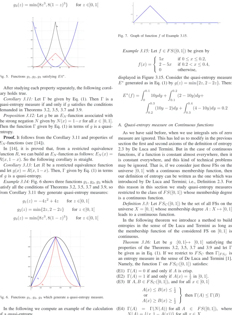
Example 3.10: Figure 5 shows functions g1, g2, g3 which
satisfy property of Theorem 3.9.
g1(z) = 4 (z−0.5)2 for z∈]0,1[ g2(z) = 0 if 0< z≤0.2, z−0.2 if 0.2< z≤0.5, −z+ 0.8 if 0.5< z≤0.8, 0 if 0.8< z <1.
g3(z) = min{8z3,8(1−z)3} forz∈]0,1[
Fig. 5. Functionsg1, g2, g3satisfyingE4∗.
After studying each property separately, the following corol-lary holds true.
Corollary 3.11: Let Γ be given by Eq. (1). Then Γ is a quasi-entropy measure if and only ifgsatisfies the conditions demanded in Theorems 3.2, 3.5, 3.7 and 3.9.
Proposition 3.12: Letgbe anEN-function associated with
the strong negationNgiven byN(x) = 1−xfor allx∈[0,1]. Then the functionΓgiven by Eq. (1) in terms ofgis a quasi-entropy.
Proof. It follows from the Corollary 3.11 and properties of EN-functions (see [14]).
In [14], it is proved that, from a restricted equivalence functionR, we can build anEN-function as follows:EN(x) = R(x,1−x). So the following corollary is straight.
Corollary 3.13: Let R be a restricted equivalence function and letg(x) =R(x,1−x). Then,Γgiven by Eq. (1) in terms of gis a quasi-entropy.
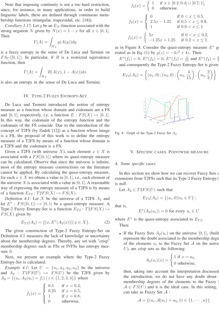
Example 3.14: Fig. 6 shows three functionsg1,g2,g3which
satisfy all the conditions of Theorems 3.2, 3.5, 3.7 and 3.9, so from Corollary 3.11 they generate quasi-entropy measures:
g1(z) =−4z2+ 4z for z∈]0,1[
g2(z) = min{2z,2−2z} for z∈]0,1[
g3(z) = min{8z3,8(1−z)3} forz∈]0,1[
Fig. 6. Functionsg1,g2,g3which generate a quasi-entropy measure.
In the following we compute an example of the calculation of a quasi-entropy.
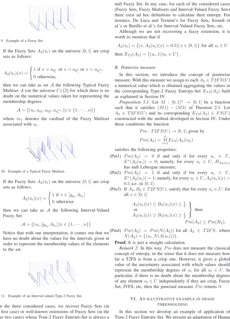
Fig. 7. Graph of functionf of Example 3.15.
Example 3.15: Letf ∈F S([0,1]) be given by
f(x) = 5x if 0≤x≤0.2, 2−5x if 0.2< x≤0.4, 0 otherwise,
displayed in Figure 3.15. Consider the quasi-entropy measure E∗ generated as in Eq. (1) byg(z) = min{2z,2−2z}. Then:
E∗(f) =Z 0.1 0 10ydy+ Z 0.2 0.1 (2−10y)dy+ Z 0.3 0.2 (10y−2)dy+ Z 0.4 0.3 (4−10y)dy= 0.2
A. Quasi-entropy measure on Continuous functions
As we have said before, when we use integrals sets of zero measure are ignored. This has led us to modify in the previous section the first and second axioms of the definition of entropy 2.3 by De Luca and Termini. But in the case of continuous functions, if a function is constant almost everywhere, then it is constant everywhere, and this kind of technical problems may be ignored. That is, if we consider just those FSs on the universe [0,1] with a continuous membership function, then our definition of entropy can be written as the one which was introduced by De Luca and Termini; i.e., Definition 2.3. For this reason in this section we study quasi-entropy measures restricted to the class ofF S([0,1])whose membership degree is a continuous function.
Definition 3.3: LetF SC([0,1]) be the set of all FSs on the
universeX= [0,1]whose membership degreeA:X 7→[0,1] leads to a continuous function.
In the following theorem we introduce a method to build entropies in the sense of De Luca and Termini as long as the membership function of the considered FS on [0,1] is continuous.
Theorem 3.16: Let be g :]0,1[7→ [0,1] satisfying the properties of the Theorems 3.2, 3.5, 3.7 and 3.9 and let Γ be given as in Eq. (1). If we restrict to F SC then Γ|F SC is
an entropy measure in the sense of De Luca and Termini [1]. Namely, the functionΓ onF SC([0,1]) satisfies:
(E1) Γ(A) = 0if and only if Ais crisp.
(E2) Γ(A) = 1if and only if A(x) = 12 in[0,1]. (E3) If A, B∈F SC([0,1]), and for all x∈[0,1]
A(x)≤B(x)≤ 1 2 or A(x)≥B(x)≥ 1 2 thenΓ(A)≤Γ(B)
(E4) Γ(A) = Γ(N(A))for allA ∈ F S([0,1]), where N(A) ={(x,1−A(x))} for allx∈X.
Note that imposing continuity is not a too hard restriction, since, for instance, in many applications, in order to build linguistic labels, these are defined through continuous mem-bership functions (triangular, trapezoidal, etc. [18]).
Corollary 3.17: Letgbe anEN-function associated with the
strong negationN given byN(x) = 1−xfor allx∈[0,1]. Then
Γ(A) = Z
HA
g(A(y))dy
is a fuzzy entropy in the sense of De Luca and Termini on F SC([0,1]). In particular, if R is a restricted equivalence
function, then Γ(A) =
Z
HA
R(A(x),1−A(x))dx is also an entropy in the sense of De Luca and Termini.
IV. TYPE-2 FUZZYENTROPY-SET
De Luca and Termini introduced the notion of entropy measure as a function whose domain and codomain are a FS and [0,1], respectively, i.e. a functionE : F S(X) 7→ [0,1]. In this way, the codomain of the entropy function and the codomain of the FS coincide. Due to the introduction of the concept of T2FS (by Zadeh [12]) as a function whose image is a FS, the proposal of this work is to define the entropy measure of a T2FS by means of a function whose domain is a T2FS and the codomain is a FS.
Given a T2FS (with universe X), each element x∈ X is associated with aF S([0,1])where its quasi-entropy measure can be calculated. Observe that since the universe is infinite, most of the entropy measure constructions on the literature cannot be applied. By calculating the quasi-entropy measure, for eachx∈Xwe obtain a value in[0,1], i.e., each element of the universeXis associated with a value in[0,1]. A reasonable way of expressing the entropy measure of a T2FS is by means of a functionET2:T2F S(X)7→F S(X).
Definition 4.1: Let X be the universe of a T2FS A2 and
let E∗ : F S([0,1]) 7→ [0,1] be a quasi-entropy measure. A
Type-2 Fuzzy Entropy-Set is a function ET2:T2F S(X)7→
F S(X)given by
ET2(A2) ={(x, E∗(A2(x)))|x∈X}. (2)
The given construction of Type-2 Fuzzy Entropy-Set on Definition 4.1 measures the lack of knowledge or uncertainty about the membership degrees. Thereby, any set with "crisp" membership degrees such as FSs or IVFSs has entropy mea-sure0.
Next, we present an example where the Type-2 Fuzzy Entropy-Set is calculated.
Example 4.1: Let U = {u1, u2, u3, u4} be the universe
and A2 : T2F S(U) 7→ F S(U) be the T2FS given by
A2={(ui, A2(ui) =fi)|i∈ {1,2,3,4}} where f1(x) = 0.5 ifx= 0.3, 0.25 ifx= 0.5, 1 ifx= 0.8, 0 otherwise. f2(x) = 1 ifx∈[0.2; 0.4]∪[0.7; 1[, 0 otherwise. f3(x) = 0 if 0< x≤0.5, 2.5x−1.25 if 0.5< x≤0.9, 1 if 0.9< x≤1 f4(x) = 5x if0< x≤0.2, −1.25x+ 1.25 if0.2< x≤1.
as in Figure 8. Consider the quasi-entropy measure E∗
gen-erated as in Eq. (1) by g(z) =−4z2+ 4z. Then:
E∗(f
1) = 0,E∗(f2) = 0,E∗(f3) =154 andE∗(f4) = 23,
and consequently the Type-2 Fuzzy Entropy-Set is given by ET2(A2) = (u1,0),(u2,0), u3, 4 15 , u4, 2 3
Fig. 8. Graph of the Type-2 Fuzzy SetA2.
V. SPECIFIC CASES. POINTWISE MEASURE
A. Some specific cases
In this section we show how we can recover Fuzzy Sets and extensions from T2FSs such that its Type-2 Fuzzy Entropy-Set is null.
Let A2∈T2F S(U)such that
ET2(A2) ={(ui,0)|ui∈U};
that is,
E∗(A2(ui)) = 0 for everyui∈U
where E∗ is the quasi-entropy associated to E
T2.
Then:
• If the Fuzzy SetsA2(ui)on the universe[0,1], (built to
represent the doubt associated to the membership degrees of the elements ui to the Fuzzy Set A on the universe U), are crisp sets as the following:
A2(ui)(x) =
(
1 ifx=a0i
0 otherwise,
then, taking into account the interpretation discussed in the introduction, we do not have any doubt about the membership degrees of the elements to the Fuzzy Set A ∈ F S(U) and it is the ideal case. In this setting, we can take as Fuzzy Set A:
Fig. 9. Example of a Fuzzy Set.
• If the Fuzzy SetsA2(ui)on the universe [0,1]are crisp
sets as follows: A2(ui)(x) = ( 1 if x=a01 i orx=a02i or x=a0mii 0 otherwise,
then we can take as set A the following Typical Fuzzy MultisetA(on the universeU) [2] for which there is no doubt on the numerical values taken for representing the membership degrees: A={(ui, a01 i, a0 2 i, a0 mi i )|i∈ {1,· · ·, n}}
where m1 denotes the cardinal of the Fuzzy Multiset
associated withui.
Fig. 10. Example of a Typical Fuzzy Multiset.
• If the Fuzzy SetsA2(ui)on the universe [0,1]are crisp
sets as follows: A2(ui)(x) =
(
1 ifx∈[a0i, a0i]
0 otherwise
then we can take as A the following Interval-Valued Fuzzy Set:
A={(ui,[a0i, a0i])|i∈ {1,· · ·, n}}
Notice that with our interpretation, it comes out that we have no doubt about the values for the intervals given in order to represent the membership values of the elements to the set.
Fig. 11. Example of an Interval-valued Type-2 Fuzzy Set.
In the three considered cases, we recover Fuzzy Sets (in the first case) or well-known extensions of Fuzzy Sets (in the other two cases) whose Type-2 Fuzzy Entropy-Set is always a
null Fuzzy Set. In any case, for each of the considered cases (Fuzzy Sets, Fuzzy Multisets and Interval-Valued Fuzzy Sets) there exist ad hoc definitions to calculate their entropy. For instance, De Luca and Termini’s for Fuzzy Sets, Szmidt et al.’s or Burillo et al.’s for Interval-Valued Fuzzy Sets, etc.
Although we are not recovering a fuzzy extension, it is worth to mention that if
A2(ui) ={(x, A2(ui)(x) = 0.5)|x∈[0,1]}for allui∈U
thenET2(A2) ={(ui,1)|ui∈U}.
B. Pointwise measure
In this section, we introduce the concept of pointwise measure. With this measure we assign to eachA2∈T2F S(U)
a numerical value which is obtained aggregating the values in the corresponding Type-2 Fuzzy Entropy-Set ET2(A2) built
as explained in Section IV.
Proposition 5.1: Let M : [0,1]n → [0,1] be a function
such that it satisfies (M1) − (M3) of Theorem 2.1. Let A2 ∈ T2F S(U) and its corresponding ET2(A2) ∈ F S(U)
constructed with the method developed in Section IV. Under these conditions the function
P m:T2F S(U)→[0,1]given by P m(A2) =
n M
i=1ET2(A2)(ui)
satisfies the following properties:
(Pm1) P m(A2) = 0 if and only if for every ui ∈ U, E∗(A
2(ui)) = 0; namely, for every ui ∈ U, HA2(ui)
has null Lebesgue measure;
(Pm2) P m(A2) = 1 if and only if for every ui ∈ U, E∗(A
2(ui)) = 1; namely, for everyui∈U,A2(ui)(x) =
0.5 a.e. in[0,1];
(Pm3) IfA2, B2∈T2F S(U), satisfy that for everyui∈U: for
all x∈[0,1] A2(ui)(x)≤B2(ui)(x)≤12 or A2(ui)(x)≥B2(ui)(x)≥12 then P m(A2)≤P m(B2);
(Pm4) P m(A2) = P m(N(A2))for allA2 ∈ T2F S, where
N(A2) ={(ui, N(A(ui)))}.
Proof. It is just a straight calculation.
Remark 2: In this way,P mdoes not measure the classical concept of entropy, in the sense that it does not measure how far a T2FS is from a crisp one. However, it gives a global value of the uncertainty associated with which values should represent the membership degrees of ui for all ui ∈ U. In
particular, if there is no doubt about the membership degrees of any element ui∈U independently if they are crisp, Fuzzy
Set, IVFS, etc, then the punctual measureP mreturns 0. VI. AN ILLUSTRATIVE EXAMPLE IN IMAGE
THRESHOLDING
In this section we develop an example of application of Type-2 Fuzzy Entropy-Set. We present an adaptation of Huang
and Wang’s method [7] to segment images in grayscale. To do so, we build a T2FS associated with the image and we calculate its Type-2 Fuzzy Entropy-Set.
Image segmentation consists of dividing an image into regions (objects) that compound it [19]. More specifically, it consists of assigning a label to each pixel of the image, so that all the pixels which share certain properties have the same label. One of the most used techniques in image segmentation is thresholding or segmentation by gray levels [20], [21], [22]. It is based on the assumption that the objects of the image are only characterized by the intensity of their pixels. When the image has only two objects (called object and background), this thresholding technique consists of finding an intensity value (t) to be considered the threshold. Using that value, we label all the pixels whose intensities are lower or equal thant as background and all the pixels whose intensities are greater than t as object (or vice versa). When there are more than two objects in the image, we need more thresholds, in such a way that all the pixels whose intensities are between two consecutive thresholds belong to the same object.
The results of thresholding are limited when comparing with other segmentation techniques, because the single char-acteristic they take into account is the intensity of every pixel. However, its advantages are the simplicity and low computational cost. This is why this procedure is commonly used as a first step of more complex segmentation algorithms. We consider an image as a set of elements arranged in N rows and M columns. Each element of a grayscale image has a value of intensityqbetween0andL−1(usuallyL= 256). However, we work with normalized images Lq−1 in such a way that q∈[0,1].
As we have said in the introduction, we rewrite Huang and Wang’s algorithm [7] using T2FSs and Type-2 Fuzzy Entropy-Sets (see Algorithm 1).
Algorithm 1 Thresholding algorithm INPUT: Image to segment
OUTPUT: tthe best threshold
1: {Construction of the T2FS}
2: for each intensity levelt∈ {0,1/255, . . . ,254/255}(For every possible threshold) do
3: Construct a FS on the universe [0,1] associated with the intensity levelt
4: end for
5: Calculate the Type-2 Fuzzy Entropy-Set of the resulting T2FS
6: Select as best threshold t the one associated with the lowest element in the Type-2 Fuzzy Entropy-Set
The main idea of this procedure consists in creating a T2FS associated with the image and calculating its entropy set. One of the most difficult tasks is the construction of the T2FS. It should represent the information of how would be the image if we segment it with every possible threshold. For this purpose, we start by fixing the referential set of the T2FS as the set of all possible thresholds in the image: U = {0/255,1/255, . . . ,254/255} (remember the image is normalized). For every element inU, its membership degree
Fig. 12. Example of a Type-2 Fuzzy Set.
is given by a Fuzzy Set. This set has a continuous referential set from 0 to 1. In Figure 12 we show a T2FS that fulfills our conditions.
Each of these functions represents, for a fixed threshold, the membership degree of every possible intensity either to the object or to the background. To construct each of these sets, following [8], we start by calculating the average intensity of the pixels lower or equal than the studied threshold (denoted as mB(t)) and the average intensity of the pixels greater than
the studied threshold (denoted asmO(t)).
The membership function quantifies how close is every posible value (q) to the average of the background or to the average of the object, by means of restricted equivalence functions: A(ui)(q) = ( R(q, mB(ui)) if q≤ui R(q, mO(ui)) if q > ui. (3) We linearly interpolate between every pair of consecutive points (qi,(A(ui)(qi))) and (qi+1,(A(ui)(qi+1))) with i ∈
{0,· · ·,254}. That is, we take the points (0,A(ui)(0)) and
(1/255,A(ui)(1/255))and, for eachs∈[0,1/255], we define
its membership as:
A2(s) = 255(A(ui)(1/255)− A(ui)(0))s+A(ui)(0).
Next, we repeat this procedure for each interval[j/255,(j+ 1)/255], (j = 0, . . . ,254), calculating in each case the equation of the line which passes through the points (j/255,A(ui)(j/255))and((j+1)/255,A(ui)((j+1)/255)).
In this way, we get a continuous membership function de-fined over the whole universe[0,1]. This membership function is piecewise linear and it has only two points where its value is 1: the average of the background (mB(t)) and the average
of the object (mO(t)).
To select the best threshold from the T2FS we use its Type-2 Fuzzy Entropy-Set. We are looking for the threshold whose membership function is as higher as possible for all the pixels in the image. The entropy is minimum when the membership is 0 or 1, and maximum in the middle point. To adapt this concept to our problem, we scale our membership function to [0.5,1], in such a way that the minimum entropy is only achieved when the membership degree is 1.
With our membership construction, the calculation of our entropies is simple, since we can divide the area in 255 trapezoids and we just need to sum the entropy measure of each of these parts multiplied by the proportion of pixels with that intensity. That is, we calculate the entropy of each FS as
E(A2(ui)) =
R
g(A2(ui)(x))dx where A2(ui) is the FS
as-sociated withuion the universe[0,1]andg(x) =R(x,1−x).
In this way we obtain a set of entropies, each one associated with an element of the universe (possible thresholds based on our construction) and we can build the Type-2 Fuzzy Entropy-Set. Finally, we select as the best threshold, the one associated with the lowest entropy measure.
With an illustrative aim, we use this algorithm for thresh-olding the image in Figure 13.
Fig. 13. Original image to segment.
After constructing the T2FS for this image, we useg(x) = R(x,1−x) = 1− |2x−1|to get its associated Type-2 Fuzzy Entropy-Set. The resulting set is as follows:
ET2={(u0,0.6014),(u1,0.6010),(u2,0.6004), . . . ,(u254,0.5935)}
For a better visualization of this set, in Figure 14 we show it graphically. 0 50 100 150 200 250 0.1 0.2 0.3 0.4 0.5 0.6 0.7 0.8
Fig. 14. Fuzzy Entropy-Set for thresholding the image of Figure 13.
The minimum of this Type-2 Fuzzy Entropy-Set corre-sponds to the element (u143,0.1467). So the threshold used
to segment the image is 143/255 and we get the image shown in Figure 15.
Fig. 15. Image of Figure 13 segmented with threshold 143.
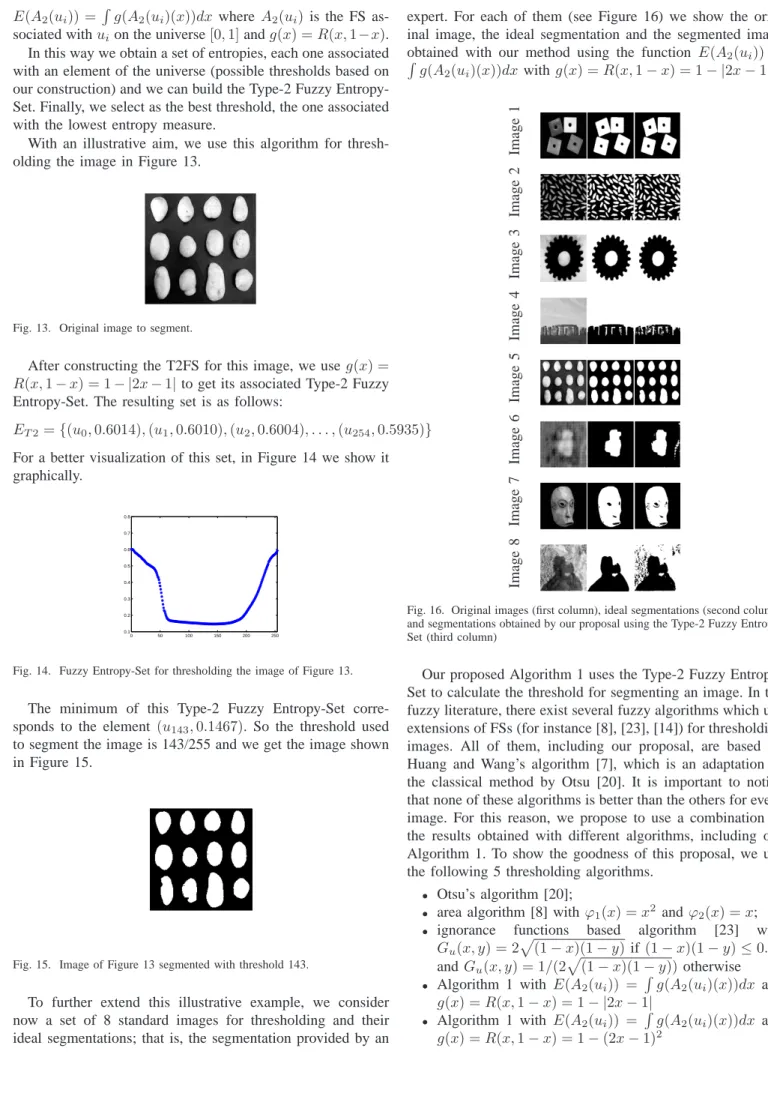
To further extend this illustrative example, we consider now a set of 8 standard images for thresholding and their ideal segmentations; that is, the segmentation provided by an
expert. For each of them (see Figure 16) we show the orig-inal image, the ideal segmentation and the segmented image obtained with our method using the function E(A2(ui)) =
R g(A2(ui)(x))dx withg(x) =R(x,1−x) = 1− |2x−1|. Im ag e 1 Im ag e 2 Im ag e 3 Im ag e 4 Im ag e 5 Im ag e 6 Im ag e 7 Im ag e 8
Fig. 16. Original images (first column), ideal segmentations (second column) and segmentations obtained by our proposal using the Type-2 Fuzzy Entropy-Set (third column)
Our proposed Algorithm 1 uses the Type-2 Fuzzy Entropy-Set to calculate the threshold for segmenting an image. In the fuzzy literature, there exist several fuzzy algorithms which use extensions of FSs (for instance [8], [23], [14]) for thresholding images. All of them, including our proposal, are based on Huang and Wang’s algorithm [7], which is an adaptation of the classical method by Otsu [20]. It is important to notice that none of these algorithms is better than the others for every image. For this reason, we propose to use a combination of the results obtained with different algorithms, including our Algorithm 1. To show the goodness of this proposal, we use the following 5 thresholding algorithms.
• Otsu’s algorithm [20];
• area algorithm [8] withϕ1(x) =x2 andϕ2(x) =x;
• ignorance functions based algorithm [23] with Gu(x, y) = 2 p (1−x)(1−y)if (1−x)(1−y)≤0.25 andGu(x, y) = 1/(2 p (1−x)(1−y))otherwise
• Algorithm 1 with E(A2(ui)) = Rg(A2(ui)(x))dx and g(x) =R(x,1−x) = 1− |2x−1|
• Algorithm 1 with E(A2(ui)) =
R
g(A2(ui)(x))dx and g(x) =R(x,1−x) = 1−(2x−1)2
In Table I we study the obtained thresholds as well as the percentage of pixels correctly segmented with respect to the ideal segmentation for each of the algorithms and each of the 8 images shown in Figure 16. For the sake of simplicity, thresholds have been multiplied by 255. Moreover, we consider the combination of all the obtained thresholds using the arithmetic mean and we also calculate for the latter the percentage of well segmented pixels.
As we can see in Table I, it does not exist one single method which is the best for every possible image. However, when we take the mean of several methods we get good results, which are even the best ones for 4 of the 8 images. So, after combining the results of several algorithms (including Algorithm 1), we see that the obtained segmentations are very good. These segmentations can be taken as a first step in the calculation of segmentations which take into account more properties of the images, apart from the intensity of the pixels.
VII. CONCLUSIONS ANDFUTUREWORK
The construction of entropy measures for Fuzzy Sets with infinite universes results intricate. In this direction one of the main novelties of this study is the introduction of the concept of quasi-entropy. Defined slightly different than the fuzzy entropy given by De Luca and Termini it is proven that both concepts are equivalent if we restrict to continuous membership functions. The quasi-entropy measure has been applied to a T2FS (whose membership degree for an element x in the universe X is a F S([0,1])), generating the novel concepts of Type-2 Fuzzy Entropy-Set and pointwise measure. Finally, we have shown the usefulness of the Type-2 Fuzzy Entropy-Set in an illustrative example in Huang and Wang’s algorithm for image thresholding.
Due to the relevance of a theoretical method to calculate the entropy of T2FSs we leave for a future work the deeper study of the application, i.e. we leave for future work the deep analysis of the conditions under which the algorithms consid-ered in the illustrative example (Algorithm 1) can improve the thresholds usually calculated.
APPENDIX
PROOFS OF THETHEOREMS
Theorem 3.2 LetΓ :F S([0,1])7→[0,1]be a function given by Eq. (1). Then
Γsatisfies (E1∗)if and only if g(z)6= 0for all z∈]0,1[.
Proof.
⇒)LetΓ satisfy(E1∗).
Suppose that g(z0) = 0 for some z0 ∈ ]0,1[. Let A ∈
F S([0,1]) be given by A(z) = z0 for all z ∈ [0,1]. Then,
Γ(A) = R
HAg(A(y))dy =
R1
0 g(z0) = 0 and Γ does not
satisfy(E1∗).
⇐)Takeg(z)6= 0for all z∈]0,1[.
• If HA has Lebesgue measure 0 then Γ(A) =
R
HAg(A(y))dy= 0.
• If Γ(A) = R
HAg(A(y))dy = 0, since g(z) 6= 0 for
all z ∈ ]0,1[, then g(A(y)) 6= 0 for all y ∈ HA.
Consequently,Γ(A) =R
HAg(A(y))dy= 0can only hold
if m(HA) = 0 . Thus,Γ satisfies (E1∗).
Theorem 3.5 LetΓ :F S([0,1])7→[0,1]be a function given by Eq. (1). Then,
Γsatisfies (E2∗)if and only if g−1(1) = 1
2
Proof.
⇒)Let Γsatisfy (E2∗).
• Suppose thatg(12)6= 1. Let the FSAbe given byA(x) =
1
2 for all x ∈ [0,1]. Then Γ(A) =
R HAg(A(y))dy = R1 0 g( 1 2) = g( 1
2) 6= 1, which is in contradiction with
(E2∗).
• Suppose g(z0) = 1 for some z0 6= 12. Given A(x) =z0
for all x ∈ [0,1] we have Γ(A) = R
HAg(A(y))dy =
R1
0 g(z0) =g(z0) = 1, which is again in contradiction
with(E2∗). ⇐)Let g satisfyg−1(1) ={1 2}. • If A(x) = 1 2 a.e. in [0,1], then m({x ∈HA | A(x)6= 1 2}) ≤ m({x | A(x) 6= 1 2}) = 0 and m({x | A(x) = 1 2)}) = 1. Thus, Γ(A) = R HAg(A(y))dy = R {x∈HA|A(x)=6 12}g(A(y))dy+ R {x|A(x)=1 2}g(A(y))dy = 0 +R {x|A(x)=1 2}g( 1 2)dy=g( 1 2) = 1. • Now take Γ(A) =R HAg(A(y))dy= 1.
Sincem(HA)≤1andg(z)≤1thenΓ(A) = 1can only hold if m(HA) = 1 and g(A(y)) = 1 for all y ∈ HA. But giveny∈HA,g(A(y)) = 1only ifA(y) =12. Since the measure of HA is 1, this means that A = 12 a.e. in
[0,1].
Consequently, Γsatisfies (E2∗).
Theorem 3.7 LetΓ :F S([0,1])7→[0,1]be a function given by Eq. (1). Then,Γsatisfies(E3∗)if and only ifgis increasing
on 0,1 2 and decreasing on1 2,1 . Proof. ⇒)Let Γsatisfy (E3∗).
1) Suppose g is not increasing in ]0,12]. Then, there exist z1, z2 such that0< z1< z2≤21 and g(z1)> g(z2).
LetA(x) =z1 for allx∈[0,1]and B(x) =z2 for all
x∈[0,1]. AsA(x)≤B(x)≤ 12 for all x∈[0,1], by (E3∗)it must be satisfied thatΓ(A)≤Γ(B).
ButΓ(A) =R HAg(A(y))dy= R1 0 g(z1)dy=g(z1)and Γ(B) =R HBg(B(y))dy= R1 0 g(z2)dy =g(z2), which is in contradiction withg(z1)> g(z2).
2) Suppose that g is not decreasing in[1
2,1[. Then, there
exist z1, z2 such that 12 ≤ z1 < z2 <1 and g(z1) <
g(z2).
LetA(x) =z2 for allx∈[0,1]and B(x) =z1 for all
x∈[0,1]. Since 12 ≤B(x)≤A(x) for all x∈[0,1], by(E3∗) Γ(A)≤Γ(B)must be satisfied. ButΓ(A) =R HAg(A(y))dy= R1 0 g(z2)dy=g(z2)and Γ(B) =R HBg(B(y))dy= R1 0 g(z1)dy =g(z1), which is in contradiction withg(z1)< g(z2).
Otsu Area Ignorance Alg1v1 Alg1v2 Average u % u % u % u % u % u % Im. 1 79 93.6614 50 97.3064 13 96.6738 50 97.3064 29 97.2375 44 97.4059 Im. 2 74 92.2227 56 92.7227 11 90.8861 58 92.7074 47 92.7099 49 92.7762 Im. 3 104 98.0148 87 98.2887 13 97.6454 96 98.1731 88 98.2887 77 98.3741 Im. 4 136 95.8283 135 95.7278 135 95.7278 135 95.7278 134 95.5912 135 95.7278 Im. 5 127 95.8474 140 95.9545 177 93.3757 143 95.9621 157 95.2479 148 95.7224 Im. 6 134 95.6408 138 96.4085 97 64.4245 138 96.4085 141 96.7835 129 94.9316 Im. 7 71 95.9748 50 96.6721 3 92.2469 52 96.6337 49 96.7208 45 96.8029 Im. 8 123 89.0935 121 89.5726 121 89.5726 121 89.5726 121 89.5726 121 89.5726 TABLE I
THRESHOLDS(MULTIPLIED BY255)AND PERCENTAGE OF WELL CLASSIFIED PIXELS. (OTSU) RESULTS OBTAINED WITHOTSU’S METHOD. (AREA) RESULTS OBTAINED AREA ALGORITHM ANDϕ1(x) =x2ANDϕ2(x) =x. (IGNORANCE) RESULTS OBTAINED WITH WITH THE ALGORITHM BASED ON
THE IGNORANCE ANDGu(x, y) = 2 p
(1−x)(1−y)IF(1−x)(1−y)≤0.25ANDGu(x, y) = 1/(2
p
(1−x)(1−y))OTHERWISE. (ALG2V1) RESULTS OBTAINED WITH OUR PROPOSAL,USINGE=R
g(A(x))dxWITHg(x) =R(x,1−x) = 1− |2x−1|. (ALG2V2) RESULTS OBTAINED WITH
OUR PROPOSAL,USINGE=R
g(A(x))dxWITHg(x) =R(x,1−x) = 1−(2x−1)2
.
First of all, notice thatg has a maximum on 12.
Suppose thatA, B∈F S([0,1])satisfy that for allx∈[0,1] A(x)≤B(x)≤12 or A(x)≥B(x)≥12 (4)
and let us see thatE∗(A)≤E∗(B).
First, we proveHA⊆HB. Takex∈HA, by the Definition ofHA thenA(x)= 06 andA(x)6= 1. There are three different cases: • If A(x) < 12 then 0 < A(x) ≤ B(x) ≤ 12, so 0 < B(x)<1 andx∈HB. • If A(x) > 12 then 1 > A(x) ≥ B(x) ≥ 12, so 0 < B(x)<1 andx∈HB. • IfA(x) =12 then 12 ≤B(x)≤ 12, so0< B(x) =12 <1 and x∈HB. Thus,HA⊆HB. Thereby, Γ(A) = Z HA g(A(y))dy≤ Z HB g(A(y))dy = Z {x|0<B(x)<1 2} g(A(y))dy+ Z {x|B(x)=1 2} g(A(y))dy + Z {x|1 2<B(x)<1} g(A(y))dy≤ Z {x|0<B(x)<1 2} g(B(y))dy + Z {x|B(x)=1 2} g(B(y))dy+ Z {x|1 2<B(x)<1} g(B(y))dy = Z HB g(B(y))dy= Γ(B) where the first inequality holds due to HA ⊆ HB and the second one because g is an increasing function on ]0,1
2],
becauseg has a maximum on 12 and becausegis decreasing on[12,1[, respectively.
Theorem 3.9 LetΓ :F S([0,1])7→[0,1]be a function given by Eq. (1). Then,
Γ satisfies(E4∗)if and only if g is a symmetric function
with respect toz= 1
2, i.e.,g(z) =g(1−z)for all z∈]0,1[.
Proof. First of all, notice that HN(A) ={x|N(A(x)) ∈
]0,1[}={x|1−A(x)∈]0,1[}={x|A(x)∈]0,1[}=HA.
⇒)Let Γsatisfy (E4∗).
Suppose thatgis not symmetric, then there existsz0∈]0,1[
such that g(z0)6=g(1−z0). LetA(x) =z0 for allx∈[0,1],
then N(A(x)) = 1−z0 for allx∈[0,1]. However, function
Γ yields Γ(A) =R HAg(A(y))dy= R1 0 g(z0)dy=g(z0)and Γ(N(A)) = Z HN(A) g(N(A(y)))dy = Z HN(A) g(1−z0)dy=g(1−z0),
which is in contradiction with (E4∗).
⇐)Let g be a symmetric function with respect toz=12. Then Γ(A) = Z HA g(A(y))dy = Z HN(A) g(A(y))dy= Z HN(A) g(1−A(y))dy = Z HN(A) g(N(A(y)))dy= Γ(N(A))
where the second equality holds becauseHA=HN(A), the
third one holds because gis symmetric and the fourth one by the expression of negation.
REFERENCES
[1] A. D. Luca and S. Termini, “A definition of a nonprobabilistic entropy in the setting of fuzzy sets theory,” Information and Control, vol. 20, no. 4, pp. 301 – 312, 1972.
[2] H. Bustince, E. Barrenechea, M. Pagola, J. Fernandez, Z. Xu, B. Bedre-gal, J. Montero, H. Hagras, F. Herrera, and B. De Baets, “A historical account of types of fuzzy sets and their relationships,” Fuzzy Systems,
IEEE Transactions on, vol. PP, no. 99, pp. 1–1, 2015.
[3] E. Szmidt and J. Kacprzyk, “Entropy for intuitionistic fuzzy sets,” Fuzzy
Sets and Systems, vol. 118, no. 3, pp. 467 – 477, 2001.
[4] P. Burillo and H. Bustince, “Entropy on intuitionistic fuzzy sets and on interval-valued fuzzy sets,” Fuzzy Sets and Systems, vol. 78, no. 3, pp. 305 – 316, 1996.
[5] N. Pal, H. Bustince, M. Pagola, U. Mukherjee, D. Goswami, and G. Beliakov, “Uncertainties with Atanassov’s intuitionistic fuzzy sets: Fuzziness and lack of knowledge,” Information Sciences, vol. 228, pp. 61 – 74, 2013.
[6] L. A. Zadeh, “Quantitative fuzzy semantics,” Inform. Sci., no. 3, pp. 159 – 176, 1971.
[7] L.-K. Huang and M.-J. J. Wang, “Image thresholding by minimizing the measures of fuzziness,” Pattern Recognition, vol. 28, no. 1, pp. 41 – 51, 1995.
[8] H. Bustince, E. Barrenechea, and M. Pagola, “Image thresholding using restricted equivalence functions and maximizing the measures of similarity,” Fuzzy Sets and Systems, vol. 158, no. 5, pp. 496 – 516, 2007.
[9] P. Melo-Pinto, P. Couto, H. Bustince, E. Barrenechea, M. Pagola, and J. Fernandez, “Image segmentation using atanassov’s intuitionistic fuzzy sets,” Expert Systems with Applications, vol. 40, no. 1, pp. 15–26, Jan 2013.
[10] G. Beliakov, M. Pagola, and T. Wilkin, “Vector valued similarity measures for Atanassov’s intuitionistic fuzzy sets,” Information Sciences, vol. 208, pp. 352–367, 2014.
[11] L. Zadeh, “Fuzzy sets,” Information and Control, vol. 8, no. 3, pp. 338 – 353, 1965.
[12] ——, “The concept of a linguistic variable and its application to approximate reasoning I,” Information Sciences, vol. 8, no. 3, pp. 199 – 249, 1975.
[13] D. Dubois, W. Ostasiewicz, and H. Prade, “Fuzzy sets: History and basic notions,” in Fundamentals of Fuzzy Sets, ser. The Handbooks of Fuzzy Sets Series, D. Dubois and H. Prade, Eds. Springer US, 2000, vol. 7, pp. 21–124.
[14] H. Bustince, E. Barrenechea, and M. Pagola, “Relationship between restricted dissimilarity functions, restricted equivalence functions and normal en-functions: Image thresholding invariant,” Pattern Recognition
Letters, vol. 29, no. 4, pp. 525 – 536, 2008.
[15] L. Xuecheng, “Entropy, distance measure and similarity measure of fuzzy sets and their relations,” Fuzzy Sets and Systems, vol. 52, no. 3, pp. 305 – 318, 1992.
[16] R. Yager, “Entropy measures under similarity relations,” International
J. General Systems, no. 20, pp. 341 – 358, 1992.
[17] H. Bustince, E. Barrenechea, and M. Pagola, “Restricted equivalence functions,” Fuzzy Sets and Systems, vol. 157, no. 17, pp. 2333 – 2346, 2006.
[18] J. Sanz, A. Fernandez, H. Bustince, and F. Herrera, “Ivturs: A linguistic fuzzy rule-based classification system based on a new interval-valued fuzzy reasoning method with tuning and rule selection,” IEEE
Transac-tions on Fuzzy Systems, vol. 21, pp. 399–411, 2013.
[19] K. Fu and J. Mui, “A survey on image segmentation,” Pattern
Recog-nition, vol. 13, no. 1, pp. 3 – 16, 1981.
[20] N. Otsu, “A threshold selection method from gray-level histograms,”
Systems, Man and Cybernetics, IEEE Transactions on, vol. 9, no. 1, pp.
62–66, Jan 1979.
[21] P. K. Sahoo, S. Soltani, A. K. Wong, and Y. C. Chen, “A survey of thresholding techniques,” Comput. Vision Graph. Image Process., vol. 41, no. 2, pp. 233–260, Feb. 1988.
[22] M. Sezgin and B. Sankur, “Survey over image thresholding techniques and quantitative performance evaluation,” Journal of Electronic
Imag-ing, 2004.
[23] H. Bustince, M. Pagola, E. Barrenechea, J. Fernandez, P. Melo-Pinto, P. Couto, H. Tizhoosh, and J. Montero, “Ignorance functions. an application to the calculation of the threshold in prostate ultrasound images,” Fuzzy Sets and Systems, vol. 161, pp. 20 – 36, 2010.
Laura De Miguel received the degree in mathemat-ics from the University of Zaragoza, Spain, in 2012. She is currently a Phd student in the Department of Automatics and Computation, Public University of Navarra. Her areas of interest are fuzzy logics and their generalizations related with concepts such as aggregation functions.
Helida Santos received the M.Sc. degree in Systems and Computing from the Federal University of Rio Grande do Norte (UFRN), Natal, Brazil, in 2008. She is currently a Phd student in the Program of Graduate Studies in Systems and Computing, PPgSC/UFRN. Her research interests include: non-standard fuzzy sets theory, aggregation functions and fuzzy measures.
Mikel Sesma-Sara received the M.Sc. degree in mathematics from the University of Zaragoza in 2015. He is currently a Ph.D. student in the Depart-ment of Automatics and Computation, Public Uni-versity of Navarra, Pamplona, Spain. His research interests are aggregation and fusion functions, fuzzy sets theory and extensions of fuzzy sets.
Benjamin Bedregal received the Ph.D. degree in computer sciences from the Federal University of Pernambuco (UFPE), Recife, Brazil, in 1996. In 1996, he became Assistant Professor at the Depart-ment of Informatics and Applied Mathematics, Fed-eral University of Rio Grande do Norte (UFRN), Na-tal, Brazil, where he is currently a Full Professor. His research interests include: non-standard fuzzy sets theory, aggregation functions, clustering, decision making, fuzzy mathematics, and fuzzy automata.
Aranzazu Jurio received the M.Sc. and Ph.D. de-grees in Computer Sciences from the Public Univer-sity of Navarra, Pamplona, Spain, in 2008 and 2013 respectively. She is currently an Assistant Professor with the Department of Automatics and Compu-tation, Public University of Navarra. Her research interests are image processing, focusing on zooming and segmentation, and applications of fuzzy sets and their extensions.
Humberto Bustince is full professor of Computer Science and Artificial Intelligence in the Public Uni-versity of Navarra. He is the main researcher of the Artificial Intelligence and Approximate Reasoning group of this University, whose main research lines are both theoretical (aggregation functions, infor-mation and comparison measures, fuzzy sets and extensions) and applied (image processing, classifi-cation, machine learning, data mining and big data). He has led 11 I+D public-funded research projects, at a national and at a regional level. Now he is the main researcher of a project in the Spanish Science Program and of scientific network about fuzzy logic and soft computing. He has been in charge of research projects collaborating with private companies such as Caja de Ahorros de Navarra, INCITA, Gamesa or Tracasa. He has taken part in two international research projects. He has authored more than 200 works, according to Web of Science, in conferences and international journals, with around 100 of them in journals of the first quartile of JCR. Moreover, five of these works are also among the highly cited papers of the last ten years, according to Science Essential Indicators of Web of Science. He has regular collaborations with leading international research groups from countries such as the United Kingdom, Belgium, Australia, Germany, Portugal the Czech Republic, Slovakia, Canada, the United States or Brazil. He is editor-in-chief of the online magazine Mathware&Soft Computing of the European Society for Fuzzy Logic and Technologies (EUSFLAT) and of the Axioms journal. He is associated editor of the IEEE Transactions on Fuzzy Systems journal and member of the editorial board of the journals Fuzzy Sets and Systems, Information Fusion, International Journal of Computational Intelligence Systems and Journal of Intelligent&Fuzzy Systems. He is co-author of a monography about averaging functions and co-editor of several books. He has organized some re-known international conferences such as EUROFUSE 2009 and AGOP 2013. He is Senior member of the IEEE Association and Fellow of the International Fuzzy Systems Association (IFSA).
Hani Hagras (M’03-SM’05,F’13) received the B.Sc. and M.Sc. degrees in electrical engineering from Alexandria University, Alexandria, Egypt, and the Ph.D. degree in computer science from the Uni-versity of Essex, Colchester, U.K. He is a Professor in the School of Computer Science and Electronic Engineering, Director of the Computational Intelli-gence Centre and the Head of the Fuzzy Systems Research Group in the University of Essex, UK. His major research interests are in computational intelligence, notably type-2 fuzzy systems, fuzzy logic, neural networks, genetic algorithms, and evolutionary computation. His research interests also include ambient intelligence, pervasive computing and intelligent buildings. He is also interested in embedded agents, robotics and intelligent control. He has authored more than 300 papers in international journals, conferences and books. He is a Fellow of the Institute of Electrical and Electronics Engineers (IEEE) and he is also a Fellow of the Institution of Engineering and Technology (IET (IEE). He was the Chair of IEEE Computational Intelligence Society (CIS) Senior Members Sub-Committee. His research has won numerous prestigious international awards where most recently he was awarded by the IEEE Computational Intelligence Society (CIS), the 2013 Outstanding Paper Award in the IEEE Transactions on Fuzzy Systems and he was also awarded the 2006 Outstanding Paper Award in the IEEE Transactions on Fuzzy Systems. He is an Associate Editor of the IEEE Transactions on Fuzzy Systems. He is also an Associate Editor of the International Journal of Robotics and Automation, the Journal of Cognitive Computation and the Journal of Ambient Computing and Intelligence. He is a member of the IEEE Computational Intelligence Society (CIS) Fuzzy Systems Technical Committee and IEEE CIS conference committee. Prof. Hagras chaired several international conferences where he will act as the Programme Chair of the 2017 IEEE International Conference on Fuzzy Systems, Naples, Italy, July 2017 and he served as the General Co-Chair of the 2007 IEEE International Conference on Fuzzy systems London.
![Fig. 1. Inclusion relationships of extensions of Fuzzy Sets in [2]](https://thumb-us.123doks.com/thumbv2/123dok_us/10964724.2984702/2.892.64.826.72.1136/fig-inclusion-relationships-extensions-fuzzy-sets.webp)