Clustering-Based Personalization

(1)

Scholarship@Western

Electronic Thesis and Dissertation Repository

September 2015

Clustering-Based Personalization

Seyed Nima Mirbakhsh

The University of Western Ontario

Supervisor

Dr. Charles X. Ling

The University of Western Ontario Graduate Program in Computer Science

A thesis submitted in partial fulfillment of the requirements for the degree in Doctor of Philosophy

Follow this and additional works at: https://ir.lib.uwo.ca/etd

Part of the Artificial Intelligence and Robotics Commons, and the Databases and Information Systems Commons

Recommended Citation Recommended Citation

Mirbakhsh, Seyed Nima, "Clustering-Based Personalization" (2015). Electronic Thesis and Dissertation Repository. 3174.

https://ir.lib.uwo.ca/etd/3174

This Dissertation/Thesis is brought to you for free and open access by Scholarship@Western. It has been accepted for inclusion in Electronic Thesis and Dissertation Repository by an authorized administrator of

(2)

by

(Seyed) Nima Mirbakhsh

Graduate Program in Computer Science

A thesis submitted in partial fulfillment

of the requirements for the degree of

Doctor Of Philosophy

The School of Graduate and Postdoctoral Studies

The University of Western Ontario

London, Ontario, Canada

c

(3)

I would like to express my special thanks to my supervisor Professor Dr. Charles Ling, you have been a great mentor for me. I would like to thank you for encouraging my research and for allowing me to grow as a research scientist. I would also like to thank my committee members, Dr. Veksler, Dr. Huang, Dr. Yu and Dr. Mercer for serving as my committee members. I also want to thank you for your brilliant comments and suggestions. I would especially like to thank everyone at Arcane Inc. for their valuable suggestions and supports.

A special thanks to my precious parents. Words cannot express how grateful I am to them for all of the sacrifices that youve made on my behalf. At the end I would like express appreci-ation to my beloved wife, Nobar, who spent sleepless nights with and was always my support in the moments when there was no one to answer my queries. I love you all dearly.

(4)

Recommendation systems have been the most emerging technology in the last decade as one of

the key parts in e-commerce ecosystem. Businesses offer a wide variety of items and contents through different channels such as Internet, Smart TVs, Digital Screens, etc. The number of these items sometimes goes over millions for some businesses. Therefore, users can have

trouble finding the products that they are looking for. Recommendation systems address this

problem by providing powerful methods which enable users to filter through large information

and product space based on their preferences. Moreover, users have different preferences. Thus, businesses can employ recommendation systems to target more audiences by addressing

them with personalized content. Recent studies show a significant improvement of revenue and

conversion rate for recommendation system adopters.

Accuracy, scalability, comprehensibility, and data sparsity are main challenges in

recom-mendation systems. Businesses need practical and scalable recomrecom-mendation models which

accurately personalize millions of items for millions of users in real-time. They also prefer

comprehensible recommendations to understand how these models target their users. However,

data sparsity and lack of enough data about items, users and their interests prevent

personal-ization models to generate accurate recommendations.

In Chapter 1, we first describe basic definitions in recommendation systems. We then

shortly review our contributions and their importance in this thesis. Then in Chapter 2, we

review the major solutions in this context. Traditional recommendation system methods usually

make a rating matrix based on the observed ratings of users on items. This rating matrix is then

employed in different data mining techniques to predict the unknown rating values based on the known values.

In a novel solution, in Chapter 3, we capture the mean interest of the cluster of users on the

cluster of items in a cluster-level rating matrix. We first cluster users and items separately based

on the known ratings. In a new matrix, we then present the interest of each user clusters on each

item clusters by averaging the ratings of users inside each user cluster on the items belonging

(5)

predict the future cluster-level interests. Our final rating prediction includes an aggregation of

the traditional user-item rating predictions and our cluster-level rating predictions.

Generating personalized recommendation for cold-start users, or users with only few

feed-back, is a big challenge in recommendation systems. Employing any available information

from these users in other domains is crucial to improve their recommendation accuracy. Thus,

in Chapter 4, we extend our proposed clustering-based recommendation model by including

the auxiliary feedback in other domains. In a new cluster-level rating matrix, we capture the

cluster-level interests between the domains to reduce the sparsity of the known ratings. By

factorizing this cross-domain rating matrix, we effectively utilize data from auxiliary domains to achieve better recommendations in the target domain, especially for cold-start users.

In Chapter 5, we apply our proposed clustering-based recommendation system toMorphio

platform used in a local digital marketing agency called Arcane inc.Morphiois an smart

adap-tive web platform, which is designed to help Arcane to produce smart contents and target more

audiences. In Morphio, agencies can define multiple versions of content including texts,

im-ages, colors, and so on for their web pages. A personalization module then matches a version of

content to each user using their profiles. Our ongoing real time experiment shows a significant

improvement of user conversion employing our proposed clustering-based personalization.

Finally, in Chapter 6, we present a summary and conclusions for this thesis. Parts of this

thesis were submitted or published in peer-review journal and conferences including ACM

Transactions on Knowledge Discovery from Data and ACM Conferences on Recommender

Systems.

Keywords: Personalization, recommendation systems, collaborative filtering, content mar-keting, data mining

(6)

Certificate of Examination ii

Acknowlegements ii

Abstract iii

List of Figures vii

List of Tables ix

List of Appendices x

1 Introduction 1

1.1 Recommendation Systems . . . 1

1.2 Personalization . . . 3

1.3 Content Filtering . . . 4

1.4 Collaborative Filtering . . . 4

1.5 Hybrid Techniques . . . 4

1.6 Cross-Domain Recommendations . . . 5

1.7 Evaluation Metrics . . . 6

1.8 Adaptive Web . . . 7

1.9 Contributions of this Thesis . . . 8

2 Literature Review 11 2.0.1 K-Nearest Neighbor (KNN) . . . 11

2.0.2 Matrix Factorization . . . 12

2.0.3 Functional Matrix Factorizations . . . 15

2.0.4 Neighborhood-Aware Models . . . 15

2.0.5 Clustering-Based Recommendations . . . 16

2.0.6 Implicit vs. Explicit Feedback . . . 17

3 Leveraging Clustering to Improve Collaborative Filtering 23 3.1 Introduction . . . 23

3.2 The Proposed Models . . . 24

3.2.1 Clustering-Based Matrix Factorization . . . 27

3.2.2 Employing More Clusters . . . 29

3.2.3 Integrating Cluster-Level Preferences With Various Methods . . . 30

(7)

3.3.2 Comparison Regarding Rating Prediction . . . 36

3.3.3 Cold-Start Users . . . 39

3.3.4 Sub-experiments . . . 42

Different Clustering Methods . . . 42

Employing More Clusters . . . 43

3.4 Complexity . . . 45

3.5 Relation to Previous Work . . . 46

4 Improving Top-N Recommendation for Cold-Start Users via Cross-Domain In-formation 48 4.1 Introduction . . . 48

4.2 The Proposed Method . . . 50

4.2.1 Making A Cross-Domain Coarse Matrix . . . 51

4.2.2 Generating Recommendations . . . 54

4.2.3 Factorizing Matrices Considering Unobserved Ratings . . . 54

4.3 Experiments . . . 56

4.3.1 Performance on All Users . . . 61

4.3.2 Performance on Cold-Start Users . . . 64

4.4 Complexity . . . 67

4.5 Relation To Previous Work . . . 67

5 Clustering-Based Personalization In Adaptive Webs 71 5.1 Introduction . . . 71

5.2 Morphio Platform . . . 73

5.3 Personalization Module . . . 74

5.4 Content Analytic Module . . . 77

5.5 Experiment . . . 79

5.6 Relation to Previous Work . . . 81

6 Summary, and Conclusions 82 Bibliography 86 A Basic Concepts 94 A.1 Clustering . . . 94

Curriculum Vitae 96

(8)

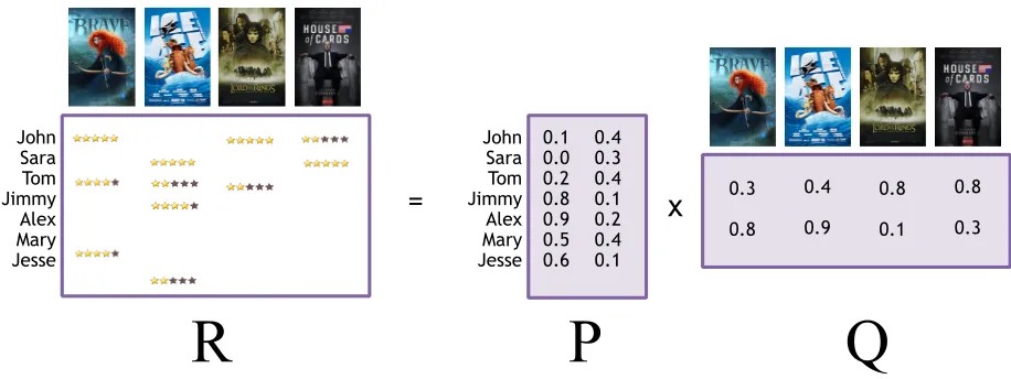
2.1 Factorizing rating matrix R into lower dimension matrices P, and Q, where

R=P.QT. . . 13 2.2 Users watch movies that they think they may like. Hence, a rated movie can be

considered as an interesting movie for a user. . . 18

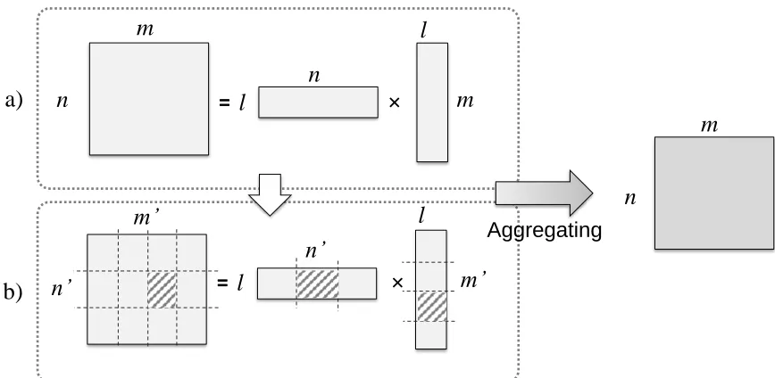
3.1 Factorizing rating matrixRinto latent matricesPandQ(a) and clustering these found latent matrices to produce cluster-level rating matrixRC. (b) Factorizing

rating matrixRC and aggregating these two levels of latent vectors to generate

the recommendations. . . 25 3.2 Clustering latent matrices Pand Q to achieve clusters of users and items and

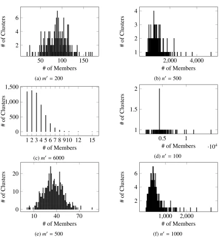
producing the coarse matrix. The coarse matrix generalizes preferences of users into a cluster-level which leads to less sparsity inRc. . . 27 3.3 Distribution of clusters of items and users in different sizes in the Netflix dataset. 35 3.4 The accuracy of the proposed clustering-based models applying on the two

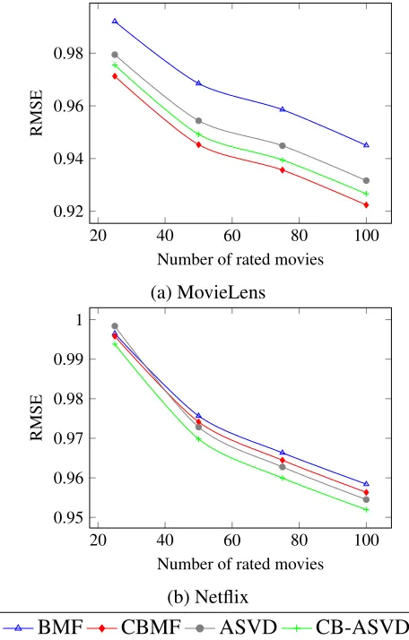
datasets. It shows that our proposed extensions outperform their non-extended models in the both datasets (l= 50 is used to achieve these results). . . 38 3.5 A comparison between Biased Matrix Factorization (BMF) and our proposed

Clustering-based Matrix Factorization (CBMF) for different selection ofl (di-mension of latent vectors). . . 39 3.6 A comparison over the RMSE of the extended and non-extended models for

the cold-start users. . . 41 3.7 Applying different clustering methods in users and items latent spaces in both

datasets and its effect on the CBMF’s result. . . 44 3.8 Applying clustering multiple times with different number of clusters and

em-ploy those found clusters in CBMF model. By emem-ploying more clusters with variety of sizes, rating prediction (RMSE) improves slightly. . . 45

4.1 (Left) Cross-Domain rating matrixRincluding rating matrices of domains Mu-sic and Movies with overlapped users (dashed area). The rating matrix is very sparse as many entries in the top right and lower left are missing values. (Right) Coarse matrixRc _{including mean ratings between cluster of users and cluster}

of items. As shown, the coarse matrix reduces the sparsity ofRby propagating the observed ratings into unobserved ratings. Note that the white area (missing values) is much reduced. . . 53 4.2 Number of observed ratings in different domains in the Amazon dataset. . . 56

(9)

of other five domains are included in the cross-domain methods. . . 58 4.4 Comparing ‘Single-MF’, ‘Collective-MF’, and ‘Cross-CBMF’ for all users in

the 10 selected domains in the Epinions dataset. For each domain, information of other nine domains are included in the cross-domain methods. . . 59 4.5 Comparing the selected methods on cold start users combining all 6 domains

in Amazon dataset. . . 62 4.6 Comparing the selected methods on cold start users combining all 10 domains

in the Epinions dataset. . . 63 4.7 Effect of changing αvalue on aggregated recommendations employing top-N

evaluation (N=20) in Amazon dataset. Note that forα = 0 the recall result is same as ‘Collective-MF’ ’s result. The effect of cluster-level recommendations increases asαincreases. . . 65 4.8 Effect of changing theαvalue on aggregated recommendations employing

top-N evaluation (top-N=20) in Epinions dataset. Note that forα=0 the recall result is same as ‘Collective-MF’ ’s result. The effect of cluster-level recommendations increases asαincreases. . . 66

5.1 A general view on our designed personalization platform. . . 74 5.2 The distribution of audiences versus their number of page visits. . . 79 5.3 Comparing our proposed CBP method with three other methods regarding user

conversion optimization. . . 80

(10)

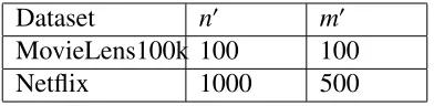
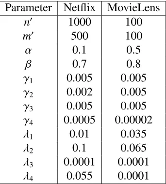
3.1 The final selectedm0 and n0 that is employed in the evaluation of our exten-sion methods. These numbers are found employing a validation set from each dataset, and by trying different selection ofm0 _and_n0_{. . . 34}

3.2 The table shows the movies inside a number of formed clusters in the Netflix dataset. As shown, it seems that movies in same genre and almost similar years of production tend to be in same clusters. Careful analysis shows that about 2/3 of the clusters have some meaningful similarities. . . 37 3.3 RMSE results from applying CBMF with different values for α and β on a

validation set in the MovieLens dataset. . . 38 3.4 Resulting RMSE by applying CBMF with different values of clusters (m0 and

n0) on a validation set in the MovieLens dataset. . . 39 3.5 Employed parameters in Algorithm 3 in the datasets. . . 40

4.1 Number of users, items, and observed ratings in the six selected domains in the Amazon dataset. . . 57 4.2 Percentage of user overlaps between different domains in the Amazon dataset. . 57 5.1 Each web page will be cut into different splits using these frames. . . 78

(11)

Appendix A Basic Concepts . . . 94

(12)

Introduction

In this chapter we review few basic concepts in recommendation systems, and then review our

contributions in this thesis.

1.1 Recommendation Systems

Recommendation systems are key parts of the information and e-commerce ecosystem [11],

where businesses offer an enormous number of items through different channels such as World Wide Web (WWW), Smart TVs, Digital Screens, etc. Therefore, users can have trouble

find-ing the products that they are lookfind-ing for. Recommendation systems address this problem by

providing powerful methods which enable users to filter through large information and product

space based on their preferences. Here are few real world examples of employing

recommen-dation systems in e-commerce:

• Google newsemploys recommendation system to suggest news articles to its users.

• Netflixuses its users’ feedback to recommend them movies that they would like.

In recommendation systems, there are at least two classes of entities; Users and items,

where users have preferences for certain items [41]. The data itself is commonly represented

as a rating matrix or a utility matrixRto show the degree of preference of users on a subset of

items:

(13)

R=                             

i1 i2 . . . im

u1 r11 r12 . . . r1m

u2 r21 r22 . . . r2m

..

. ... ... . .. ...

un rn1 rn2 . . . rnm

                            

whereunrepresents the nth user,imrepresents themth item,nis the number of users,mis

the number of items, andri j represents the rating of userion item j.

We assume that the values are from an ordered set. For instance, integers 1 to 5 represent the

number of stars that the user gave as a rating to a movie in Netflix. In an usual recommendation

scenario, matrixRis sparse. That means we only have few known ratings from each users and

the rest of the ratings are unknown. The goal of recommendation systems is to predict these

unknown values and prepare a list of relevant items for each user. Here are main challenges in

recommendations systems:

• Accuracy: Businesses employ recommendations to first help users by finding their

re-lated items, and second, to increase their own revenue. Accuracy of recommendations

plays a major role to achieve both these goals.

• Scalability: Recommendation systems need to handle millions of users and millions of

items in many cases. Thus, scalability is one of the most challenging issues in

recom-mendation systems.

• Cold-start users: They are users with no ratings or only few ratings. Thus, it is hard

to model the interests of these users. Generating good recommendations for cold-start

users is another challenge in recommendation systems.

• Imbalanced dataset: Number of ratings per items also usually has a power law

distri-bution in practice. Thus, we have many ratings for few items but no ratings or very few

(14)

• Comprehensibility:Businesses are seeking for accurate and scalable recommendations.

Yet, they tend to understand how these models generate these recommendations and

target their users. This is one of the reasons that models based on K-Nearest Neighbor

are popular in practice. For instance, Netflix recommends you new movies based on the

movies that you have watched before.

A recommendation task can be performed in two ways; First, we may ignore the individual

preferences and consider the overall preferences only. For instance, we may find a list of

popular items to recommend to all user. These non-personalized recommendations are easy to

achieve but less accurate considering the diverse preferences of users. Although, they result

in good recommendations for cold-start users. Another approach is to consider the individual

preferences to personalize the recommendations, called personalization.

1.2 Personalization

Personalization has been one the most emerging technology in the last decade [11, 22, 25, 40].

Diverse preferences of audiences forces content providers to widely employ personalization

technologies. Personalization involves accommodating between individuals by finding their

preferences, and employing these found preferences to locate the most relevant contents to

each individual.

Personalisation techniques can be categorized into content filtering, collaborative filtering,

and hybrid solutions which are a combination of the first two techniques. Generally speaking,

content filtering systems focus on item properties and user profiles to determine the similarities

between users and items. On the other hand, collaborative filtering systems focus on the ratings

only. Thus, in collaborative filtering two items are similar if they have been rated by the same

(15)

1.3 Content Filtering

Content filtering is mainly based on item properties and user profiles. For instance, in Movie

domain we may have the following profiles for each movie: actors, director, the year in which

the movie is made, etc. Methods based on content filtering employ these profiles to find

item-item and/or user-user similarities. These similarity is then employed for generating the recom-mendations. In other words, if user uis interested in itemi, with a high chance she will like

the items with same contents as itemi. In addition, she might be interested in the items that the

users with same profile as her, like.

Employing these profiles to generate the recommendations is useful. However, these

pro-files are usually unavailable or costly to obtain in practice. This is the main reason that methods

based on collaborative filtering are more popular in both academia and industry.

1.4 Collaborative Filtering

The fundamental assumption behind collaborative filtering is if users agree about the relevance

of some items, then they will likely agree about other items. For instance, if a group of users

likes the same things as Mary, then Mary is likely to like the things they like which she has not

seen yet [11].

1.5 Hybrid Techniques

Hybrid recommendation techniques integrate content and collaborative information to achieve

higher recommendation accuracy. This content information contains user profiles, item

pro-files, and context information such as weather condition, location, etc. Several methods have

been proposed for hybrid recommendation. KNN is an obvious choice for including this

con-tent information to improve the similarity function and consequently the recommendation

(16)

Content → _R. They have been well studied in the last decade. For instance, Rendle et al.

in [44] propose a Tensor Factorization technique to factorize cubic rating matrix

users-items-contents. Wetzker et al. in [53] propose a hybrid solution by employing PLSA on a merged

representation of user-item-tag observations. Adomavicius et al. in [2] employ ratings

aggre-gation to reduce the multi-dimensional (contents-users-items dimensions) rating matrix to the

traditional 2 dimensional rating matrix. Hariri et al. in [16] propose a KNN technique and

employs inferred topics (context) to calculate the item-item similarity.

1.6 Cross-Domain Recommendations

Traditional recommendation systems assume that items belong to a single domain. However,

at the present time, users rate items or provide feedback in different domains such as movies in Netflix and books in Amazon. They also express their interests in different social networks such as Facebook and Twitter. Thus, businesses intend to empower their business intelligence by

incorporating cross-domain information to generate better recommendations and consequently

improve their revenue. An obvious way to include the cross-domain information into our

single domain scenario, is to merge domains an treat them as a single domain. This approach is

also called ascollective-domain. However, usually there are only few shared users and items

between domains. Data distribution, biases, and sparsity also can be different from a domain to another. Thus, researchers propose to model each domain individually and then transfer

the knowledge across domains to improve the recommendation accuracy [8]. Domains can be

distinguished for the following reasons [12]:

• They may have different types of items such as movies and books.

• Different types of users can distinguish the domains such as pay-per-view users versus subscribed users.

(17)

and culture can separate the domains.

In general, cross-domain recommendations include a target domain and one or several

auxiliary domain(s). The goal of cross-domain recommendations is to employ these auxiliary

domains to:

• Improve the recommendation accuracy in the target domain.

• Address the cold-start problem.

• Improve accuracy of recommendation for all users.

• Increase the novelty of recommendations.

Auxiliary domains can be categorized according to their users and items overlap into full

overlap, users overlap, items overlap, or no overlap [8]. While domains with users overlap has

attracted major studies in cross-domain recommendations.

1.7 Evaluation Metrics

Finding an offline evaluation metric that can evaluate recommendation methods comprehen-sively has been a subject for debate in the last few years [9, 49]. Several evaluation metrics

have been proposed to address this issue. Root Mean Squared Error (RMSE) is perhaps

the most popular metric that have been used in evaluating accuracy of predicted ratings. For a

given testing setT, the recommendation system generates predicted ratings ˆruifor testing cases

< u,i > where the true ratings rui are known. The RMSE between the predicted and actual

ratings are then computed as follows:

RMSE=

s

1

|T|.

X

<u,i>∈T

(rui−rˆui)2 (1.1)

(18)

MAE=

s

1

|T|.

X

<u,i>∈T

|rui−rˆui| (1.2)

Compared to MAE, RMSE excessively penalizes large errors [47]. As mentioned earlier,

both RMSE and MAE evaluate rating prediction accuracy. However, in many real world

appli-cation of recommendation system we only want to find the few top recommendations for each

user. In other words, we may do not care how bad our rating prediction is as long as our system

ranks the top 10 or 20 items for each user precisely.Top-N recommendation taskis designed

as a ranking based evaluation metric [24]. This evaluation metric is proposed by Koren et al.

in [23]. AssumeT as the set of all ratings in the test set with the highest rank (rui = 5 when

rui ∈[1,5]). For each test example< u,i>inT, 1000 items are randomly selected from the set

of items. They then predict the preference of useruon those selected items plus itemi. They

form a ranked list by ordering all the 1001 items according to their predicted ranking values in

matrixR. Finally, They form a top-N recommendation list by picking the topN ranked items

from the list. If they have itemi in the top-N list they have a hit (the test item i is correctly

recommended to the user). Otherwise they have a miss. Chances of a hit obviously increase

with N. They measure the recall based on the number of hits in a list ofN recommendations

as follows:

Recall(N)= #hits

|T| .

Thus, by increasing the recall we will have more interesting items for each user in her

personalized top-N list.

1.8 Adaptive Web

Content Marketing is one of the fastest growing industries in World Wide Web (WWW). It is

(19)

WWW or other digital channels to acquire and attract audiences. Nowadays, businesses switch

from static web to adaptive web, where they can make different versions of content to target more audiences with diverse preferences. This personalization task is almost different from the product personalization such as recommendation of movie or books where we have millions of

products. Adaptive web deal with only few versions of contents. Having even few feedback

from users is rare in this scenario as they are mostly new users(cold-start users).

The traditional personalization task in adaptive webs has been commonly done based on

manually segmentation of user based on predefined rules. For instance, users who live in

Canada, users who use Internet Explorer for browsing, etc. They then employ A/B testing of different contents on different segment of users to find the best matches. A new user then will be mapped to one of these predefined segments and will be presented by this segment’s

matched version. However, this traditional supervised method is costly and the predefined rules

can only cover few users.

1.9 Contributions of this Thesis

In this thesis, we have several novel contributions to improve the accuracy, scalability, and

comprehensibility of current popular solutions in recommendation systems, and especially in

recommendation systems with high data sparsity. As mentioned in Section 1.1,

recommen-dation systems apply different data mining techniques on the known ratings of users on items to predict the unknown ratings. As a novel contribution, we turn the direct user-item

inter-ests into a higher level. We first employ the traditional rating matrix to explore the similarity

between the users and items and cluster them separately into multiple user and item clusters.

Then, we capture the averaged interests of users in each user clusters on the items in the item

clusters in a new cluster-level rating matrix. Thus, in this new rating matrix we generalize the

known interests. For instance, the fact that John is interested in a song in the Rock genre can

(20)

in the Rock genre as well. We can now apply every proposed recommendation techniques for

the traditional rating matrix on this new cluster-level rating matrix to compute the unknown

cluster-level ratings. Eventually, we aggregate these two level of rating predictions as our final

ratings. Thus, our cluster-level rating matrix works as an wrapper and can be employed in any

recommendation systems. In Chapter 3, we employ our proposed cluster-level rating matrix to

improve the accuracy of few well-studied recommendation models.

As mentioned earlier, collaborative filtering methods employ known ratings to find users

and items similarities and also model users’ preferences. However, for cold-start users there

are not sufficient known ratings to be employed for the personalization task. Thus, generat-ing personalized recommendations for cold-start users is a big challenge in recommendation

systems. Employing any available information from these users is crucial to improve their

recommendation accuracy. For instance, available interests of users in a Book domain can

be exploited to generate better recommendations for them in a Movie domain. In Chapter 4,

we extend our cluster-level rating matrix from single-domains into cross-domains. Thus, in

our extended clustering-based recommendation system we generalize the users’ interests in the

auxiliary domains to improve recommendation accuracy in the target domain.

Finally in Chapter 5, we apply our proposed clustering-based recommendation system to

Morphioplatform used in a local digital marketing agency, called Arcane inc. Morphiois an

smart adaptive web platform, which is designed to help Arcane to produce smart contents and

target more audiences. In Morphio, web developers can define multiple versions of content

for their web pages. Our proposed clustering-based personalization tool then shows each user

of them a personalized version. We first cluster old users using their profiles and page visits.

We then find the best version for each of these generated clusters employing an A/B testing. A trained deep learning model then soft assign new users into these clusters, which

eventu-ally results in their matched versions of content. In addition, we also employ our proposed

clustering-based recommendation system to suggest smart contents for current web pages. We

(21)

present these generated impact values between pieces of content and pages. Eventually, we

apply our proposed clustering-based recommendation system to predict the unknown values in

this new matrix. Hence, this module allows agencies to improve their produced content using

(22)

Literature Review

2.0.1 K-Nearest Neighbor (KNN)

Collaborative filtering based K-Nearest Neighbor also known as user-user collaborative

fil-tering was the first of the automated CF methods [11]. KNN based recommendation models

are popular in practice as they do not need an offline training. They use a similarity function

s:U×U →_Rto compute a neighborhoodN ⊆ Uof similar users to useru, whereUis the set

of all users. Once we compute neighborhoodN, we can predict preference of useruon itemi

as follows:

ru,i = r¯u+

P

u0_∈_Ns(u,u0)(r_u0_,_i−r¯_u0)

P

u0_∈_Ns(u,u0)

(2.1)

where ¯ru is the mean rating of useru. Some users tend to give higher ratings than others.

That is the reason we subtract their ratings by their mean rating to eliminate the possible bias.

In Equation 2.1, a question is how many neighbors to select. In some systems, all users are

selected as the neighbors. However, computing all user-user similarities is complex for millions

of users and items. Thus, the large number of neighbors reduces the scalability of KNN.

The same approach can be employed to compute the item-item similarity and a item

neigh-borhood. Thus, by employing similarity function s : I× I → _Rto compute a neighborhood

(23)

N ⊆ I, we can predict predict ratingru,ias follows:

ru,i = r¯i+

P

i0_∈_N s(i,i0)(r_u_,_i0 −r¯_i0)

P

i0_∈_N s(i,i0)

(2.2)

where I is set of all items and ¯ri is the mean rating of item i. Cosine similarity, Spearman

rank correlation, and Pearson correlation are well-known similarity functions which are widely

used in methods based on KNN [11, 45].

2.0.2 Matrix Factorization

Compared to KNN methods, methods based on factorization results in better recommendation

accuracy with less complexity. However, they need to be trained offline, and need to be re-trained for new users and items. Matrix Factorization (MF) decomposes the ratings matrix,R,

into two lower dimension matricesQandPwhere:

R= P×QT (2.3)

Q and P contain corresponding latent vectors of each user and each item(Figure 3.1.a).

Let’s assumel m,nis the length of the latent vectors in these two matrices. Thus for each

useruwe have the following latent vector pu:

pu= [p1u,p2u, . . . ,plu],

and for each itemiwe have the following latent vectorqi:

qi = [q1i,q2i, . . . ,qli].

Matrix Factorization is based on the singular value decomposition (SVD) technique for

finding latent vectors in information retrieval [26].

(24)

John Sara Tom Jimmy Alex Mary Jesse

=

_x

0.3

0.8 0.4 0.9 0.8 0.1 0.8 0.3

R

John Sara Tom Jimmy Alex Mary Jesse 0.1 0.0 0.2 0.8 0.9 0.5 0.6 0.4 0.3 0.4 0.1 0.2 0.4 0.1

P

Q

Figure 2.1: Factorizing rating matrix R into lower dimension matrices P, and Q, where R = P.QT_.

these matrices. In every learning step, it then tries to change the initialized variables in a way

that P.QT converges to the known values of R. In the prediction case, the product of learned

matrices will be used to predict the unknownruisas follows:

rui =qTi pu (2.4)

MF characterizes every user and item by corresponding them a latent vector. These latent

vectors can be considered as the hidden profiles for users and items. Also, a bias value is

typically corresponded to each user and each item to reflect their mean ratings. Adding these

biases, the above statement will change to:

rui = qTi pu+bui, (2.5)

where

bui =bu+bi.

This method is called Biased Matrix Factorization (BMF). Let’s define the error as the

(25)

appropriate values forPandQwhich minimization the following objective function:

(2.6)

min(X

(u,i)∈R

(rui−qTi pu−bui)2+λ1.(|qi|2+|pu|2)+λ2.(|bu|2+|bi|2))

Regularization valuesλ1andλ2prevent over-fitting on the model and keep the latent values

small. PandQcan be learned using several proposed methods such as the stochastic gradient

descent technique [26]. Simon Funk1 _{[26] popularized a stochastic gradient descent}

optimiza-tion of Equaoptimiza-tion 2.6 wherein the algorithm loops through all ratings in the training set. For

each given known rating rui, the system predicts ˆrui and computes the associated prediction

erroreui as follows:

eui =rui−rˆui

Then it modifies the parameters step wise in the opposite direction of the gradient in several

iterations(Algorithm 1).

Algorithm 1The stochastic gradient descent optimization for Objective function 2.6.

for count =1, ...,#Iterations do for rui ∈Rdo

eui ←rui−rˆui

qi ←qi+γ(eui.pu−λ1.qi)

pu ← pu+γ(eui.qi−λ1.pu)

bu ←bu+γ(eui−λ2.bu)

bi ←bi+γ(eui−λ2.bi)

end for end for

This popular approach is easy to implement and fast in running time [26]. In practice,

new users, items, and ratings are regularly added into a recommendation system. Thus, matrix

factorization models need to be trained frequently. Yet, scalability and high accuracy of these

models have made them extremely popular in recommendation systems.

(26)

2.0.3 Functional Matrix Factorizations

Zhou et al. in [57] propose a functional matrix factorization to improve the recommendation

accuracy for cold-start users. This functional matrix factorization employs a decision tree

and an initial interview process to produce a profile for the new users and adopt this profile

to generate more accurate recommendations for these users. The decision tree of the initial

interview contains several nodes as interview questions, enabling the recommendation system

to query a user adaptively according to her prior responses. Assumeauincludes usersuanswers

to a designed interview. To factorize rating matrixRinto latent matricesPandQ, they define a

decision tree functionTwherepu =T(au). Thus, functionT(au) maps usersuto an appropriate

latent vector pu. Employing this generated pu, this functional matrix factorization predict the

unknown ratings for new useru.

2.0.4 Neighborhood-Aware Models

As discussed in Section 2.0.1, KNN models employ the neighborhood information to generate

recommendations. While factorization models result in a higher accuracy of recommendations.

Several methods have been proposed in which neighborhood information is employed beside

matrix factorization to improve the recommendation accuracy even further [23, 24, 26, 52]. For

instance, T¨oscher et al. [52] present a neighbourhood-aware matrix factorization in which they

include neighbourhood information into the traditional matrix factorization. Their proposed

algorithm computes three level of predictions for every user-item pair: a traditional rating

predictionrui based on matrix factorization(similar to Section 2.0.2); a rating predictionr_uiuser

based on user neighbourhoods; and finally a rating prediction ritem

ui , which is based on item

neighbourhoods. A combination of these three rating predictions will generate the final

recom-mendations. The rating predictionruser_ui is computed as follows:

ruserui =

P

v∈UJ(u)c

user

uv rvi

P

v∈UJ(u)c

(27)

whereUJ(u) denotes the set ofJusers with highest correlation to useru. These correlations

are reached by counting the number of co-rating of users. Andrviis the predicted rating of user

von itemiwhich will be calculated similar torui. ritem_ui is also calculated as follows:

ritem_ui =

P

j∈UJ(i)c

item i j ru j

P

j∈UJ(i)c

item i j

whereUJ(i) denotes the set ofJ items with highest correlation to itemi. It is mentioned in

[52] that including this neighbourhood information improves MF’s recommendation accuracy.

However, its complexity is still sensitive to the choice ofJ.

2.0.5 Clustering-Based Recommendations

Applying clustering on the rating matrixRis also another approach for generating the

recom-mendations [3,7,13–15,20,54]. In 1999, O’Connor et al. proposed a very first use of clustering

algorithm in recommendation systems [7]. They apply clustering on rating matrixRto cluster

items. For each cluster, they then compute rating predictions for test set based on KNN. Their

results show a high improvement of scalability for KNN model but they had mixed results of

improvements for recommendation accuracy. George et al. in [14] propose an efficient recom-mendation model based on co-clustering of users and items. They consider user cluster rating

averages and item cluster rating averages beside user mean ratings and item mean ratings in the

rating prediction function. In other words, to predictruithey employ mean rating of useruand

mean rating of itemibeside the averaged ratings of items inside the item cluster thatibelongs

to and the averaged ratings of users inside the user cluster that useru belongs to. Obviously,

their proposed model achieve a high scalability but not a higher accuracy comparing to MF

based models.

Gueye et al. in [15] integrate cluster mean ratings into matrix factorization to improve

the traditional matrix factorization models. They first employ clustering to partition items and

(28)

the recommendations:

rui = pu.qTi +µCi +bu,Ci +bi

whereCi is the cluster that item ibelongs to, bi is the mean rating for item i; bu,Ci is the

mean rating of useruon the items inside clusterCiand is calculated as follows:

bu,Ci =

1

|Ci|

X

j∈Ci

(ru j−µCi).

In addition, Xu et al. [54] employ clustering in a different way to improve the accuracy of recommendation. They cluster items and users into subgroups where each user or item can

belong to more than one cluster. Their main idea is to apply number of collaborative filtering

algorithm in each subgroup and then merge the prediction results together. They consider

clusters reasonably large to possess enough known ratings in each subgroup.

Xue et al. in [56] also propose a KNN method adopting clustering. Methods based on

KNN for collaborative filtering determine the similarity between two users by comparing their

ratings on a set of items. As mentioned earlier, KNN approaches have been shown to suffer from two fundamental problems: data sparsity and difficulty in scalability. Xue et al. cluster users from the training data to provide the basis for data smoothing and neighborhood selection.

For each given user u, they first find the most similar clusters to user u and then employ the

users inside the selected cluster to generate the recommendations in a KNN process. As a

result, they provide higher accuracy as well as increased efficiency in recommendations [56].

2.0.6 Implicit vs. Explicit Feedback

Marlin et al. in [31] experimentally show that the ratings data in usual recommendation systems

does not have a balanced distribution and they are missing not in random. Users are free to

choose which items to rate [49]. Thus, unobserved ratings are likely low ratings. In other

(29)

Figure 2.2: Users watch movies that they think they may like. Hence, a rated movie can be considered as an interesting movie for a user.

considered as positive feedback by users no matter what the ratings are. In a new utility matrix

R0 =[r_ui0], we may represent rating matrixRas follow:

r0ui =

              

1 if rui is observed

0 otherwise

. (2.7)

Figure 2.2 illustrates an example scenario for rating matrix RandR0_{. Employing this}

im-plicit feedback has been shown significantly helpful in improving the recommendation

accu-racy [9, 23, 49, 50].

SVD++ [23, 25] is one of the earliest models that includes implicit feedback into matrix

factorization model to improve its accuracy. Let’s assumeN(u) contains implicit feedback or

all the items that useru have rated. SVD++ corresponds each item iwith two latent vectors

qi,yi ∈Rl and employs the following rating prediction function:

rui =qTi .pu+|N(u)|−

1 2

X

j∈N(u)

qT_i .yj+bui (2.8)

or simply:

rui = qTi (pu+|N(u)|−

1 2

X

j∈N(u)

(30)

where user u is modeled with its corresponding latent vector, pu, plus the items that she

has rated,|N(u)|−12P

j∈N(u)yj. Including the implicit feedback using this factorization technique

gives a high scalability to this model. SVD++ also has shown a promising improvement of prediction accuracy in practice [26]. Note thatP

j∈N(u)qTi .yj represents the implicit feedback as

there is not any rating information on it. In other words, they assume each rating as a positive

feedback no matter what the rating is. Koren et al. in [23] extend their own SVD++model by including the explicit neighborhood information beside the implicit one as follows:

(2.10)

rui =qTi

       

pu+|N(u)|−

1 2

X

j∈N(u)

yj+|N(u)|−

1 2

X

j∈N(u)

(ru j−bu j)xj

       + bui

where latent vectorxjrepresents the explicit neighborhood relation for item j, and|N(u)|−

1 2P

j∈N(u)(ru j−

bu j)xj represents explicit neighborhood information of user u. They call this model as

Asym-metric SVD (Asysvd). Asysvd shows a very high quality of rating prediction and even

outper-forms SVD++in practice [23, 24]. Koren employs the stochastic gradient descent technique in both SVD++and Asysvd to learn the corresponded parameters [24]. Algorithm 2 shows the proposed training algorithm for Asysvd model in [24].

There are also several other works those try to factorize the implicit rating matrix R0

di-rectly. For instance, Cremonesi in [9] employs pure SVD to factorize matrixR0_{as follows:}

R0 = P.Σ.QT

where P is an× lorthonormal matrix, Qis a m×l orthonormal matrix, andΣ is a l×l

diagonal matrix containing the first l singular values. Note that rating matrix Ris an sparse

matrix so we do not have many observed ratings in the training time and factorization can be

done quickly. However, all the values in matrixR0 are known values (0 or 1), thus, factorizing

a full-filled matrix with millions of rows and column is computationally expensive. To address

this issue, Steck in [49] proposes a new Alternative Least Squares (ALS) based learning

(31)

Algorithm 2A training algorithm for Asysvd model based on stochastic gradient descent tech-nique.

for count =1, ...,#Iterations do for u=1, ...,n do

%Computes the components independent ofi pu ← pu+|N(u)|−

1 2P

j∈N(u)yj+|N(u)|−

1 2P

j∈N(u)(ru j−bu j)xj

sum←0

for i∈N(u) do

rui = pu.qT_i +bui

eui =rui−rui

%Accumulate information for gradient steps onxi andyi

sum← sum+eui.qi

% Perform gradient step onqi,bi,bu:

qi ←qi+γ(eui.pu−λ.qi)

bu← bu+γ(eui−λ.bu)

bi ←bi+γ(eui−λ.bi)

end for

for i∈N(u) do

%Perform gradient step onxi,yi

xi ← xi+γ|N(u)|−

1

2.(r_ui−b_ui).sum−λx_i

yi ←yi+γ|N(u)|−

1

2.sum−λy_i

(32)

Wui =               

wobs ifruiis observed

wm otherwise(wm <wobs)

. (2.11)

To factorize rating matrix R = rm+ P.QT, he then employs weighting functionWui in the

following objective function:

X

allu

X

alli

Wui.

        

(rui−rˆui)2+λ.(

X

j=1:l

P2i,j+Q

2

u,j)

         , (2.12)

where rui can be an observed or non-observed rating; ˆrui = rm + pu.qTi is the predicted

rating. Wui, andλare assumed fixed tuning parameters, which optimized via a validation set

as to maximize recommendation accuracy. ALS is then applied to find a (close to) minimum

solution of Equation 2.12 by employing gradient descent technique. At each step, one of two

matricesP andQis assumed fixed, which turns the updating process of the other matrix into

a quadratic optimization problem that can be solve exactly through equating the gradient of

Equation 2.12 to zero. This results in the following updating equation for each corresponded

latent vectorQi(Pis assumed fixed):

Qi =(Ri−rm) ˆW(i)P PTWˆ(i)P+λ.tr( ˆW(i))I

−1_,

(2.13)

where vectorRi includes all the ratings on itemi from rating matrixR; ˆW(i) ∈ Rn×n is the

diagonal matrix containing theith_{row of matrix}_W_;_I _∈

Rl×l is the identity matrix.

In the next step,Qwill be assumed as a fixed value, which turns the updating equation for

eachPuas follows:

Pu =(Ru−rm) ˆW(u)Q QTWˆ(u)Q+λ.tr( ˆW(u))I

−1_,

(2.14)

where ˆW(u)_∈

Rm×mis the diagonal matrix containing theuthrow of matrixW. Note that for

(33)

be rewritten simpler and more computationally efficient, which is thoroughly discussed in [49]. Parallelization ability, and simple updating process for new-coming users are two advantages

(34)

Leveraging Clustering to Improve

Collaborative Filtering

3.1 Introduction

As mentioned in Section 2.0.2, extensive work on Matrix Factorization (MF) has been done

recently as it provides very promising collaborative filtering solutions for recommendation

systems. Additional extensions, such as neighbor-aware models (Section 2.0.4), have been

shown to improve these results further. Recommendation methods based on MF show a good

prediction accuracy and scalability. Yet, employing clustering on the set of users and items has

been a basic and practical solution in recommendation systems (Section 2.0.5). In this chapter,

we integrate the advantages of both disciplines to achieve a higher recommendation accuracy.

We first cluster users and items separately into multiple user clusters and items clusters.

Be-cause of the large number of users and items, we employ MF to generate corresponding latent

vectors for users and items in a lower dimension. We then apply K-Means on these latent

vec-tors to clusters items and users. We then capture the common interests between the cluster of

users and the cluster of items in a cluster-level rating matrix. We make a “coarse” matrix where

each cluster of users(items) is considered as one user(item) entity, and the ratings represent the

(35)

averaged ratings of the users inside the user clusters on the items inside the item clusters. By

applying MF or any other collaborative filtering methods on this generated coarse matrix, we

can produce cluster-level rating predictions for unknown ratings. Finally, we aggregate these

two levels of predictions to improve the recommendation accuracy further.

Extensive experimental results show that our new approach, when applied to a variety of

existing collaborative filtering based methods, including Biased Matrix Factorization (BMF)

and Asymmetric SVD (Asysvd) in Sections 2.0.2 and 2.0.6, improves their rating prediction

accuracy. We also evaluate how the quality and quantity of these clusters impact these

im-provements.

As discussed in Section 2.0.5, employing clustering to categorize collaborative information,

and using these clusters to predict the unknown preferences, has been employed before in a

number of works such as [54], [14], [20], and [15]. However, many of these methods mainly

focus on the individual clusters and ignore the shared interest between the clusters. Or, they

proposed expensive probabilistic models which cannot be easily integrated with

the-state-of-the-art collaborative filtering methods. Moreover, our extension approach is easy to implement

and can be applied as a ”wrapper” on any other collaborative filtering methods.

This chapter is structured as follows. Section 3.2 describes our proposed model to extend

current factorized methods in collaborative filtering. In Section 3.3 we describe our empirical

experimental results. In Section 3.5 we review previous works related to factorized

collabora-tive filtering methods and recommendation models based on clustering.

3.2 The Proposed Models

In a general CF problem, we have a set of users U = {u1,u2, . . . ,un}and a set of items I =

{i1,i2, . . . ,im} that are accompanied by a rating matrix R = [rui]n×m where rui represents the

rating of useruon itemi. Collaborative filtering consists of predicting unknownri js based on

(36)

=

×

n

m

l

n

m

l

=

×

n’

m’

l

n’

m’

l

m

n

Aggregating

a)

b)

Figure 3.1: Factorizing rating matrix Rinto latent matrices P and Q (a) and clustering these found latent matrices to produce cluster-level rating matrixRC. (b) Factorizing rating matrix

RCand aggregating these two levels of latent vectors to generate the recommendations.

Employing clustering is a classic approach in recommendation system for dividing the set

of users and items into different categories and making similarity-based recommendations for each of these categories (Section 2.0.5). However, the traditional methods mainly focus on

the individual clusters and ignore the shared interest between the clusters. Using the shared

preferences of the categories has three advantages opposed to the common neighbourhood

models:

1. It generalizes the preference of users on items regarding the possible categories that they

belong to. For example, user u may belong to the category ‘Adults’ and item i may

belong to the category ‘Cartoons’. Thus, in addition to considering if useruis interested

in itemi, it deliberates if the category ‘Adults’ shares any preferences with the category

‘Cartoons’ in general.

2. It considers deeper similarities. Item-item models check if useru is interested in item

i and its similar items. User-user models also check if useru and its similar users are

(37)

interested in itemiand its similar items on average.

3. The clusters can be interpreted using the content information and employed to justify

the recommendation. Thus, using this information, the recommendation model is much

more comprehensible. For instance, knowing that a group of users likes ’Cartoons’ and

not ’Dramas’ and/or ’Classic Movies’ results in a higher comprehensibility.

Alex Beutel et al. in [3] also describe many other advantages of employing clustering

in a recommendation model. To cluster users and items, we first apply the biased matrix

factorization on the known ratings to learn the latent vectors of each user and item (Figure

3.1.a). K-means is then applied to these latent vectors with different selection of K (number of clusters) to find possible categories of items and users (Figure 3.1.b). Employing latent

vectors to cluster sparse data has been successfully used in the literature, such as [55]. As

mentioned in Section 2.0.6, rating matrices are typically sparse in recommendation systems.

Hence, using latent vectors helps to reduce the complexity of clustering these large and sparse

datasets because 1) there is no sparsity in these latent vectors, 2) they are in a much lower

dimension.

We consider the common preferences between these clusters in a “coarse” matrix RC. In

this new rating matrix, everyrCu,Ci represents the mean rating of the users inside the category

Cuon the items inside the categoryCi, as follows:

RC =

                            

Ci1 Ci2 . . . Cim0

Cu1 r11 r12 . . . r1m0

Cu2 r21 r22 . . . r2m0

..

. ... ... . .. ...

Cu_n0 rn0₁ r_n0₂ . . . r_n0_m0

                            

wheren0 <nandm0< mare the number of clusters for users and items respectively. However,

(38)

John Sara Tom  Jimmy Alex Mary Jesse

Cluster 1 Cluster 2

Cluster 3 Cluster 4 0.3 0.8 0.4 0.9 0.8 0.1 0.8 0.3

Cluster 1 Cluster 2

0.1 0.0 0.2 0.8 0.9 0.5 0.6 0.4 0.3 0.4 0.1 0.2 0.4 0.1 Cluster 3 Cluster 4

P

Q

Figure 3.2: Clustering latent matrices P and Q to achieve clusters of users and items and producing the coarse matrix. The coarse matrix generalizes preferences of users into a cluster-level which leads to less sparsity inRc_.

clusters. To resolve this issue, we consider rCu,Ci as an known rating in matrix RC, only if

we have enough observed ratings between clustersCu andCi. We then employ MF or other

collaborative filtering methods on this coarse matrix to predict all unknownrCu,Cis. Figure 3.2

illustrates an example of applying clustering on latent matrices P and Q and generating the

coarse matrixRc.

3.2.1 Clustering-Based Matrix Factorization

As mentioned in Section 2.0.2, Biased Matrix Factorization (BMF) decomposes the ratings

matrix,R, into two lower dimension matricesQandPplus biases:

rui =q T

i pu+bui (3.1)

where

bui = bu+bi

(39)

ratings. By corresponding each cluster a latent vector of lengthland a bias value, a cluster-level

rating prediction function for useruand itemi,rCu,Ci, will be as follows:

rCu,Ci = q

T

CipCu +bCi +bCu (3.2) Ci andCu are the clusters that item i and user ubelong to, and qCi and pCu are the

corre-sponding latent vectors of these categories. Thus, instead of predicting a rating for pairs of

users and items, Equation 3.2 predicts a rating for the clusters those they belong to. However,

the common preferences between clusters are too general to be employed solely for the

predic-tion purpose. Hence, we use a fusion of the tradipredic-tional biased matrix factorizapredic-tion model and

the predictor function 3.2 in a final predictor function as follows:

rui =Tα(qi,qCi)

T

Tα(pu,pCu)+Tβ(bu,bCu)+Tβ(bi,bCi) (3.3)

whereTα is a trade-offfunction defined as follows:

Tα(x,y)=(1−α).x+α.y (3.4)

0 ≤ α≤ 1 and 0 ≤ β ≤ 1 control the effect of both models in the final predictor function. We name this fusion form Clustering-Based Matrix Factorization (CBMF) in our experimental

results.

We train BMF and CBMF models in the final model simultaneously. We optimize the

parameters regrading the following objective function:

(3.5)

min(X

(u,i)∈R

(rui−Tα(qi,qCi)

T

Tα(pu,pCu)+Tβ(bu,bCu)+Tβ(bi,bCi)) 2

+λ3.(|qi|2+|pu|2)+λ2.(|bu|2+|bi|2)+λ2.(|qCi| 2₊_|_p

Cu| 2₎₊_λ

4.(|bCu| 2₊_|_b

Ci| 2₎₎

The parameters are determined by minimizing the associated regularized squared error

(40)

model.

Algorithm 3Our proposed CBMF’s updating algorithm

% Inputs: Users and items cluster assignments, training data points, and randomly initialized parameters.

% Outputs: Trained parameters includingP,Q,PC, QC, and the corresponded biases values.

repeat

forallrui ∈Rdo

ˆ

qi ←Tα(qi,qCi)

ˆ

pu ←Tα(pu,pCu)

ˆ

bui ←Tβ(bui,bCuCi)

ˆ

rui ←bˆui+qˆT_i pˆu

eui ←rui−rˆui

% Perform gradient step:

qi ←qi+γ1(eui.pˆu−λ1.qi)

pu ← pu+γ1(eui.qˆi−λ1.pu)

qCi ←qCi +γ2(eui.pˆu−λ2.qCi) pCu ← pCu +γ2(eui.qˆi−λ2.pCu) bi ←bi+γ3(eui−λ3.bi)

bu ←bu+γ3(eui−λ3.bu)

bCi ←bCi +γ4(eui −λ4.bCi) bCu ←bCu +γ4(eui−λ4.bCu)

end for

untilfor limited number of epochs

3.2.2 Employing More Clusters

In Section 3.2.1, we cluster both user-related latent vectors and item-related latent vectors once

and employ those found clusters in our proposed CBMF model. However, clustering items and

users into different sizes of clusters results in a variety of informative clusters. For instance, clustering movies into 10 clusters may capture more general similarities among items such

as genre. Although, clustering the movies into 500 clusters may distinguish movies based on

slight differences such as the year of production and so on. Thus, in this section we start from small number of clusters (m0 =_n0 = _{10 in our experiment) and gradually increase}_m0_and_n0_to

(41)

to improve rating prediction accuracy by employing more clusters in different sizes(as they provide different level of information).

AssumeCΣ_U = {∪_σCn

0

σ

U}andCΣI ={∪σC

m0

σ

I }contain all found clusters for users and items in

different sizes, whereCn_U0σcontains the foundn0

σclusters of users andC m0

σ

U contains the foundm

0

σ

clusters of items. To employ all clusters insideCΣ_UandCΣ_I in our CBMF model, we correspond

each cluster a latent vector of lengthland a bias value. We define the final latent corresponding

vectors pF

Cu (q

F

Ci) as the sum of the latent vectors of , andb

F Cu (b

F

Ci) as the sum of the biases of,

all user (item) clusters that useru(itemi) belongs to:

pFCu = X

Cu∈CΣU

PCu, (3.6)

q_CF_i = X

Ci∈CΣ_I

qCi. (3.7)

The final prediction function for this extended CBMF model is as follows:

rui =Tα(qi,qFCi)

T

Tα(pu,pFCu)+Tβ(bu,b

F

Cu)+Tβ(bi,b

F

Ci) (3.8)

In Section 3.3.4, we show that adding more number of clusters will improve the prediction

accuracy of this extended CBMF model further. While adding more clusters will increases the

complexity.

3.2.3 Integrating Cluster-Level Preferences With Various Methods

As mentioned in Section 3.1, our extension approach is easy to implement and can be applied

in most collaborative filtering methods. There are two common approaches in neighbourhood

aware matrix factorization models: 1)item-itemmodels, which consider if useruis interested

in item i and its similar items. 2) user-user models that consider if user u and its similar

(42)

user-user models sometimes has been applied in the final predictor function to achieve finer

accuracy. However, item-item models are usually preferable as they have less space and time

complexity. This is because of the typically larger number of users in recommendation systems.

As described in Section 2.0.4, neighborhood aware models employ the similarities between

users and items to improve recommendation accuracy. However, they usually need to compute

all pairwise similarities between items or users, and its complexity grows quadratically with

the input size [24]. Koren in [23] [24] solves this limitation by factoring the neighbourhood

model, which scales both item-item and user-user implementations linearly with the size of the

data [24]. Thus, he effectively integrates implicit and explicit neighbourhood information to extend the Biased MF model.

In the Asymmetric SVD2.0.6, Koren proposes a factorized item-item model as follow:

(3.9)

rui =qTi

       

pu+|N(u)|−

1 2

X

j∈N(u)

yj+|R(u)|−

1 2

X

j∈R(u)

(ru j−bu j)xj

       + bui

To predict the unknown cluster-level ratings in matrixRC and integrate them with the

tra-ditional predictions in rating matrixR, we assign three latent vectorsqCi,yCi,xCi ∈ R

l

to each

category of items, and a latent vector pCu ∈ R

l

to each category of users that reflects their

cluster-level implicit and explicit impact on the ratings. The new predictor function is as

fol-low:

rui=Tα(qi,qCi)

T        

Tα(pu,pCu)+|N(u)| −1₂ X

j∈N(u)

Tα(yj,yCj)+|R(u)| −1₂ X

j∈R(u)

(ru j−bu−bj)Tα(xj,xCj)        

+Tβ(bu,bCu)+Tβ(bi,bCi)

(3.10)

We call this model CB-Asysvd. The parameters again are determined by minimizing the

associated regularized squared error function through gradient descent. Algorithm 4 presents

(43)

Algorithm 4Our proposed CB-Asysvd updating algorithm

% Inputs: Users and items cluster assignments, training data points, Nu, and randomly

ini-tialized parameters.

% Outputs: Trained parameters.

for count =1, ...,#Iterations do for u=1, ...,n do

%Computes the components independent ofi p0

u ←Tα(pu,pCu)+|N(u)| −1₂P

j∈N(u)Tα(yj,yCj)+|R(u)| −1₂P

j∈R(u)(ru j−bu−bj)Tα(xj,xCj) sum←0

for i∈N(u) do

rui = p0u.Tα(qi,qCi)

T +_T

β(bu,bCu)+Tβ(bi,bCi) eui =rui−rui

%Accumulate information for gradient steps

sum← sum+eui.Tα(qi,qCi)

% Perform gradient steps

qi ←qi+γ(eui.Tα(pu,pCu)−λ.qi) qCi ←qCi +γ(eui.Tα(pu,pCu)−λ.qCi) bu← bu+γ(eui−λ.bu)

bi ←bi+γ(eui−λ.bi)

bCu ←bCu +γ(eui−λ.bCu) bCi ←bCi +γ(eui−λ.bCi)

end for

for i∈N(u) do

%Perform gradient steps

xi ← xi+γ|N(u)|−

1

2.(r_ui+T_β(b_u,b_C

u)+Tβ(bi,bCi)).sum−λxi xCi ← xCi+γ|N(u)|

−1₂_.₍

rui−Tβ(bu,bCu)+Tβ(bi,bCi)).sum−λxCi yi ←yi+γ|N(u)|−

1

2.sum−λy_i

yCi ←yCi +γ|N(u)| −1

2.sum−λy_C i

(44)

3.3 Experiment Results

We set up our experiment on two well-known recommendation datasets to validate our

pro-posed recommendation models. The MovieLens100k data set was collected by the GroupLens

Research Project at the University of Minnesota. It contains 100,000 ratings from 943 users

on 1,682 movies where each user has rated at least 20 movies [17]. The package includes five

randomly 80%/20% splits of dataset into training and test sets. We employ these training and test sets provided in the package (u1, u2, .., u5) in our evaluation. The Netflix dataset contains

over 100 million ratings from 480,189 users who have rated 17,770 movies. In both datasets,

ratings are in a range of [1,5]. Both datasets are very sparse as we know only 1% of ratings

and 99% of ratings are unknown. We run each algorithm five times on these datasets to remove

the impact of random initializations on the experimental results. Thus, our reported results are

the averaged result of these five runs.

In the following subsections, we first describe our clustering process in Section 3.3.1. We

then employ these found clusters in our proposed methods and evaluate their rating prediction

accuracy (Section 3.3.2). In Section 3.3.3, we evaluate the impact of our proposed

clustering-based method in rating prediction accuracy for cold-start users. Finally, in Section 3.3.4, we

present additional experiments that evaluates the impact of the quality and the quantity of

clusters on improving rating prediction accuracy.

3.3.1 Clustering Users And Items

The rating matrix R is very large and sparse. Thus, clustering this matrix would be costly.

Therefore, we first apply matrix factorization on matrix R to reduce the dimension of user

space and item space. Then, we cluster users and items separately in these generated spaces

in a much lower cost. We start by applying biased matrix factorization on both datasets to

find their users’ and items’ latent vectors. These latent vectors (learned on the train sets)

(45)

Table 3.1: The final selected m0 and n0 that is employed in the evaluation of our extension methods. These numbers are found employing a validation set from each dataset, and by trying different selection ofm0andn0.

Dataset n0 m0

MovieLens100k 100 100 Netflix 1000 500

vectors are similar in reality as well. In [26], it is shown that similar latent vectors represent

similar movies in the Netflix datasets. We try four different clustering methods, and as shown in Section 3.3.4, K-Means results in the best prediction accuracy in both of these datasets.

Expectation maximization achieves almost the same rating prediction accuracy but with much

more complexity.

We vary different selections of possible clusters by changing the number of clusters (m0,n0). Finally, by trying different sizes of clusters on the proposed models, the number of clusters that achieves smallest RMSE (higher accuracy) on the validation set will be selected as the best

choice ofm0, and n0. The final selectedm0s andn0s that are employed in the evaluation of our

extension methods are presented in Table 3.1. Based on our experiment, the clusters should not

be too broad or too small. Figure 3.3 illustrates the distribution of clusters of items and users

with different numbers of members in the Netflix dataset. It seems our final selected number of clusters (Figures 3.3.e and 3.3.f) achieves a normal-like distribution with fewer too large or

too small clusters.

Table 3.2 shows the movies inside a number of found clusters in the Netflix dataset. As

shown, it seems that movies in the same genre and almost similar years of production tend to

be in the same clusters. For instance, ‘category 295’ includes different versions of ‘Lord of the Rings’ and ‘Star Wars’ movies accompanied by a number of other movies in ‘Adventure’

and ‘Fantasy’ genres1_{such as ‘The Matrix’. ‘category 344’ also contains di}ff_{erent versions of}

‘X-Men’, ‘Spider Man’ and ‘Harry Potter’ movies. Or, ‘category 420’ includes a number of

documentaries and live concerts. As no information about the users is provided, the clusters

(46)

50 100 150 2

4 6

# of Members

#

of

Clusters

(a)m0=200

2,000 4,000 1