An Approximate Algorithm for Robust
Adaptive Beamforming
Tomoaki Yoshida
NTT Access Network Service Systems Laboratories, Chiba 261-0023, Japan Email:[email protected]
Youji Iiguni
Department of Systems Innovation, Graduate School of Engineering Science, Osaka University, Osaka 560-8531, Japan Email:[email protected]
Received 11 February 2004; Revised 7 July 2004; Recommended for Publication by Mos Kaveh
This paper presents an adaptive weight computation algorithm for a robust array antenna based on the sample matrix inversion technique. The adaptive array minimizes the mean output power under the constraint that the mean square deviation between the desired and actual responses satisfies a certain magnitude bound. The Lagrange multiplier method is used to solve the con-strained minimization problem. An efficient and accurate approximation is then used to derive the fast and recursive computation algorithm. Several simulation results are presented to support the effectiveness of the proposed adaptive computation algorithm.
Keywords and phrases:robust array antenna, Lagrange multiplier method, Taylor series approximation, direction of arrival.
1. INTRODUCTION
The directionally constrained minimization of power (DCMP) adaptive array adjusts the array weights to mini-mize the mean output power while keeping the antenna re-sponse to the direction of arrival (DOA) of the desired signal [1,2]. When the true DOA is known a priori, the DCMP ar-ray achieves a good performance. More precisely, the arar-ray provides spatial filtering that maximizes the radar’s sensitiv-ity in the desired direction while suppressing interference sig-nals coming from other directions and measurement noises. However, if there is a mismatch between the prescribed and actual DOAs, the desired signal is viewed as an interference and then suppressed [3]. Even a small mismatch may cause a significant performance degradation.
For the solution, a number of robust array antennas that impose the directional derivative constraints [4,5,6,7,8,9], the inequality directional constraints [10,11,12,13], and the mean-square deviation constraints [14,15,16] have been de-veloped. These methods succeed in achieving flat main beam magnitude responses and decreasing the array sensitivity to look-direction errors. However, the adaptive weight compu-tation algorithm to solve the constrained minimization prob-lem at each time step is not provided, which is required to follow changing interference environment. Although some adaptive algorithms were presented in [6, 7, 10], they were derived based on the steepest descent technique and
therefore exhibit slower convergence than the sample matrix inversion (SMI) technique [17,18].
We here consider the robust array antenna with the in-equality directional constraints [10,11,12,13]. The robust array antenna is designed so that the mean output power is minimized under the constraint that the mean square devia-tion between the desired and actual responses satisfies a cer-tain magnitude bound. The constrained minimization prob-lem can be solved by using the Lagrange multiplier method. However, when the interference environment changes with time, we have to find a root of a nonlinear equation at each time step, which is computationally expensive. We thus apply second-order Taylor series approximations to the nonlinear equation to obtain the closed-form solution, and then derive an adaptive weight computation algorithm based on the SMI technique. The derived adaptive algorithm recursively com-pute the weight vector inO(N2) computation time at each
time step, whereNis the number of array elements. Several simulation results are performed to show the effectiveness of the proposed adaptive computation algorithm.
2. DCMP ARRAY ANTENNA
w = (w1,w2,. . .,wN)T, respectively, where “T” denotes the transpose operator. The array output is then given by
yt=wHxt, (1) where “H” denotes the complex conjugate transpose. Con-sider a desired sinusoidal signal with a DOAθd. Putting the phase shift at thekth input asΦk(θd), the constraint of the DCMP array is formulated as
cHw=h, (2)
where c is the constraint vector defined by cH =
(e−jΦ1(θd),e−jΦ2(θd),. . .,e−jΦN(θd)) and h is the desired re-sponse. Although we here treat a single constraint, the ex-tension to multiple (L) direction constraints is possible by replacingcby theL×N matrix (cT
1,cT2,. . .,cTL)T, whereLis the number of constraints.
When the DOAθdis given, the DCMP array determines the weight vectorwso that the mean output powerE[(yt)2] is minimized subject to the constraint (2), whereE[·] de-notes the expectation operator. Using the Lagrange multi-plier method, the solution to the linearly constrained min-imization problem is obtained by [1,2]
w=R−1ccHR−1c−1h, (3)
where R is the covariance matrix of xt, defined by R = E[xtxtH]. Adaptive weight estimation algorithms to follow changing interference environment have been derived based on the SD and SMI techniques [1,17].
3. ADAPTIVE ALGORITHM FOR ROBUST
ARRAY ANTENNA
3.1. Constrained minimization problem
The use of the equality constraint (2) causes performance degradation in the presence of look-direction errors. For the solution, a robust array antenna, which minimizes the mean output power under the constraint that the mean square de-viation between the desired and actual responses satisfies a certain magnitude bound, has been proposed [14,15,16]. This is formulated as
min
whereεand∆are small positive constants representing the severity of the constraint and the angle width considered in the constraint, respectively. While the equality constraint (2) restricts the output response to honly at the angleθd, the inequality constraint (5) makes the response close (in a least squares sense) tohin the angle range [θd−∆,θd+∆]. The re-sulting array therefore has robustness against look-direction errors.
The inequality constraint must be an active equality con-straint. If the constraint is not active, the solution to the op-timization problem becomes w = 0, which does not make sense. Hence we replace (5) by the equality constraint so that the Lagrange multiplier method is immediately applied. The Lagrangian function is then given by
H(w)=wHRw+λ
whereλis the Lagrange multiplier. The solution to the con-strained minimization problem must satisfy the following re-lations:
Since S is positive definite and Hermitian,H(w) is mini-mized by putting
The constraint (8) is rewritten as
0=wH θd+∆
When the generalized singular value decomposition ofR
is obtained, the value ofλ can be determined by finding a root of a nonlinear equation, referred to as “secular equa-tion” [19,20]. A standard root-finding technique such as Newton’s method is applicable to the solution of the non-linear equation. Both root-finding algorithms and singular value decomposition algorithms use iterative methods, in which an iterative scheme is continued until convergence is obtained, that is, until the new value is very close to the previous value. When R changes with time as often hap-pens, root-finding and singular value decomposition need to be performed at each time step. The iterative methods re-quire O(N2) computation time per iteration. The
compu-tational complexity increases with an increase in the num-ber of iterations. Moreover, the use of the iterative meth-ods at each time step is not suited for adaptive array pro-cessing where the maximum propro-cessing time is crucial. We thus derive the adaptive computation algorithm by applying second-order Taylor series approximations to the nonlinear equation. We here consider a single constraint to derive the adaptive algorithm, as shown in (5). When there are multi-ple (L) direction constraints, we can use a similar technique to derive the adaptive algorithm by replacingc andccHby c1+· · ·+cLandc1cH1 +· · ·+cLcHL, respectively, in (9), (10), (11), and (12).
3.2. Computation of weight vector
We define theN-dimensional vectorsp,q, andras
Using the second-order Taylor series expansion, we approxi-mately have
Therefore, we can computeQ3inO(N2) computation time
by recursive use of the matrix inversion lemma:
Q1=I− vrp
3.3. Computation of Lagrange multiplier
We define several real values as
α=pHR−1p, β=pHR−1q, γ=pHR−1r,
Neglecting small quantities of order∆4in (16), we
Substituting (24) into (18) yields
We now obtain two different ways of computingw, that is, (18) and (25). The weight vector computed by (18) is more accurate than the one by (25), because (18) is derived using only approximations (17). We thus use (18) in the computa-tion ofwand (25) in the computation ofλ.
After some manipulation, (27) is reduced to
We see that the Lagrange multiplier is expressed indepen-dently of the weight vectorw. We can now obtain the closed-form solution to the constrained minimization problem (4), (5).
3.4. Summary of the proposed adaptive algorithm
To follow changing interference environment, we recursively estimateR−1by
Algorithm1: Proposed adaptive algorithm.
where Rt is the estimates ofR at timetandµis a forget-ting factor such thatµ1. The computational complexity per sample is of order N2. The direct computation of (31)
causes the problem of numerical stability when using a short word-length processor. The use of the numerically stable up-dating scheme based on the UD or square-root decomposi-tion may be helpful. But we avoided the problem by using floating-point double precision arithmetics in the following simulation.
Algorithm 1summarizes the proposed algorithm that
re-cursively computes the weight vectorwt from the array in-putxt inO(N2) computation time. It is here noted thatp,
q,r, andϕcan be computed a priori. We can consider that the true and approximated solutions are very close to each other because (18) and (30) are derived using second-order Taylor series approximations. This will be verified through computer simulations below.
4. COMPUTER SIMULATION
We consider a desired signal with a frequency 100 MHz, a power 1, and a DOAθd = 90◦, and an interference with a frequency 100 MHz, a power 10, and a DOAθi =150◦. We seth=1,N=4,∆=0.5◦,ε=0.02,T=2 nanoseconds. We chose the element spacing equal to one-half wavelength, and added a white noise with mean 0 and variance 0.01(=σ2
10
−10
−30
−50
−70
G
(dB)
0 30 60 90 120 150 180
θ(degree)
Figure1: Array pattern.
40 30 20 10 0
−10
−20
SINR
(dB)
85 86 87 88 89 90 91 92 93 94 95 θr(degree)
Conventional Robust
Figure2: Comparison of SINRs.
When the desired signalst is coming from a directionθ, the covariance matrix of the array input is represented by
R(θ)=ExtxHt
=Est2
c(θ)c(θ)H. (32)
Let the optimal weight vector computed off-line bewo. The array pattern with respect toθis then represented by
G(θ)=Eyt2
=wH
oR(θ)wo=E
st2
wH
oc(θ)
2
. (33)
Figure 1shows the array pattern of the robust array. We see
that the array antenna places a null in the direction of the interference, 150◦, while keeping a large antenna response to the desired direction, 90◦.
The array inputxt is decomposed into the sum of the desired signal componentdt, the interference componentit, and the observation noise componentet. The powers ofdt,
it, andetare expressed as Pd=wHE
dtdTt
w, Pi=wHE
itiTt
w,
Pe=wHE
eteTt
w, (34)
40 30 20 10 0
−10
−20
SINR
(dB)
85 86 87 88 89 90 91 92 93 94 95 θr(degree)
P(0.01, 0.5) P(0.02, 0.5) P(0.05, 0.5)
(a) 40
30 20 10 0
−10
−20
SINR
(dB)
85 86 87 88 89 90 91 92 93 94 95 θr(degree)
P(0.01, 0.5) P(0.02, 0.5) P(0.05, 0.5)
(b)
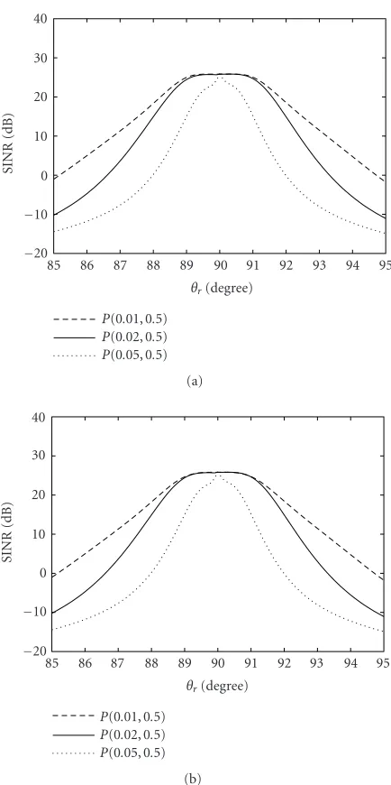
Figure3: SINR for various values ofε. (a) True solution. (b) Ap-proximated solution.
respectively. The signal-to-interference-plus-noise ratio (SINR) is then defined by
SINR= Pd Pi+Pe.
(35)
Let the actual and prescribed DOAs of the desired signal be θrandθd, respectively. We putθd = 90◦to design the con-straint vectorc, and computed the weight vectorwfor vari-ous values ofθr.Figure 2plots the SINR as the function ofθr. The result for the conventional array computed by (3) is also shown for comparison purposes. It is found that the robust array offers a flat SINR in the look direction, although there is a tradeoffin the noise rejection capability of the processor in look directions which are far away from the desired signal.
Figure 3shows the SINRs for ε = 0.01, 0.02, and 0.05
40 30 20 10 0
−10
−20
SINR
(dB)
85 86 87 88 89 90 91 92 93 94 95 θr(degree)
P(0.02, 0.3) P(0.02, 0.5) P(0.02, 1)
(a)
40 30 20 10 0
−10
−20
SINR
(dB)
85 86 87 88 89 90 91 92 93 94 95 θr(degree)
P(0.02, 0.3) P(0.02, 0.5) P(0.02, 1)
(b)
Figure4: SINR for various values of∆. (a) True solution. (b) Ap-proximated solution.
exact and approximated solutions, respectively, andP(a,b) denotes the result forε =aand∆= b. The exact solution was obtained by (11) and (12), and the approximated solu-tion was obtained by (18) and (30). We see that robustness against look-direction errors is increased asεis smaller, while resolution capability of the desired and interference signals is decreased. Therefore, we have to make a tradeoffbetween ro-bustness and resolution capability in determining the value ofε. We also see that the exact and approximated solutions are very close to each other.
Figure 4shows the SINRs for ∆ = 0.3◦, 0.5◦, and 1.0◦
withε=0.02. We see that robustness against look-direction
40 30 20 10 0
−10
−20
SINR
(dB)
85 86 87 88 89 90 91 92 93 94 95 θr(degree)
Q(0.01) Q(0.1) Q(1)
(a)
40 30 20 10 0
−10
−20
SINR
(dB)
85 86 87 88 89 90 91 92 93 94 95 θr(degree)
Q(0.01) Q(0.1) Q(1)
(b)
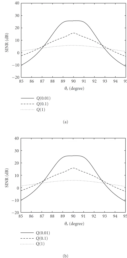
Figure5: SINR for various values of SNR. (a) True solution. (b) Approximated solution.
errors is increased as∆is larger, while resolution capability is decreased.Figure 5shows the SINRs forσ2
n =0.01, 0.1, and 1 withε=0.02 and∆=0.5◦, whereQ(c) denotes the result forσ2
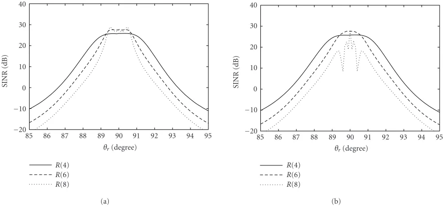
n=c.Figure 6shows the SINRs forN=4, 6, and 8 with
ε=0.02,∆=0.5◦,σ2
n=0.01, whereR(d) denotes the result forN=d. We see that robustness is decreased asσ2
nis larger orN is larger. We also see that the exact and approximated solutions are very close to each other except for the case of N=8.
40 30 20 10 0
−10
−20
SINR
(dB)
85 86 87 88 89 90 91 92 93 94 95 θr(degree)
R(4) R(6) R(8)
(a)
40 30 20 10 0
−10
−20
SINR
(dB)
85 86 87 88 89 90 91 92 93 94 95 θr(degree)
R(4) R(6) R(8)
(b)
Figure6: SINR for various numbers of array elements. (a) True solution. (b) Approximated solution.
Table1: Approximation accuracies.
N σ2
n ε ∆ λ λ |w−w|2 |w−w|2/|w|2 4 0.01 0.02 0.5 24.6107 24.5686 7.44582e-08 2.97194e-07 4 0.01 0.01 0.5 49.963 49.6534 3.14965e-07 1.23124e-06 4 0.01 0.03 0.5 16.2252 16.2136 3.14146e-08 1.28040e-07 4 0.01 0.05 0.5 9.52998 9.52965 1.02032e-08 4.33819e-08 4 0.01 0.02 0.3 24.5805 24.5686 1.33783e-09 5.35673e-09 4 0.01 0.02 1 24.7523 24.5986 1.51836e-05 5.86991e-05 4 0.1 0.02 0.5 25.1836 25.1605 9.75074e-10 3.91061e-09 4 1 0.02 0.5 30.9070 30.9052 1.31363e-11 5.27997e-11 6 0.01 0.02 0.5 24.5654 24.5569 3.25641e-06 1.92091e-05 8 0.01 0.02 0.5 24.5626 24.5561 2.76087e-05 0.000189067
approximated Lagrange multipliers, the squared error be-tween the true and approximated weights, and the normal-ized error. The approximation is found to be very accurate.
Figure 7plots the normalized error between the true and
ap-proximated weights as the function of the angle width ∆, whereFigure 7ais the result forε=0.01, 0.02, 0.05,Figure 7b
is the result forσ2
n=0.01, 0.1, 1, andFigure 7cis the result for N =4, 6, 8. It is evident that the normalized error increases with an increase of∆.
Finally, we compared the robust array trained by the pro-posed algorithm to the conventional array trained by the SMI algorithm in convergence performance.Figure 8depicts the convergence trajectories of the SINR, where Figures8aand
8bare the results for θr = 90◦ andθr = 91◦, respectively. We used the same parameters as in Figure 2. We see from
Figure 8athat both methods show almost the same
perfor-mance in the absence of look-direction errors. We see from
Figure 8b that the conventional method fails when there is
a mismatch between the prescribed and actual DOAs, while the proposed method exhibits almost the same convergence performance due to its robustness against look-direction er-rors.
5. CONCLUSION
We have derived the adaptive weight computation algorithm for the robust array antenna based on the SMI technique by using second-order Taylor series approximations. The adap-tive algorithm can recursively compute the weight vector in only O(N2) computation time. Simulation results have
102 100 10−2 10−4 10−6 10−8 10−10 10−12 10−14 10−16
No
rm
al
iz
ed
er
ro
r
(l
o
g)
0 0.5 1 1.5
∆(degree) ε=0.01
ε=0.02 ε=0.05
(a) 102
100 10−2 10−4 10−6 10−8 10−10 10−12 10−14 10−16
No
rm
al
iz
ed
er
ro
r
(l
o
g)
0 0.5 1 1.5
∆(degree) σ2
n=0.01 σ2
n=0.1 σ2
n=1 (b) 102
100 10−2 10−4 10−6 10−8 10−10 10−12 10−14 10−16
No
rm
al
iz
ed
er
ro
r
(l
o
g)
0 0.5 1 1.5
∆(degree) N=4
N=6 N=8
(c)
Figure 7: Approximation accuracies: (a) Case I (ε =
0.01, 0.02, 0.05). (b) Case II (σ2
n = 0.01, 0.1, 1). (c) Case III (N=4, 6, 8).
30
20
10
0
−10
SINR
(dB)
0 1000 2000 3000
Sample Conventional Proposed
(a) 30
20
10
0
−10
SINR
(dB)
0 1000 2000 3000
Sample Conventional Proposed
(b)
Figure8: Convergence comparisons. (a)θr=90◦. (b)θr=91◦.
The inequality constraint for the case of broadband sources was considered in [14,16]. Using the same approx-imation method, the result for a narrowband source will be extended to broadband sources.
REFERENCES
[1] O. L. Frost III, “An algorithm for linearly constrained adaptive array processing,” Proceedings of the IEEE, vol. 60, no. 8, pp. 926–935, 1972.
[2] K. Takao, M. Fujita, and T. Nishi, “An adaptive antenna ar-ray under directional constraint,” IEEE Trans. Antennas and Propagation, vol. 24, no. 5, pp. 662–669, 1976.
[3] H. Cox, “Resolving powers and sensitivity to mismatch of optimum array processors,”Journal of the Acoustical Society of America, vol. 54, no. 3, pp. 771–785, 1973.
[5] M. H. Er and A. Cantoni, “Derivative constraints for broad-band element space antenna array processors,” IEEE Trans. Acoustics, Speech, and Signal Processing, vol. 31, no. 6, pp. 1378–1393, 1983.
[6] K. M. Buckley and L. J. Griffiths, “An adaptive general-ized sidelobe canceller with derivative constraints,” IEEE Trans. Antennas and Propagation, vol. 34, no. 3, pp. 311–319, 1986.
[7] H. Cox, R. M. Zeskind, and M. M. Owen, “Robust adaptive beamforming,”IEEE Trans. Acoustics, Speech, and Signal Pro-cessing, vol. 35, no. 10, pp. 1365–1376, 1987.
[8] C.-Y. Tseng, “Minimum variance beamforming with phase-independent derivative constraints,” IEEE Trans. Antennas and Propagation, vol. 40, no. 3, pp. 285–294, 1992.
[9] I. Thng, A. Cantoni, and Y. H. Leung, “Derivative constrained optimum broad-band antenna arrays,” IEEE Trans. Signal Processing, vol. 41, no. 7, pp. 2376–2388, 1993.
[10] R. J. Evans and K. M. Ahmed, “Robust adaptive array anten-nas,” Journal of the Acoustical Society of America, vol. 71, no. 2, pp. 384–394, 1982.
[11] K. M. Ahmed and R. J. Evans, “An adaptive array pro-cessor with robustness and broad-band capabilities,” IEEE Trans. Antennas and Propagation, vol. 32, no. 9, pp. 944–950, 1984.
[12] K. Takao and N. Kikuma, “Tamed adaptive antenna array,” IEEE Trans. Antennas and Propagation, vol. 34, no. 3, pp. 388– 394, 1986.
[13] A. Cantoni, X. G. Lin, and K. L. Teo, “A new approach to the optimization of robust antenna array processors,”IEEE Trans. Antennas and Propagation, vol. 41, no. 4, pp. 403–411, 1993. [14] M. H. Er and A. Cantoni, “A new approach to the design of
broad-band element space antenna array processors,” IEEE Journal of Oceanic Engineering, vol. 10, no. 3, pp. 231–240, 1985.
[15] M. H. Er and A. Cantoni, “A new set of linear constraints for broad-band time domain element space processors,”IEEE Trans. Antennas and Propagation, vol. 34, no. 3, pp. 320–329, 1986.
[16] M. H. Er and A. Cantoni, “A unified approach to the design of robust narrow-band antenna array processors,”IEEE Trans. Antennas and Propagation, vol. 38, no. 1, pp. 17–23, 1990. [17] I. S. Reed, J. D. Mallett, and L. E. Brennan, “Rapid
conver-gence rate in adaptive arrays,”IEEE Transactions on Aerospace and Electronic Systems, vol. 10, no. 6, pp. 853–863, 1974. [18] K. Gerlach and F. F. Kretschmer Jr., “Convergence properties
of Gram-Schmidt and SMI adaptive algorithms,”IEEE Trans-actions on Aerospace and Electronic Systems, vol. 26, no. 1, pp. 44–56, 1990.
[19] G. H. Golub and C. F. Van Loan,Matrix Computations, Johns Hopkins University Press, Baltimore, Md, USA, 3rd edition, 1996.
[20] W. Gander, “Least squares with a quadratic constraint,” Nu-merische Mathematik, vol. 36, no. 3, pp. 291–307, 1981.
Tomoaki Yoshida received the B.E. and M.E. degrees in the communications en-gineering from Osaka University, Osaka, Japan, in 1996 and 1998, respectively. In 1998, he joined NTT Access Network Ser-vice Systems Laboratories, Chiba, Japan. He has been engaged in research on next-generation optical access network and sys-tems.