R E S E A R C H
Open Access
SAR target recognition based on improved joint
sparse representation
Jian Cheng
*, Lan Li, Hongsheng Li and Feng Wang
Abstract
In this paper, a SAR target recognition method is proposed based on the improved joint sparse representation (IJSR) model. The IJSR model can effectively combine multiple-view SAR images from the same physical target to improve the recognition performance. The classification process contains two stages. Convex relaxation is used to obtain support sample candidates with theℓ1-norm minimization in the first stage. The low-rank matrix recovery strategy is introduced to explore the final support samples and its corresponding sparse representation coefficient matrix in the second stage. Finally, with the minimal reconstruction residual strategy, we can make the SAR target classification. The experimental results on the MSTAR database show the recognition performance outperforms state-of-the-art methods, such as the joint sparse representation classification (JSRC) method and the sparse representation classification (SRC) method.
Keywords:SAR target recognition; Sparse representation; Low-rank matrix recovery; Multiple views
1 Introduction
Synthetic aperture radar (SAR) is a high-resolution imaging radar. It can work regardless of climatic circumstances and time constraint. Thus, it is widely applied in kinds of mili-tary and civilian areas such as disaster assessment, resource exploration, and battlefield reconnaissance. SAR target rec-ognition plays an important role in the automatic analysis and interpretation of the SAR image data. Over the past several decades, although lots of algorithms are exploited in SAR target recognition [1-3], it is a challenging issue due to the complexity of the measured information such as speckle noises, variation of azimuth, and poor visibility. Therefore, there is still no commonly agreed-upon system that settles SAR target recognition so far.
SAR target recognition includes two important parts, feature extraction and classifier construction. For feature extraction, classic methods, such as principal component analysis (PCA) [4], independent component analysis (ICA) [5], linear discriminant analysis (LDA) [6], nonnegative matrix factorization (NMF) [7,8], and their improved algo-rithms [9], have been successfully used in SAR target recognition. Beyond those, in consideration of most fea-tures in nature distributing as a manifold structure, the
manifold-based feature extraction algorithms become a new trend [10,11]. Though kinds of feature extraction methods have their own advantages, no method exten-sively can be accepted. As for the classifier, support vector
machine (SVM) and K-nearest neighbor (KNN) are the
most common choices. To improve the performance of SAR target recognition, the classifying results under differ-ent features are fused to make the final classifier [12]. In addition, sparse representation which closely bonds the feature extraction with the classifier has gradually aroused researchers' attention. Some advantages of sparse repre-sentation for recognition are mentioned in [13] such as its insensitivity to feature extraction method under certain conditions and the natural discriminative information in sparse representation coefficients, i.e., feature extraction is implicit in recognition and the classifier can be designed according to the sparse representation coefficients. The re-sults for face recognition show the great competitiveness compared with other methods [13]. Due to these advan-tages of sparse representation, Thiagarajan et al. [14] and Estabridis [15] both introduced sparse representation in target recognition. Thiagarajan et al. explained sparse rep-resentation from the point of manifold, which indicates the strength of sparse representation for SAR target recog-nition. They selected random projections as the feature extraction method and solved sparse representation using * Correspondence:[email protected]
School of Electronic Engineering, University of Electronic Science and Technology of China, 611731 Chengdu, Sichuan, People's Republic of China
the greedy algorithm. Knee et al. [16] used image parti-tioning and sparse representation based feature to handle SAR target recognition.
The preceding methods only take one SAR image as the input signal to decide which class the target in the image belongs to. In practice, we can obtain multiple-view SAR images of the same physical target. Thus, some tried to make use of multiple-view SAR images under the the-ory framework of sparse representation. Exploring the sparse representation for the multiple input signals at the same time is a joint sparse representation problem [17,18]. Therefore, Zhang et al. [19] used the joint sparse represen-tation (JSR) model to seek common sparse patterns between multiple-view SAR images. In the JSR model, multiple-view SAR images are integrated in a matrix form. Under this context, the JSR model finally becomes a mixed-norm problem. An efficient and accurate greedy al-gorithm, CoSaMP [20,21], is utilized to solve the model, and the classification algorithm is named as joint sparse representation classification (JSRC) which is similar with sparse representation classification (SRC).
With the inspiration from the JSR model, we propose an improved joint sparse representation (IJSR) model for SAR target recognition with multiple-view images. Com-pared with the original JSR model, there are two im-provements in the IJSR model. The first is that sparse representation for the single-view image is described by
aℓ1-norm minimization model. The second is that
com-mon patterns in sparse representation coefficients of multiple-view images are sought by low-rank matrix
re-covery. Theℓ1-norm minimization model has two
bene-fits for SAR target recognition. One benefit is that the proper sparse level parameter which is hard to choose in the original JSR model is not needed anymore. Another benefit is that sparse representation coefficients of theℓ1
-norm minimization are more concentrated in one class, which enhances the discrimination of sparse representa-tion coefficients. Different from the greedy algorithm in the original JSR model, theℓ1-norm minimization usually
produces more nonzero entries in sparse representation coefficients of SAR target images. With the excessive non-zero entries, it becomes difficult to seek support samples which refer to the samples in the dictionary that associate with the nonzero entries in sparse representation coeffi-cients. To tackle this problem, we further make some hy-potheses that the matrix of joint sparse representation coefficients associating with support samples is low rank, and the rest that excludes the joint sparse representation coefficients associating with support samples is a sparse matrix. These hypotheses are based on the following rea-sons. According to the common sparse pattern assump-tion in the JSR model, these images with close views share the same support sample set. The common sparse pattern means important sparse representation coefficients which
correspond to the support sample set have the same in-dexes in the dictionary and occupy the most nonzero en-tries in sparse representation coefficients. The problem of seeking the support samples converts to a low-rank matrix recovery problem; meanwhile, the low-rank matrix recov-ery algorithm could directly obtain the proper sparse rep-resentation coefficients on support samples.
The paper is organized as follows: In Section 2, we re-view the joint sparse representation model and describe the classification strategy. Section 3 analyzes the disad-vantages of joint sparse representation and proposes the improved joint sparse representation model along with the classification strategy. In Section 4, we verify the proposed method with experiments on publicly available MSTAR database and compare with the classical SRC method and the original JSRC method.
2 Joint sparse representation for SAR target recognition
In the real scenario, the multiple-view SAR images from one same target can be captured, and those images are highly correlated. When a uniform dictionary is used for these multiple-view images' sparse representation, an im-plicit correlation in the sparse representation coefficients can emerge. The correlation is defined as the common pat-terns which specifically mean the same positions of the nonzero entries in the sparse representation coefficients in the work of Zhang et al. [19]. The JSR model, which can combine the sparse representation coefficients of multiple-view images to extract the common patterns, is introduced in SAR target recognition.
2.1 Joint sparse representation model
Supposing each image under different views has been translated to a vectoryj, given Jviews of the same phys-ical target, the J sparse representation problems can be defined together as
where D is the dictionary which usually consists of the
training sample vectors, xj is the sparse representation
coefficient vector associating with the jth inputting image
vector yj, and K is a preset parameter that controls the
sparse level. Using the matrix notationsX¼½x1;x2;…;xJ,
where‖·‖ℱrepresents the Frobenius norm which
and ‖·‖0is the ℓ0-norm of the matrix, which is defined
as the number of nonzero entries in the matrix. Since X^
is decomposed to compute the column one by one, this model cannot embody the correlation information be-tween the multiple-view SAR images. To combine the sparse representation coefficients under the multiple views, an assumption that the multiple views of the same physical target share a common pattern in their sparse representation coefficient vector with respect to the same dictionary is made. The common pattern means the indexes of atoms in the dictionary that participate in the linear reconstruction of the inputting SAR images are the same for multiple-view SAR images, though the coefficients corresponding to the same atom may be dif-ferent for each view. Specifically, this assumption allows
all theJobservations sparsely represented by a same small
set of atoms selected from the dictionary while weighted with different coefficient values. This can be achieved by
solving an optimization problem with the ℓ0/ℓ2
mixed-norm regularization as
which is defined by two computing processes. Firstly,
the ℓ2-norm is applied on each row of the matrix, and
then theℓ0-norm of the resulting vector is computed as
the result of the mixed-norm. The K training samples
corresponding to the nonzero entries in the resulting vector are the support samples whose class labels reflect the label of the testing SAR target in some sense. The number of support samples is usually far less than the total number of samples.
2.2 Joint sparse representation classification
The classification strategy for the JSR model is similar with the SRC model, and the minimal reconstruction re-sidual/error criterion is used. The classification model is defined as
with only the cth training samples involve in the
recon-struction, and the operationδc(∙) is redefined as preserving
the rows corresponding to classcin the matrixXand
set-ting all others to be zeroes. The Frobenius norm indicates that the decision is based on the total reconstruction error of multiple views. This whole classification algorithm is named as JSRC, and greedy algorithm can solve this problem in an approximate sense. Since greedy algorithm is one way to solve sparse representation without any
transformation for the original sparse representation model,
we call itℓ0-norm model/minimization in this paper.
3 Improved joint sparse representation
In the JSR model, the common pattern is sought on the
ℓ0-norm minimization model whose performance
de-pends on a proper choice of parameterK. According to
the ℓ0-norm minimization, the mixed-norm strategy is
used to explore the common patterns in sparse repre-sentation coefficients of multiple SAR images. However, the properKis hard to determine. Therefore, in this sec-tion, we propose an improved joint sparse representation model which firstly replaces ℓ0-norm minimization with
ℓ1-norm minimization to avoid the parameterKselection
problem and then adopts the low-rank matrix recovery strategy to seek the common patterns based on the char-acteristics of theℓ1-norm minimization solutions.
3.1 Improved joint sparse representation model
As Section 2.2 says, greedy algorithm is one way to solve sparse representation in the approximate sense. Another way, which has strong theoretical foundations, is convex relaxation. Under the theoretical framework of convex relaxation, theℓ0-norm in the original sparse
representa-tion model is replaced with the ℓ1-norm, and then the
original model is converted as a convex quadratic pro-gramming problem. This solving strategy is called theℓ1
-norm minimization in this paper. Zhang et al. did not dis-cuss the possibility to use convex relaxation in the JSR model [19]. So, we firstly explore the potentiality of theℓ1
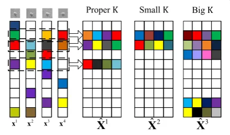
-norm minimization through an elaborate experiment. There is a key parameterKin the JSR model. It represents the sparse level of the inputting signals and needs to be set manually. However, no algorithm can predictKaccurately, andKmay be a variable even with a fixed number of views. Figure 1 gives a pictorial illustration for the JSR coefficient matrix with different parameter K. Dimensionality of each
1
Figure 1The JSR coefficient matrix with different parameterK.The sparse representation coefficients from four views denoted as xj 4j¼1
and the JSR coefficients matrix denoted asn oX^i 3
sparse representation coefficient vector is 10, and every entry in sparse representation coefficient vector is repre-sented with one block. Colored blocks indicate nonzero en-tries and white blocks indicate zero enen-tries. Let us assume that the first five blocks in each sparse representation vector correspond to the samples from one same class, and the rest correspond to the sample set of another class. To demon-strate the performance of the different parameterK, we sup-pose the SAR images are from the first class target in Figure 1. If a proper parameterKis set, all support samples in the JSR coefficient matrix will concentrate in the first class which is shown asX^1. However, the perfect choice of the parameter Kis very difficult in real situation. If a too smallKis selected, a JSR coefficient matrix with less support samples would be obtained.X^2is the JSR coefficient matrix withK= 2. Though support samples inX^2 are still from the first class, the reconstruction error becomes bigger with less support samples. In worse case, if SAR images from differ-ent classes are similar, the support samples will distribute on different classes. Under this context, the recognition be-comes more difficult. If a too bigKis chosen, the JSR coeffi-cient matrix would contain more support samples as X^3
whose parameter K is 5. As Figure 1 shows, the support
samples scatter on different classes, and it results in two close residuals that may classify the target to the second
class. To avoid seeking the perfectK,ℓ0-norm minimization
is replaced withℓ1-norm minimization without setting the
parameterK.
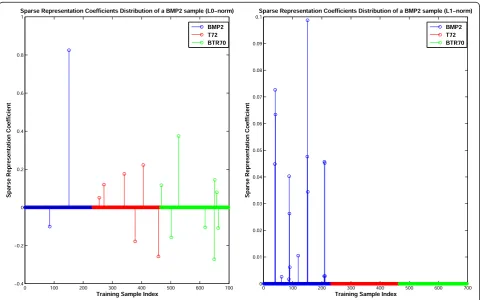
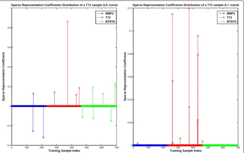
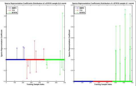
A more important motivation behind this replacement is that a more discriminative ability is shown with the ℓ1-norm minimization in SAR target recognition
accord-ing to our experiments. In our experiments, two kinds of sparse representation coefficients of three samples from BMP2, T72, and BTR70, which are the class labels in the public database MSTAR, are shown in Figures 2, 3, and 4. One kind of sparse representation coefficients is obtained viaℓ0-norm minimization and another one is
solved through ℓ1-norm minimization. To be fair, we
firstly solve ℓ1-norm minimization, and then, according
to the number of nonzero entries in the ℓ1-norm
solu-tion, we specify the number of nonzero entries which is defined as the parameterKin theℓ0-norm solution. The
dictionary is composed of 698 training samples. Each dictionary atom index in Figures 2, 3, and 4 is associated with one training sample. The first 233 training samples are from BMP2. The coefficients associated with BMP2 are presented in blue lines which are ended up with a blue circle mark. The training samples that have index from 234 to 465 belong to T72, and the corresponding coefficients are indicated as red lines with a red circle
mark in their ends. The rest of the training samples, whose coefficients are described by green lines with the green circle mark in their tails, come from BTR70. Though some big coefficients exist in theℓ0-norm
solu-tion, sparse representation coefficients scatter on differ-ent classes. Meanwhile, the coefficidiffer-ents of the ℓ1-norm
solution almost concentrate on one class as well as the right class. Obviously, more concentrated coefficients re-veal more discriminative information.
With the experimental results and the analysis, we adopt theℓ1-norm minimization based algorithm to solve sparse
representation coefficients for SAR image under each view. Theℓ1-norm minimization model can be expressed as
^
xj Jj¼1¼ min
^
xj
f gJ j¼1
XJ
j¼1
xj 1
subject to yj−Dxj
ℱ≤;∀1≤j≤J;
ð5Þ
This model can be solved by computing the sparse representation coefficient vectors one by one as well. However, there are another two problems for theℓ1-norm
minimization model. First, the solution x^j Jj¼1 using (5)
usually contains more nonzero items. In ideal case, we ex-pect a few nonzero items in ^xj Jj¼1 because this can give us
a clear position indication of support samples. Second, the sparse representation coefficients of each inputting image with close azimuth are obtained independently. Therefore, the combination between multiple-view im-ages is lacking, which makes the solution lost the joint-ing meanjoint-ing.
Although the sparse representation coefficients from different views may be different in the coefficient distri-bution, they share most support samples. The sparse representation coefficients ^xj; j¼1;…;J with J views can be combined as the matrixX^ ¼½^x1; ^x2;…;x^J. Non-zero items associated with support samples in sparse rep-resentation coefficients occupy the majority. With this characteristics, we can consider that the matrixX^ is com-posed of a joint sparse representation coefficient matrixS that is named as the signal matrix and a noise matrixN.
Since the number of nonzero entries ofS is expected to
into a low-rank matrix recovery problem. The low-rank matrix recovery can be defined as
min
S;N rankð Þ þS λk kN 0 subject to X^¼SþN ð6Þ
where rank(∙) stands for the rank of matrix and λ
bal-ances the rank of the signal matrixSand theℓ0-norm of
the noise matrix N. Since it is hard to find the solution
of (6), some relaxations are made to simplify it. The
op-eration rank(∙) is replaced with the nuclear norm ‖·‖*
which computes the sum of singular values of a matrix,
and the operation ‖·‖0 is substituted with operation
‖·‖1which is defined by adding every absolute value of
entries in the matrix. Then, (6) can be rewritten as (7). This becomes a robust principal component analysis problem [22].
min
S;N k kS þλk kN 1 subject to X¼SþN ð7Þ
Apparently, the rank of the signal matrix rank(S) in
the JSR matrix, the number of view J, and the proper
sparse levelKhave close relations, which affects the rec-ognition performance in some sense. With consideration of the computation cost, the number of views should be limited in a proper range. Generally,Jis far less than the dimensionality of the inputting sparse representation
coefficient vector. Therefore, the maximal rank of the signal matrix is definitely no more than the number of views. When rank(S) <K, the nonzero entries with the same indexes are not enough to reveal real support sam-ples. The support samples in this case tend to be the
lin-ear combinations of Kreal support samples, which also
can make the right recognition. When rank(S) =K, the low-rank matrixSis very likely to attain theKreal sup-port samples which contains explicit classification infor-mation. This is the best situation for recognition. When rank(S) >K, the low-rank matrixSfails to find the support samples. As a result, small coefficients tend to appear on nonsupport sample to meet the low-rank condition, while most sparse representation coefficients solved by (5) will remain in the signal matrix S. The reconstruction to the multiple-view SAR images may become worse than the re-construction by ℓ1-norm solutions in (5) as small
coeffi-cients' influence. However, the recognition is still right for most cases due to the sparse representation coefficients via (5) almost concentrating on one class.
According to the above analysis, the IJSR model can be described as two stages. The first stage is seeking the ℓ1-norm solutions for multiple-view SAR images via (5).
The second stage is combining the ℓ1-norm solutions
from the JSR model, in the first stage, the ℓ1-norm
minimization in the IJSR model avoids choosing a proper sparse level which is hard to predict. In addition,
the solution for the ℓ1-norm minimization contains
more discriminative information. In the second stage, discarding the mixed-norm strategy in JSR, the problem of finding the support samples is converted into a low-rank matrix recovery problem.
3.2 Improved joint sparse representation classification
Similar with the classification strategy in SRC and JSRC, we classify a testing sample based on how well the new low-rank matrix associated with each class re-produces the testing sample under J views. δcðÞ is an
operator that has the same meaning with δcðÞin
Sec-tion 2.2. Here, δcð ÞS represents a new matrix whose
nonzero entries are the entries in the matrixS
associ-ated with classc. Let S¼ ST
1;…;STc;…;STC
T
, Cis the
number of class, and the sub-matrix Sc stands for a
matrix composed of rows in Sassociated with the cth
class. Then, δcð ÞS can be defined as δcð Þ ¼S
0T1;…;0Tc−1;STc;0Tcþ1;…;0TC
T
. The given testing sample
matrix underJviews can be approximated as
Yc¼Dδcð ÞS ð8Þ
Based on the approximation residuals on each class, we can make the classification by the minimum approxi-mation residual criteria, which can be described as
^c¼ min
c kY−Yckℱ ð9Þ
The improved JSR classification (IJSRC) algorithm is summarized in Algorithm 1.
4 Experiments
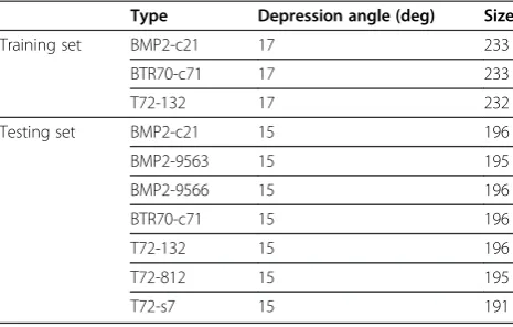
In this section, our experiments are implemented on the public database MSTAR. All SAR images in the MSTAR database are X-band with 0.3 m × 0.3 m resolution.
Three kinds of targets with depression angle 17° are
chosen as the training samples and seven categories with depression angle 15° as the testing samples. The depres-sion angle, class, serial number, and sample size are listed in Table 1.
The database is firstly preprocessed as follows: The logarithm transformation is made to turn the multiplica-tive speckle to the addimultiplica-tive noise. To reduce the disturb-ance from the background of SAR image, a 50 × 50 sub-image which mainly contains the SAR target is ex-tracted in the center of the original SAR image. Then, PCA is used as the feature extraction algorithm for its convenience and effectiveness.
4.1 One important precondition
azimuths. Another group of images has close azimuths. The dictionary atoms belong to BMP2-c21 with depres-sion angle 17°. There are 233 training samples (i.e., 233 dictionary atoms). For convenience, we use the greedy algorithm to select the support samples. The number of support samples is set as 5 in this experiment. The test-ing sample and correspondtest-ing support samples indexes are shown in Tables 2 to 3.
The testing samples have greatly different azimuths in Table 2 and have close azimuths in Table 3. As shown in Table 3, five samples with close azimuths apparently have a more similar support sample set. For the samples with greatly different azimuths, the common support samples cannot be found as example in Table 2. It is ob-vious that the right recognition cannot be made if we adopt testing samples in Table 2. Therefore, we expect more samples with a closer azimuth interval in practice. Fortunately, in real case, one can capture more SAR im-ages of one physical target in a much smaller azimuth interval. In this paper, all experiments are performed under the condition that multiple-view images have close azimuths.
4.2 Experimental results and discussions
To demonstrate the performance, our proposed IJSRC al-gorithm is compared with the state-of-the-art methods,
such as SRC [13] and JSRC [19]. Since the SRC algorithm is applied for the single image, the comparison experiment is implemented by concatenating the images underJviews as a vector to form the final inputting vector in SRC. Then, the multiple-view sparse representation could be regarded as a single-view problem and solved by SRC. The SLEP toolkit [23] is applied for seeking theℓ1-norm
solu-tions in IJSRC. Considering the efficiency as well as the ac-curacy, we still use CoSaMP greedy algorithm in JSRC as [19] does.
The first experiment is implemented to show the rec-ognition performance of SRC, JSRC, and IJSRC with dif-ferent feature dimensionalities. The results are shown in Figure 5. IJSRC outperforms SRC and JSRC when the dimension is less than 160. IJSRC achieves maximum recognition rate 98.535% with dimension 48. The max-imum recognition rates for JSRC and SRC are 98.022% and 97.363%. That is to say, IJSRC performs better in low dimension. This result can well fit the practical re-quirement that SAR target recognition systems hope a better recognition result with a lower feature dimension. However, the recognition rate of IJSRC decreases with increasing of dimension, especially when the dimension exceeds 160. There is one reason in our opinion. Since the noises exist both in training samples and testing samples, the noises become strong with the increasing of the feature dimensionality, which can reduce the rele-vance of features for the multiple-view SAR images. Therefore, an improper low-rank matrix is generated by IJSRC, which leads to a bad recognition.
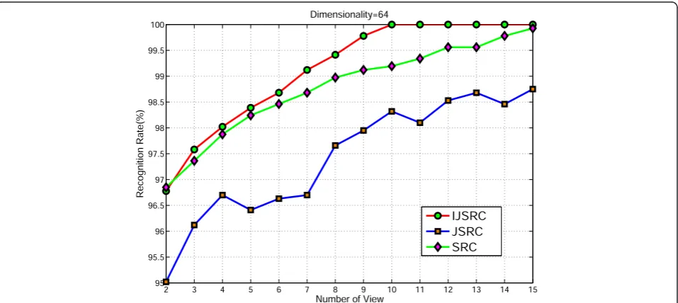
In the second experiment, we compare the recognition performance of SRC, JSRC, and IJSRC with different number of views. Figure 6 shows the recognition results with the dimensionality fixed as 64. Three approaches all present the ascending trend along with the increase of the number of view. Recognition rate of IJSRC grows faster than one of JSRC and SRC. As for the best recog-nition performance, the maximal recogrecog-nition rate of JSRC is 98.75% and the maximal recognition rate for SRC is 99.927%, both with the number of view as high as 15. In comparison, IJSRC reaches 100% when the number of view reachesJ≥10.
Table 2 The support sample indexes of five samples with greatly different azimuths
3 243.0678 28, 171, 198, 199, 200
4 301.0678 38, 40, 87, 88, 150
5 336.0678 44, 96, 158, 159, 160
Table 3 The support sample indexes of five samples with close azimuths
Testing sample number
Azimuth (deg) Support sample set indexes
1 243.0678 28, 171, 198, 199, 200
2 244.0678 27, 28, 139, 198, 199
3 248.0678 29, 140, 142, 199, 200
4 249.0678 29, 30, 140, 199, 201
5 250.0678 30, 140, 199, 200, 201
Table 1 Experimental database information
Type Depression angle (deg) Size
Training set BMP2-c21 17 233
BTR70-c71 17 233
T72-132 17 232
Testing set BMP2-c21 15 196
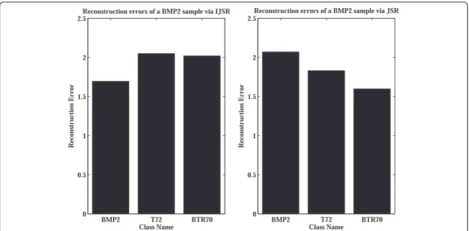
Since IJSRC is improved on the foundation of JSRC, the third experiment is carried to exhibit the improve-ment of IJSRC through reconstructing the feature matrix of testing samples. Figures 7, 8 and 9 give the recon-struction errors of three examples from three classes by using the IJSR model and the JSR model, respectively. Three black bars in each subplot denote the reconstruc-tion errors on three classes. As the reconstrucreconstruc-tion errors shown in Figure 7, JSRC gives a wrong prediction while IJSRC makes a right decision according to the minimum approximation residual criteria. For the class BMP2, the
reconstruction error using the JSR model is maximal, which is the worst case in recognition. Figure 8 shows the situation that the JSR model infers a wrong result while the IJSR model obtains the right predication of the class label with a slightly smaller reconstruction error on T72 than on BMP2. In Figure 9, both the JSR model and the IJSR model can make the right prediction. However, the IJSR model slightly outperforms the JSR model with a smaller reconstruction error. Actually, the recognition rate of both the JSR model and the IJSR model can reach 100% on the class BTR70. Though we sometimes find Figure 5Recognition rates of SRC, JSRC, and IJSRC.The number of view is fixed as 5 and the dimensionality ranges from 32 to 320.
that the reconstruction error on the right class in the JSR model is slightly smaller than the reconstruction error on the right class in the IJSR model, this situation tends to happen when the reconstruction errors on the right class are both remarkably smaller than the
reconstruction errors on the wrong class. That is to say, though the IJSRC algorithm may have poor reconstruc-tion to the inputting SAR images, the right recognireconstruc-tion result is still guaranteed. This phenomenon fits the ana-lysis with regard to rank(S) >Kin Section 3.2. In most Figure 7Reconstruction errors of a BMP2 sample via IJSR model and JSR model, respectively.
cases, the reconstruction via IJSRC outperforms the re-construction with JSRC according to our experiment. Therefore, the IJSR model outperforms the JSR model generally.
5 Conclusions
An IJSR model for SAR target recognition under mul-tiple views is proposed in this paper. In the IJSR model,
the ℓ0-norm minimization is replaced by the ℓ1-norm
minimization to solve the sparse representation of single-view SAR image, which can overcome the problem of choosing the proper sparse level and concentrates sparse representation coefficients in one class. Moreover, the low-rank matrix recovery strategy is proposed to seek the common support samples for SAR target recognition under multiple views. Experiments on the MSTAR data-base show that our algorithm outperforms JSRC and SRC in a low-dimensional feature space. With the increase of the number of view, the recognition rates of IJSRC in-crease faster and reach a higher point than those of JSRC and SRC. In conclusion, IJSRC generally outperforms JSRC and SRC.
Competing interests
The authors declare that they have no competing interests.
Acknowledgements
This research was supported by the National Natural Science Foundation of China (61201271, 61301269), the Fundamental Research Funds for the
Central Universities (ZYGX2013J019, ZYGX2013J017), and the Sichuan Science and Technology Support Program (cooperated with the Chinese Academy of Sciences) (2012JZ001).
Received: 26 February 2014 Accepted: 16 May 2014 Published: 9 June 2014
References
1. Q Zhao, JC Principe, Support vector machines for SAR automatic target recognition. IEEE Trans. Aerosp. Electron. Syst.37(2), 643–654 (2001) 2. C Nilubol, RM Mersereau, MJ Smith, A SAR target classifier using radon
transforms and hidden Markov models. Digital Sig. Proce. 12(2), 274–283 (2002)
3. Y Sun, ZP Liu, S Todorovic, J Li, Adaptive boosting for SAR automatic target recognition. IEEE Trans. Aerosp. Electron. Syst.43(1), 112–125 (2007) 4. Z He, J Lu, G Kuang, A fast SAR target recognition approach using PCA
features, inProceedings of the Fourth International Conference on Image and Graphics(IEEE, Washington, 2007), pp. 580–585
5. Y Yang, Y Qiu, C Lu, Automatic target classification–experiments on the MSTAR SAR images, inProceedings of the Sixth International Conference on Software Engineering, Artificial Intelligence, Networking and Parallel/Distributed Computing, and First ACIS International Workshop on Self-Assembling Wireless Networks(IEEE, Washington, 2005), pp. 2–7
6. AK Mishra, Validation of PCA and LDA for SAR ATR, inProceedings of
TENCON-2008 IEEE Region 10th Conference, 2008(IEEE, Piscataway, 2008),
pp. 1–6
7. R Hong, P Yun, K Mao, SAR image target recognition based on NMF feature extraction and Bayesian decision fusion, inProceedings of IEEE Second IITA International Conference on Geoscience and Remote Sensing (IITA-GRS), 2010, vol. 1 (IEEE, Piscataway, 2010), pp. 496–499
8. Z Cao, J Feng, R Min, Y Pi, NMF and FLD based feature extraction with application to synthetic aperture radar target recognition, inProceedings of
2012 International Conference on Communications(IEEE, Piscataway, 2012),
pp. 6416–6420
and Pacific Conference on Synthetic Aperture Radar(IEEE, Piscataway, 2007), pp. 801–805
10. M Liu, Y Wu, Q Zhao, L Gan, SAR target configuration recognition using locality preserving projections, inProceedings of IEEE CIE International Conference on Radar, vol. 1 (IEEE, Piscataway, 2011), pp. 740–743 11. M Liu, Y Wu, P Zhang, Q Zhang, Y Li, M Li, SAR target configuration
recognition using locality preserving property and Gaussian mixture distribution. IEEE Geosci. Remote Sens. Lett.10(2), 268–272 (2013) 12. Z Cui, Z Cao, J Yang, J Feng, A hierarchical propelled fusion strategy for SAR
automatic target recognition. EURASIP J. Wirel. Commun. Netw. (2013). 10.1186/1687-1499-2013-39
13. J Wright, AY Yang, A Ganesh, SS Sastry, Y Ma, Robust face recognition via sparse representation. IEEE Trans Pattern Anal Mach Intell30(2), 210–227 (2009) 14. JJ Thiagarajan, KN Ramamurthy, P Knee, A Spanias, V Berisha, Sparse
representation for automatic target classification in SAR images, in Proceedings of the 4th International Symposium on Communications, Control and Signal Processing(IEEE, Piscataway, 2010), pp. 1–4
15. K Estabridis, Automatic target recognition via sparse representations, in Proceedings of SPIE 7696, Automatic Target Recognition XX; Acquisition, Tracking, Pointing, and Laser Systems Technologies XXIV; and Optical Pattern Recognition XXI, 76960O, 2010. doi:10.1117/12.849591
16. P Knee, JJ Thiagarajan, KN Ramamurthy, A Spanias, SAR target classification using sparse representations and spatial pyramids, inProceedings of IEEE Radar Conference(IEEE, Piscataway, 2011), pp. 294–298
17. G Obozinski, B Taskar, MI Jordan, Joint covariate selection and joint subspace selection for multiple classification problems. J. Statistics Comput. 20(2), 231–252 (2010)
18. XT Yuan, X Liu, S Yan, Visual classification with multi-task joint sparse representation. IEEE Trans. Image Process.21(10), 4349–4360 (2012) 19. H Zhang, NM Nasrabadi, Y Zhang, TS Huang, Multi-view automatic target
recognition using joint sparse representation. IEEE Trans. Aerosp. Electron. Syst.48(3), 2481–2497 (2012)
20. A Rakotomamonjy, Surveying and comparing simultaneous sparse approximation (or group lasso) algorithms. Signal Process. 91(7), 1505–1526 (2011)
21. MF Duarte, V Cevher, RG Baraniuk, Model-based compressive sensing for signal ensembles, inProceedings of 47th Annual Allerton Conference on
Communication, Control, and Computation(IEEE, Piscataway, 2009),
pp. 244–250
22. EJ Candes, X Li, Y Ma, J Wright, Robust principal component analysis? J. ACM 58(3), 11 (2011). 1–37
23. J Liu, S Ji, J Ye,SLEP: Sparse Learning with Efficient Projections(Arizona State University, 2009). http://www.public.asu.edu/~jye02/Software/SLEP. Accessed 28 Dec 2011
doi:10.1186/1687-6180-2014-87
Cite this article as:Chenget al.:SAR target recognition based on improved joint sparse representation.EURASIP Journal on Advances in Signal Processing20142014:87.
Submit your manuscript to a
journal and benefi t from:
7 Convenient online submission 7 Rigorous peer review
7 Immediate publication on acceptance 7 Open access: articles freely available online 7 High visibility within the fi eld
7 Retaining the copyright to your article