F U L L P A P E R
Open Access
Application of cluster analysis based on
waveform cross-correlation coefficients to data
recorded by ocean-bottom seismometers: results
from off the Kii Peninsula
Takeshi Akuhara
*and Kimihiro Mochizuki
Abstract
Waveform cross-correlation coefficients (CCs) have often been used to investigate clustering of earthquakes. Such techniques, however, have rarely been applied to waveform data recorded by ocean-bottom seismometers (OBSs). The data recorded by some OBSs are strongly influenced by site effects such as the existence of unconsolidated sediment layers. The resulting waveforms tend to have a monotone frequency so that the calculated CCs stay artificially high, and false delay times are obtained at certain multiples of the period. This effect also varies from place to place. To overcome such problems, CC measurements were first performed using multiple time windows with different lengths in order to reject unstable results. Station-specific CC thresholds were then objectively determined based on the CC distributions. This method was applied to seismic measurements obtained by OBSs deployed off the Kii Peninsula from 2003 to 2007 in order to identify characteristic hypocenter patterns. Two types of earthquake clusters were found. The first occurred within the oceanic mantle, and the component events were linearly aligned along the NNE direction. Such earthquakes are considered to occur on preexisting faults due to dehydration of the serpentinized mantle. The second type of cluster consisted of interplate earthquakes that occurred at the southern tip of the Kii Peninsula. These are thought to be the result of stress caused by local structural heterogeneity of the dense rock body.
Keywords:Cross-correlation coefficients; Ocean-bottom seismometers; Subduction zone; Earthquake cluster
Background
Cross-correlation coefficients (CCs) are used to deter-mine the degree of similarity between seismograms. Be-cause an observed seismogram is a convolution of the source term, path effects, site effects, and instrumental responses, earthquake pairs with high CC values are con-sidered to have close hypocenters and similar focal me-chanisms (Baisch et al. 2008). For a variety of reasons, researchers have attempted to link similar earthquakes and group them into clusters. One reason is to detect re-peating earthquakes, which occur at the same asperities on the same fault planes (e.g., Geller and Mueller 1980; Igarashi et al. 2003). Their magnitudes are roughly com-parable, and some of them are characterized by periodic
repetition. Another reason is to determine the spatial pat-terns of hypocenters and associate them with seismogenic structures such as faults (e.g., Cattaneo et al. 1999; Ferretti et al. 2005). In this case, it is not always necessary that similar earthquakes should have comparable magnitudes, and differences in location are also permitted to some ex-tent. A third reason for grouping earthquakes is to more precisely identify their relative locations within clusters by measuring accurate differential travel times based on CC delay times (e.g., Lin and Shearer 2007; Shearer et al. 2005). Such studies require only that the waveforms asso-ciated with the first pulses be similar. Depending on the desired goal, different CC thresholds are introduced to judge the similarity between waveforms.
In spite of these applications, few researchers have ap-plied such cluster analysis techniques to waveform data recorded by ocean-bottom seismometers (OBSs). The
* Correspondence:[email protected]
Earthquake Research Institute, University of Tokyo, 1-1-1 Yayoi, Bunkyo-ku, Tokyo 113-0032, Japan
most critical difference between on-land seismometers and OBSs is the existence of thick unconsolidated sedi-ment layers beneath the seafloor. As a result, monotone frequencies tend to be dominant in the waveforms re-corded by some OBSs. Since these waveforms are intrin-sically similar to each other, CC values are artificially high. There is also a possibility that false delay times are obtained at certain multiples of the period (the cycle skipping problem). Such site effects vary from place to place because of the different thickness of the sediment layer.
One approach to avoiding unstable CC results due to cycle skipping and other effects would be to directly measure the uncertainty in the time delays. However, there is no easy method of achieving this. As an alterna-tive approach, Schaff and Waldhauser (2005) calculated two different CCs per event pair using different time window lengths and accepted only results that produced consistent delay times for both. Similar methods have been introduced for measuring S-wave splitting (e.g., Savage et al. 2010).
In most previous cluster analysis studies, a fixed CC threshold was used for all stations. It was implicitly as-sumed that there was no difference in site effects or in-strumental responses among stations. This assumption might be appropriate for on-land stations, because they are usually installed on stiff outcrops or inside boreholes in order to minimize site effects.
In the present study, we first calculated CCs among seismograms recorded by OBSs, incorporating a method designed to prevent cycle skipping, and obtained the CC distribution for each OBS. An objective method is then proposed for determining thresholds (P- and S-waves) for each OBS based on the CC distribution. In this method, the threshold can be arbitrarily selected according to the study objectives. Finally, we applied the proposed cluster analysis method to earthquakes off the Kii Peninsula in order to clarify their hypocen-ter charachypocen-teristics.
The Kii Peninsula is located at the central part of the Nankai subduction zone in southwest Japan, where the Philippine Sea Plate subducts along the direction N55°W (Miyazaki and Heki 2001). At the plate interface, mega-thrust earthquakes have occurred in a cycle of about 100 to 150 years (Ando 1975). The Nankai subduction zone is characterized by a highly deformed subducting slab (Shiomi et al. 2008) and has strong heterogeneity in its subsurface structure (e.g., Kodaira et al. 2000, 2006). This complexity can be expected to affect the develop-ment of future megathrust earthquakes in addition to rupture propagation during these events. It is therefore important to carry out a detailed investigation of the seismicity in order to obtain additional constraints on the complex tectonics in this region.
From November 2003 to November 2007, large-scale passive seismic monitoring was conducted around the Kii Peninsula using long-term OBSs (Figure 1). Mochizuki et al. (2010) used this data to determine the earthquake distribution and revealed the large-scale heterogeneous nature of the seismicity. In addition, Akuhara et al. (2013) carried out a tomographic analysis of local earthquakes using data obtained by both OBSs and on-land stations. They determined the three-dimensional (3D) P- and S-wave seismic velocity structures and revealed along-strike segmentation of the structure. Such segmentation may correspond to the large-scale heterogeneity of the seismi-city. In the present study, we carried out a cluster analysis in order to focus on smaller-scale features of the seismicity in this region.
Methods Data
The data used in the present study were obtained from long-term OBSs deployed off the Kii Peninsula (Figure 1a). The sampling rate was 200 Hz. The natural frequency of the velocity seismometers was 1 Hz. Each OBS was de-ployed for several months or about a year, after which it was replaced. In this way, continuous observations were carried out over 4 years from November 2003 to Novem-ber 2007 (Figure 1b). Deployment involved releasing the OBS on the sea surface and allowing it to sink freely to the seafloor. For any given site, the OBS position was sub-ject to a slight variation of several hundred meters during successive observation periods. In the present paper, to specify the station and the observation period, the conven-tion used is the OBS name followed by the observaconven-tion period number (defined in Figure 1b). For example, OBS LS04 deployed during the fourth observation period is re-ferred to as LS04-4.
We used the hypocenter list compiled by Akuhara et al. (2013), which contains offshore microearthquakes that are not listed in the Japan Meteorological Agency (JMA) ca-talog. These hypocenters were determined by solving an inverse problem for both the hypocenters and the 3D seis-mic velocity structure, using a double-difference tomo-graphy method (Zhang and Thurber 2003). Arrival times recorded at permanent on-land stations (red squares in Figure 1a) were also included in the process. The list contained 4,533 hypocenters and 19,187 P-wave and 32,167 S-wave manual arrival time picks on the OBS records. Their magnitudes ranged from −0.7 to 5.1, as determined from the maximum amplitude and the distance to the hypocenter (Watanabe 1971), and the estimated completeness magnitude was about 1.5.
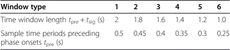
frequency range 3.0 to 15.0 Hz. Such a wide frequency range was selected in order to avoid cycle skipping and because, on the ocean bottom, seismic noise tends to be low in this frequency band (e.g., Walker 1984; Webb 1998). In addition, the length of the time windows was chosen so as to exclude S-wave onsets from the time windows for P-waves. Hereafter, these 3-s-long time windows are referred to as ‘parent’ time windows. From these parent time windows, six shorter ‘child’ time windows were selected, as shown in Table 1. These child time windows had different lengths and were used to perform CC measurements. Although all the OBSs were equipped with three-component velocity sensors, we used only the vertical component in the present study. That is
because it was found that the S-waves of the horizontal components were more subject to cycle skipping than those of the vertical components.
CC calculation using different window lengths
To calculate the CCs, the algorithm reported by Schaff and Waldhauser (2005), which is based on the use of a correlation detector, was employed. A variant of the cross-correlation function, CC(τ), was calculated by sliding the seismogram of a child time window over a different parent time window, namely
CCð Þ ¼τ X for the parent and child time windows, respectively, and
τ denotes the delay time. Both seismograms y1(t) and
y2(t) are aligned using the manual arrival time pick at
LS01
134˚E 135˚E 136˚E
33˚N
34˚N Shikoku Island Kii Peninsula
PH PA
01 07 01 07 01 07 01 07
2004 2005 2006 2007
Date
2nd 3rd 4th 5th
(a)
(b)
Nankai Trough
Figure 1Study area and observation periods. (a)Study area and station distribution. The yellow circles and red squares show the location of OBSs and on-land stations, respectively. OBS names are also shown. The black dashed line depicts the Nankai Trough. The location of the study area is shown in the inset map with a red rectangle. PA and PH in the inset map represent the Pacific Plate and the Philippine Sea Plate, respectively. (b)Observation periods for each OBS station. The colored horizontal bars show the periods of available data at each station. The locations of OBS stations along the vertical axis are presented in Figure 1a.
Table 1 Time lengths of six types of child time windows
Window type 1 2 3 4 5 6
Time window lengthtpre+tsig(s) 2 1.8 1.6 1.4 1.2 1.0 Sample time periods preceding
phase onsetstpre(s)
t= 0. The time range for the summations in Equation1
is the same as that for the child time windows, and tpre andtsigrepresent the sample time periods preceding and succeeding the arrival time (t= 0), respectively. From the CC(τ) values calculated in this way, the maximum CC is given by
CCmax ¼ max CC½ ð Þτ ; ð2Þ
and the corresponding delay time is written asτmax,
CCðτmaxÞ ¼CCmax ð3Þ
To avoid cycle skipping, we repeated the above CC calculations with different child time window lengths (Table 1) and extracted only stable results using the fol-lowing procedure:
For two given seismograms A and B, CC
measurements were performed six times using the parent time window for seismogram A and the six child time windows for seismogram B. The resulting
CCs and delay times are referred to as CCð Þmaxi and
τð Þmaxi respectively (i= 1, 2,…, 6).
These calculations were then repeated following
switching of seismograms A and B, which yielded six
additional sets of CCð Þmaxi andτð Þmaxi ði¼7;8;…;12Þ.
If the conditions
max s ið Þτð Þmaxi −s jð Þτð Þmaxj
h i
i≠j≤0:02 secð Þ; s ið Þ ¼ −11 ððii¼¼17;; 28;;……;;612ÞÞ
ð4Þ
were satisfied, the measurements were regarded as stable, and the results obtained using a 2-s-long child time window were used.
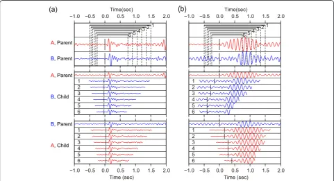
Figure 2 shows examples of accepted and rejected measurements using this procedure.
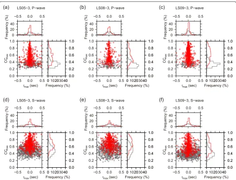
We evaluated the effectiveness of the above method by applying it to closely located source pairs in the hy-pocenter list of Akuhara et al. (2013), whose hypocen-ter separation was less than 5 km. Figure 3 shows both accepted and rejected results for three OBSs (LS05-3, LS08-3, and LS09-3) for both P- and S-waves. The ac-cepted results are centered on τmax= 0, which indicates the consistency of the manual arrival time picks. For S-waves, the acceptedτmaxvalues are more scattered about
τmax= 0 than those for P-waves. This implies that the
−1.0 −0.5 0.0 0.5 1.0 1.5 2.0
Time(sec)
1 2 3 4 5 6
1 2 3 4 5 6
−1.0 −0.5 0.0 0.5 1.0 1.5 2.0
Time (sec) 1
2 3 4 5 6
−1.0 −0.5 0.0 0.5 1.0 1.5 2.0
Time(sec)
1 2 3 4 5 6
1 2 3 4 5 6
−1.0 −0.5 0.0 0.5 1.0 1.5 2.0
Time (sec) 1
2 3 4 5 6 A, Parent
B, Parent
B, Parent
A, Parent
B, Child
A, Child
(a)
(b)
manual pick values are less accurate for S-waves, prob-ably because of contamination by the P-wave coda at the S-wave onset.
In Figure 3, it can also be seen that the rejected results tend to have low CCmaxvalues and more scattered about
τmax= 0 than the accepted ones. This is considered to be because these phase pairs are so dissimilar that the max-imum correlation does not always occur at the phase on-sets. In contrast, the rejected S-wave results for LS05-3 and LS08-3 tend to have high CCmaxvalues (>0.6). This is believed to be due to the dominance of a specific range of frequencies in the spectra of S-waves due to the presence of unconsolidated sediments beneath these OBSs, which gives rise to cycle skipping. For LS09-3, the S-wave results appear to be free from such tendencies, which suggests that there are different site effects at this station than at LS05-3 and LS08-3. Note that the OBS positions were close to each other, and the observation
periods were identical, so almost the same set of earth-quakes was used at each station in the above analysis.
For each OBS, we applied the algorithm to earthquake pairs with hypocenter separations of less than 75 km. The number of input phase pairs was about 8.5 million, from which about 2.4 million results were accepted using the above process. In addition, we also applied the method to about 17.0 million phase pairs recorded by OBS pairs at the same sites, but for different observation periods (LS01-1 and LS01-2, for example) to acquire about 4.4 million accepted results. In the following analysis, only the accepted results are used.
CC thresholds
The next task was to determine the threshold for CCmax, which should vary from one OBS to another due to site effects. CCmax represents the degree of similarity bet-ween two phases with respect to the source terms (focal
0.0
0.0 Hypocenter separation (km)
LS05−3, P−wave Hypocenter separation (km)
LS08−3, P−wave Hypocenter separation (km)
LS09−3, P−wave Hypocenter separation (km) LS09−2, LS09−3, P−wave
30% 50% Hypocenter separation (km)
LS05−3, S−wave Hypocenter separation (km)
LS08−3, S−wave Hypocenter separation (km)
LS09−3, S−wave Hypocenter separation (km) LS09−2, LS09−3, S−wave
30% 50% 70% 90% (h)
Figure 4Relationship between CCmaxand hypocenter separation (a to h).The computed CCmaxvalues are divided into hypocenter separation bins with widths of 1 km. The cumulative frequency is then calculated for each bin. The cumulative frequency results for 30%, 50%, 70%, and 90% are plotted.
0
LS09−2, LS09−3, P−wave
n=112483
LS09−2, LS09−3, S−wave
n=45830
(h)
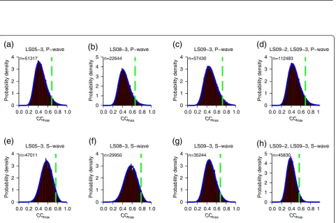
Figure 5Distributions of CCmax(a to h) for earthquake pairs with a large hypocenter separation.The red bars represent the probability
mechanisms and radiation patterns) and the propagation paths. Site effects also influence CCmax, acting as filters in the frequency domain.
We investigated the effect of the propagation path by examining the relationship between CCmaxand hypocen-ter separations between two events. All phase pairs were first divided into bins based on their hypocenter separa-tions, as determined from the hypocenter list. The cu-mulative frequency of CCmax was then calculated for each bin, which had a width of 1 km. Here, the cumu-lative frequency is defined as the percentage of CCmax values that are lower than a given value. Figure 4 shows typical results for the cumulative frequency. It can be seen that it rapidly decreases as the hypocenter separ-ation becomes more than a few kilometers and then re-mains almost constant. From these results, we assumed that the statistical distributions of CCmax at each OBS
become stable (independent of the hypocenter separ-ation) if the sources are separated by more than 30 km. By using such stable CCmaxdistributions, the bias due to the inhomogeneous source distribution can be avoided. For example, for an earthquake swarm occurring be-neath an OBS, the CCmaxdistribution will be biased to-wards higher values if closely located pairs are included.
The red histograms in Figure 5 show the CCmax distri-butions (observed probability density) for source pairs separated by more than 30 km. It is considered that the differences between the P- and S-wave distributions for the same OBS reflect differences in the radiated energy spectrum for the sources, whereas differences among OBSs are most likely due to site effects. Therefore, we used these distributions to determine the CCmax thresh-old for each OBS.
The distributions shown in Figure 5 are non-Gaussian in that they have asymmetric lobes. However, we found that they were well described using a generalized ex-treme value (GEV) distribution (Jenkinson 1955), which is a statistical distribution of the maximum values of random samples from an arbitrary probability density function. The blue curves in Figure 5 represent GEV fits to the CCmaxdistributions using the L-moment method (Hosking 1990). The CCmaxthreshold can then be deter-mined as the p-th percentile of the fitted GEV distribu-tion, which represents the value of CCmaxfor which the cumulative frequency becomes p%. The p value can be chosen in accordance with the study objectives.
The different observation periods (Figure 1b) must also be taken into consideration. Site effects are thought to be different among observation periods, even if the locations are almost the same, because different conditions exist for the mechanical coupling between the OBS and the sea-floor each time an OBS is deployed. To account for this, we determined the thresholds for all combinations of observation periods in the manner described above (Figures 4d,h and 5d,h).
900 1000 1100 1200 1300 1400 1500 1600 1700
# of clustered events
60 65 70 75 80 85 90 95 100
p value
250 255 260 265 270 275 280 285 290 295
# of clusters
cluster clustered event
Figure 6Statistical results for cluster analysis with variousp values.The open and filled circles denote the number of clusters and clustered earthquakes, respectively. The dashed line is drawn at p= 95, which was selected for this study.
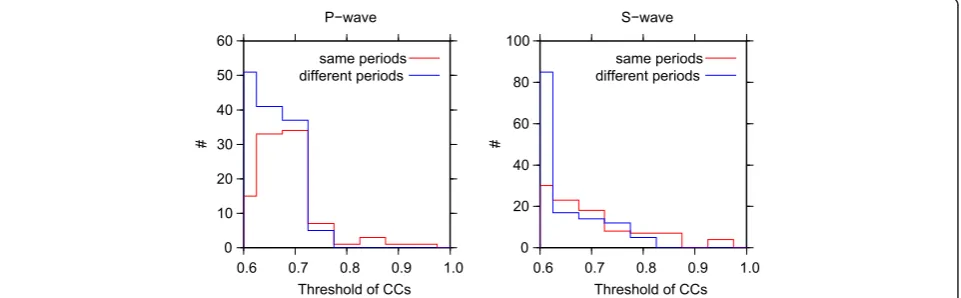
0 10 20 30 40 50 60
#
0.6 0.7 0.8 0.9 1.0 Threshold of CCs
P−wave
same periods different periods
0 20 40 60 80 100
#
0.6 0.7 0.8 0.9 1.0 Threshold of CCs
S−wave
same periods different periods
Cluster analysis of earthquakes
We next performed a cluster analysis based on the CCs in order to identify characteristic patterns in the hypo-centers around the Kii Peninsula. We defined clusters of similar earthquakes based on hypocenter separations and waveform similarities. First, any two events satisfying the following conditions were linked together: (1) the
hypocenter separation was less than 5 km, and (2) CCmax was greater than or equal to the threshold value for three or more phase pairs, including at least one S-wave pair. The linked earthquakes were then grouped into clusters using the following simple rule: if earthquakes A and B are linked and if B and C are also linked, then A, B, and C are included in the same cluster irrespective of Table 2 Conditions for double-difference hypocenter relocation
Phase Station type Number Root mean square of travel time
residuals after relocation (s)
Events - - 1,284
-Absolute travel time P On-land stations and OBSs 75,769 0.078
S 109,616 0.103
Differential travel time from hypocenter list P On-land stations and OBSs 75,536 0.052
S 123,236 0.080
Differential travel time from CC measurements P OBSs 5,036 0.017
S 12,509 0.020
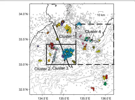
134.5˚E 135.0˚E 135.5˚E 136.0˚E
32.5˚N 33.0˚N 33.5˚N
34.0˚N 10 km
Cluster 1
Cluster 2 Cluster 3
Cluster 4
A
B
the waveform similarity between A and C. The CCmax thresholds were determined for a given p value in the manner described above. However, if the calculated threshold was lower than 0.6, it was changed to 0.6 because we noticed that waveforms began to appear dissimilar below this value.
Figure 6 shows thepvalue dependence of the number of clusters and component earthquakes. Both are seen to decrease with increasingp. Note that the lower limit for the number of clusters is determined by the maximum hypocenter separation (5 km) and the minimum CCmax threshold value (0.6). Otherwise, one large cluster contain-ing all events would be produced at an extremely low p value. When selecting the appropriate value ofp, there is a trade-off between the number of clusters and clustered events, and the CCmaxthreshold. In the present study, ap value of 95 was chosen, since this is where the two num-bers begin to drop rapidly as shown in Figure 6. Figure 7 shows the histograms of the obtained thresholds.
We then relocated the hypocenters of the linked earth-quakes using the cross-correlation results in order to im-prove the accuracy of their relative positions. This was performed by means of the double-difference algorithm (Waldhauser and Ellsworth 2000) using the tomoDD pro-gram (Zhang and Thurber 2003), which supports 3D vel-ocity structures. The 3D P- and S-wave velvel-ocity model used was obtained from a previous tomographic analysis (Akuhara et al. 2013). As input data for tomoDD, we used the differential travel time calculated from τmax, in ad-dition to the absolute and differential travel times from the hypocenter list. Additional information concerning the relocation process is listed in Table 2. In spite of the use of CC delay times, there was no remarkable change in appearance following relocation. This may be due to the relatively small number of differential travel times from the CC measurements. The root mean square values of the differential travel time residuals from the CC measurements were 0.017 and 0.020 s for and S-waves, respectively. If it is assumed that the P-and S-wave velocities are 7.0 P-and 3.8 km/s, respectively, which are actually somewhat larger than typical values for the oceanic crust, the relative location error can be estimated to be about 100 m.
Results and discussion
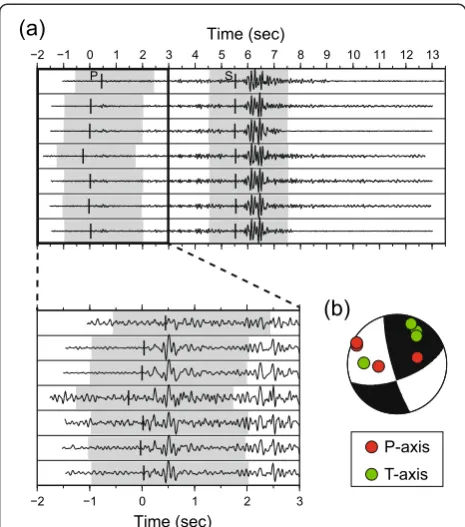
As a consequence of the cluster analysis, we obtained 278 clusters and 1,284 clustered earthquakes from a total of 4,523 earthquakes. Figure 8 shows the 49 clus-ters that contain five or more earthquakes. Figure 9a shows seismograms for the earthquakes in cluster 1 in Figure 8; it can be seen that they are extremely similar.
To investigate the characteristics of each cluster, we determined the focal mechanisms from the P-wave po-larities, which were observed at OBSs, on-land stations,
or both, using the FPFIT program (Reasenberg and Oppenheimer 1985). We accepted focal mechanisms only if they were determined from eight or more P-wave polarities, observed at stations whose maximum azimuthal gap from the hypocenter was less than 180°. A total of 541 focal mechanisms were acquired in this manner, for which the average half width of the 90% confidence region for the strike, dip, and rake was 6°, 7°, and 9°, respectively. Figure 9b shows the P- and T-axes of the focal mecha-nisms for cluster 1. Unlike the case for the waveforms themselves, large differences are observed, even if the un-certainties are taken into account. This may be caused by misidentification of the P-wave onsets or polarities due to a low signal-to-noise ratio in the OBS records. Although individual focal mechanisms are not sufficiently reliable, useful information concerning the tectonics can be ex-tracted by gathering them within each cluster.
NNE-trending faults within the oceanic mantle
Figure 10 shows an enlarged view of clusters 2 and 3 in Figure 8, located offshore to the southwest of the Kii Peninsula, which are seen to be aligned along the NNE
−2 −1 0 1 2 3
Time (sec)
−2 −1 0 1 2 3 4 5 6 7 8 9 10 11 12 13
Time (sec)
P S
(a)
(b)
P-axis
T-axis
direction. A comparison with the velocity structure mo-del obtained in a previous tomographic analysis (Akuhara et al. 2013) reveals that these earthquakes occurred within the oceanic mantle. The P- and T-axes are oriented along the directions normal and parallel to the through, respect-ively (Figure 10). These axes are consistent with the re-gional stress field, which is considered to be due to slab pulling beneath Kyushu Island and the resistance of the mantle to the subduction motion (Wang et al. 2004). The strike for each focal mechanism almost agrees with the cluster alignment direction. As shown in Figure 11, it was also found that the clusters form the lower plane of a double seismic zone, separated from the upper plane by a distance of about 15 km.
Clear lineation of earthquakes has often been inter-preted as being associated with faults, on the basis of add-itional geological evidence (e.g., Waldhauser et al. 1999). Unfortunately, in the present case, no geological evidence is available that directly supports the existence of faults, 134.6˚E 134.7˚E 134.8˚E 134.9˚E 135.0˚E 135.1˚E 135.2˚E 135.3˚E
33.0˚N 33.1˚N 33.2˚N 33.3˚N 33.4˚N
5 km
0
10
20
30
40
Depth (km)
134.6˚E 134.7˚E 134.8˚E 134.9˚E 135.0˚E 135.1˚E 135.2˚E 135.3˚E Longitude
33.0˚N 33.1˚N 33.2˚N 33.3˚N 33.4˚N
Latitud
e
0 10 20 30 40
Depth (km) Cluster 2
Cluster 3
Figure 10Hypocenter distribution of NNE-trending linearly aligned clusters (clusters 1 and 2).The same symbols and colors are used for earthquake clusters with five or more earthquakes as those in Figure 8. The gray dashed lines in the cross sections represent the plate interface and the oceanic Moho estimated by a previous tomography analysis (Akuhara et al. 2013). The locations of the cross sections are represented by black dashed lines. Focal mechanisms are shown using the same notation as in Figure 9b. The arrows indicate the lineation directions for the earthquake clusters.
B A
0
20
40
Depth (km)
0 20
40 60
80 100
Distance (km)
North South
Cluster 3
because of the difficulty of offshore exploration at the depths involved. However, the geological features of the shallow part of the Philippine Sea slab can be helpful in placing some constraints on the cause of cluster lineation. Tsuji et al. (2013) conducted reflection seismic surveys seaward of the Nanakai Trough, off the Kii Peninsula, to identify a fault network within the oceanic crust, where some of the faults cross the Moho to the upper mantle. The fault network is similar to the clusters in the present study in that both comprise a sequence of parallel linea-ments. In addition, the NNE trend of the lineaments is dif-ferent from that of the fossil spreading axis of the Shikoku Basin with a NW-SE strike (Okino et al. 1994; Kido and Fujiwara 2004), along which faulting is expected to occur easily. This falsifies the hypothesis that the faults were formed long after subduction began, because once the slab has been subducted to a certain depth, the only possible mechanism for creating such a large fault is by trough-parallel regional tension. However, such tension is more likely to produce NW-SE faults along the direction of the fossil spreading axis. Consequently, it is considered that the earthquake clusters represent preexisting faults that were formed before subduction occurred.
It is well established that faults act as conduits in the outer trench regions, allowing fluids to seep into the man-tle, and promote its serpentinization (e.g., Ranero et al.
2003; Faccenda et al. 2009). The serpentinized mantle dehydrates under certain conditions of temperature and pressure to cause intraslab earthquakes by overcoming the high confining pressure, which is a plausible explanation for the double seismic zones (Hacker 2003). Yamasaki and Seno (2003) calculated the temperature structure beneath the Kii Peninsula, and demonstrated that dehydration of the metamorphosed crust and serpentinized mantle could lead to upper and lower planes, respectively. The expected separation of the two planes is approximately 10 to 20 km, which is consistent with the results obtained in the pre-sent study. Therefore, it can be concluded that these clustered earthquakes occur due to dehydration of the serpentinized mantle along preexisting faults. Miyoshi and Obara (2010) also reported the existence of a lower plane at the northeastern part of the Kii Peninsula and con-cluded that it is the result of slab bending. However, on the basis of the number of earthquakes and the separation between the upper and lower planes, the lower plane iden-tified by Miyoshi and Obara (2010) is considered to have a different origin to that in the present study.
Interplate earthquake cluster
As shown in Figures 8 and 12, cluster 4 at the southern tip of the Kii Peninsula contains more than 30 earth-quakes with a low-angle thrust-fault focal mechanism.
135.4˚E 135.6˚E 135.8˚E 136.0˚E 136.2˚E
33.0˚N 33.2˚N 33.4˚N 33.6˚N 33.8˚N
5 km
0
10
20
30
40
Depth (km)
135.4˚E 135.6˚E 135.8˚E 136.0˚E 136.2˚E
Longitude
33.0˚N 33.2˚N 33.4˚N 33.6˚N 33.8˚N
Latitude
0 10 20 30 40
Depth (km) Cluster 4
(a)
(b)
01 07 01 07 01 07 01 07
2004 2005 2006 2007
Date
35
5
15
5
5
6
5
9
8
23
12
7
6
6
7
The magnitude range is from 1.0 to 3.4. By comparing the velocity structure model and the convergence direc-tion of the PHS plate, it can be concluded that these earthquakes occur at the plate interface. Focal mecha-nisms for neighboring clusters are also shown in Figure 12, revealing that interplate earthquakes are specific charac-teristic of cluster 4. Note that the cluster indicated by lime circles also has a low-angle thrust focal mechanism, but it is located within the oceanic crust. In addition, compared to the other clusters, cluster 4 is characterized by a large number of earthquakes and long periods of seismic ac-tivity (Figure 12b).
The repeated occurrence of similar earthquakes on the plate interface has been interpreted as slip at localized as-perities (Igarashi et al. 2003). Kodaira et al. (2006) discov-ered a high-density rock body embedded in the overriding plate at almost the same location as the interplate clus-ters, although its center is shifted slightly southeastward (Figure 12). They estimated the excess normal stress to be more than 30 MPa, taking account of the results obtained from gravity observations (Honda and Kono 2005), which suggests that the embedded rock is a strong asperity at the plate interface. Moreover, the rate of interplate coup-ling drastically changes at the northeastern edge of the rock body: the coupling rate is higher seaward and lower landward (Miyazaki and Heki 2001; Saiga et al. 2011). Hence, it is considered that both sides of the plate in-terface are strongly coupled due to the weight of the rock body, with the strain being concentrated at the northwestern edge, where the interplate cluster is located. Long-term observations of these interplate earthquakes might provide insights into the process of strain accumu-lation during interseismic periods, which leads to mega-thrust earthquakes.
Conclusions
In the present study, CC results for records obtained by OBSs deployed off the Kii Peninsula were used to carry out a cluster analysis of earthquakes. We proposed me-thods to deal with problems intrinsic to OBS data, namely the predominance of monotone frequencies and varying site effects among stations. These methods involved mul-tiple CC calculations, using time windows with different lengths, and appropriately determining the CC threshold, which varied among OBSs. By applying the appropriate threshold, we identified clusters of similar earthquakes.
There was found to be two types of characteristic clus-ters. The first existed within the oceanic mantle and was aligned along the NNE direction, forming the lower plane of a double seismic zone. This is considered to represent a preexisting fault formed before subduction began. It is proposed that these earthquakes are the result of dehy-dration of the serpentinized mantle along this fault. The second finding is a cluster of interplate earthquakes at
the southern tip of the Kii Peninsula. We proposed that the primary generation mechanism for earthquakes in this cluster is strain accumulation beneath a high-density rock body.
The tectonics of most ocean areas remains unclear. We believe that the proposed method can be easily applied to OBS data from other areas, allowing new insights into the surrounding tectonics to be obtained.
Competing interests
The authors declare that they have no competing interests.
Authors’contributions
TA performed the entire analysis and drafted the manuscript. KM participated in the acquisition of data and the design of the study, and helped to draft the manuscript. Both authors read and approved the final manuscript.
Acknowledgements
We thank Kazuo Nakahigashi, Tomoaki Yamada, Masanao Shinohara, Shin'ichi Sakai, Toshihiko Kanazawa, Kenji Uehira, and Hiroshi Shimizu for collecting and processing the OBS data. This research was supported by a grant from the Global COE Program,‘From the Earth to“Earths”,’Observation and Research Program for Prediction of Earthquakes and Volcano Eruptions, and JSPS KAKENHI Grant Number 26-10221, all from the Ministry of Education, Culture, Sports, Science and Technology of Japan. General Mapping Tools (Wessel and Smith 1991) was used for drawing figures. We are grateful to two anonymous reviewers for the thoughtful comments and suggestions.
Received: 7 March 2014 Accepted: 18 July 2014 Published: 30 July 2014
References
Akuhara T, Mochizuki K, Nakahigashi K, Yamada T, Shinohara M, Sakai S, Kanazawa T, Uehira K, Shimizu H (2013) Segmentation of the Vp/Vs ratio and low-frequency earthquake distribution around the fault boundary of the Tonankai and Nankai earthquakes. Geophys Res Lett 40:1306–1310, doi:10.1002/grl.50223
Ando M (1975) Source mechanisms and tectonic significance of historical earthquakes along the Nankai Trough, Japan. Tectonophysics 27:119–140, doi:10.1016/0040-1951(75)90102-X
Baisch S, Ceranna L, Harjes HP (2008) Earthquake cluster: what can we learn from waveform similarity? Bull Seismol Soc Am 98:2806–2814, doi:10.1785/ 0120080018
Cattaneo M, Augliera P, Spallarossa D, Lanza V (1999) A waveform similarity approach to investigate seismicity patterns. Nat Hazards 19:123–138, doi:10.1023/A:1008099705858
Faccenda M, Gerya TV, Burlini L (2009) Deep slab hydration induced by bending-related variations in tectonic pressure. Nat Geosci 2:790–793, doi:10.1038/ ngeo656
Ferretti G, Massa M, Solarino S (2005) An improved method for the recognition of seismic families: application to the Garfagnana-Lunigiana Area, Italy. Bull Seismol Soc Am 95:1903–1915, doi:10.1785/0120040078 Geller RJ, Mueller CS (1980) Four similar earthquakes in central California.
Geophys Res Lett 7:821–824, doi:10.1029/GL007i010p00821
Hacker BR (2003) Subduction factory 2. Are intermediate-depth earthquakes in subducting slabs linked to metamorphic dehydration reactions? J Geophys Res 108:2030
Honda R, Kono Y (2005) Buried large block revealed by gravity anomalies in the Tonankai and Nankai earthquakes regions, southwestern Japan. Earth Planets Space 57:e1–e4
Hosking JRM (1990) L-moments: analysis and estimation of distributions using linear combinations of order statistics. J R Stat Soc Ser B 52:105–124 Igarashi T, Toru M, Hasegawa A (2003) Repeating earthquakes and interplate
aseismic slip in the northeastern Japan subduction zone. J Geophys Res 108:2249, doi:10.1029/2002JB001920
Kido Y, Fujiwara T (2004) Regional variation of magnetization of oceanic crust subducting beneath the Nankai Trough. Geochem Geophys Geosystems 5:Q03002, doi:10.1029/2003GC000649
Kodaira S, Hori T, Ito A, Miura S, Fujie G, Park J-O, Baba T, Sakaguchi H, Kaneda Y (2006) A cause of rupture segmentation and synchronization in the Nankai trough revealed by seismic imaging and numerical simulation. J Geophys Res 111:B09301, doi:10.1029/2005JB004030
Kodaira S, Takahashi N, Nakanishi A, Miura S, Kaneda Y (2000) Subducted seamount imaged in the rupture zone of the 1946 Nankaido earthquake. Science 289:104–106, doi:10.1126/science.289.5476.104
Lin G, Shearer P (2007) Estimating local Vp/Vs ratios within similar earthquake clusters. Bull Seismol Soc Am 97:379–388, doi:10.1785/0120060115 Miyazaki S, Heki K (2001) Crustal velocity field of southwest Japan: subduction
and arc-arc collision. J Geophys Res 106:4305–4326, doi:10.1029/ 2000JB900312
Miyoshi T, Obara K (2010) Double seismic zone within the ridge-shaped slab beneath southwest Japan. Earth Planets Space 62:949–954, doi:10.5047/ eps.2010.11.001
Mochizuki K, Nakahigashi K, Kuwano A, Yamada T, Shinohara M, Sakai S, Kanazawa T, Uehira K, Shimizu H (2010) Seismic characteristics around the fault segment boundary of historical great earthquakes along the Nankai Trough revealed by repeated long-term OBS observations. Geophys Res Lett 37:L09304, doi:10.1029/2010GL042935
Okino K, Shimakawa Y, Nagaoka S (1994) Evolution of the Shikoku Basin. J Geomagn Geoelectr 46:463–479, doi:10.5636/jgg.46.463
Ranero CR, Morgan JP, McIntosh K, Reichert C (2003) Bending-related faulting and mantle serpentinization at the Middle America trench. Nature 425:367–373, doi:10.1038/nature01961
Reasenberg PA, Oppenheimer D (1985) FPFIT, FPPLOT and FPPAGE: Fortran computer programs for calculating and displaying earthquake fault-plane solutions. US Geol Surv Open File Rep 85–739:1–109
Saiga A, Kato A, Sakai S, Iwasaki T, Hirata N (2011) Crustal anisotropy structure related to lateral and down-dip variations in interplate coupling beneath the Kii Peninsula, SW Japan. Geophys Res Lett 38:L09307, doi:10.1029/ 2011GL047405
Savage MK, Wessel A, Teanby NA, Hurst AW (2010) Automatic measurement of shear wave splitting and applications to time varying anisotropy at Mount Ruapehu volcano, New Zealand. J Geophys Res 115:B12321, doi:10.1029/ 2010JB007722
Schaff DP, Waldhauser F (2005) Waveform cross-correlation-based differential travel-time measurements at the Northern California seismic network. Bull Seismol Soc Am 95:2446–2461, doi:10.1785/0120040221
Shearer P, Hauksson E, Lin G (2005) Southern California hypocenter relocation with waveform cross-correlation, part 2: results using source-specific station terms and cluster analysis. Bull Seismol Soc Am 95:904–915, doi:10.1785/ 0120040168
Shiomi K, Matsubara M, Ito Y, Obara K (2008) Simple relationship between seismic activity along Philippine Sea slab and geometry of oceanic Moho beneath southwest Japan. Geophys J Int 173:1018–1029, doi:10.1111/ j.1365-246X.2008.03786.x
Tsuji T, Kodaira S, Ashi J, Park JO (2013) Widely distributed thrust and strike-slip faults within subducting oceanic crust in the Nankai Trough off the Kii Peninsula, Japan. Tectonophysics 600:52–62, doi:10.1016/j.tecto.2013.03.014 Waldhauser F, Ellsworth WL (2000) A double-difference earthquake location
algorithm: method and application to the northern Hayward fault, California. Bull Seismol Soc Am 90:1353–1368, doi:10.1785/0120000006
Waldhauser F, Ellsworth WL, Cole A (1999) Slip-parallel seismic lineations on the northern Hayward fault, California. Geophys Res Lett 26:3525–3528, doi:10.1029/1999GL010462
Walker DA (1984) Deep ocean seismology. Eos, Trans Am Geophys Union 65:2–3, doi:10.1029/EO065i001p00002
Wang K, Wada I, Ishikawa Y (2004) Stresses in the subducting slab beneath southwest Japan and relation with plate geometry, tectonic forces, slab dehydration, and damaging earthquakes. J Geophys Res 109:1–15, doi:10.1029/2003JB002888
Watanabe H (1971) Determination of earthquake magnitude at regional distance in and near Japan (in Japanese). J Seism Soc Jpn 24:189–200
Webb SC (1998) Broadband seismology and noise under the ocean. Rev Geophys 36:105–142, doi:10.1029/97RG02287
Wessel P, Smith WHF (1991) Free software helps map and display data. Eos Trans Am Geophys Union 72:441–441, doi:10.1029/90EO00319
Yamasaki T, Seno T (2003) Double seismic zone and dehydration embrittlement of the subducting slab. J Geophys Res 108:2212, doi:10.1029/2002JB001918 Zhang H, Thurber CCH (2003) Double-difference tomography: the method and its application to the Hayward fault, California. Bull Seismol Soc Am 93:1875–1889, doi:10.1785/0120020190
doi:10.1186/1880-5981-66-80
Cite this article as:Akuhara and Mochizuki:Application of cluster analysis based on waveform cross-correlation coefficients to data recorded by ocean-bottom seismometers: results from off the Kii Peninsula.Earth, Planets and Space201466:80.
Submit your manuscript to a
journal and benefi t from:
7 Convenient online submission 7 Rigorous peer review
7 Immediate publication on acceptance 7 Open access: articles freely available online 7 High visibility within the fi eld
7 Retaining the copyright to your article