IJISET - International Journal of Innovative Science, Engineering & Technology, Vol. 2 Issue 4, April 2015. www.ijiset.com
ISSN 2348 – 7968
1122
Band Stop optimization of Frequency Selective Surfaces Using
the Transmission Line Modeling Method
Dominic S Nyitamen1, Steve Greedy2, Christopher Smartt2 and David W P Thomas2
1. Electrical Electronic Engineering Department, NDA, Kaduna Nigeria 2. George Green Institute for Electromagnetic Research
The University of Nottingham Nottingham, NG7 2RD, UK
Keywords Optimization, shielding, Frequency selective surface, TLM, Modeling
Abstract— Optimization is applied to Transmission Line Method (TLM) modeling of a Double Square Loop Frequency Selective Surface for electromagnetic shielding in the 900MHz and 1800MHz bands. The objective function to be optimized is based on the transmission coefficients at frequencies in the stop-bands. In this work the use of GG_TLM inside an optimization process is demonstrated. It is the purpose of optimization to find the set of parameter values which best minimizes the objective function. At least 20dB return loss is required. Combining the TLM solution with an optimization technique reduces the human input required in searching for the optimal set of parameters for the dual band frequency selective surface (FSS). A good agreement is found between simulation and experimental work.
Keywords— Frequency Selective Surface, shielding, Transmission line modeling, optimize
I. INTRODUCTION
The Transmission Line Modelling (TLM) technique is a time domain numerical method that is often used to solve the differential form of Maxwell’s equations. Electromagnetic modeling techniques are employed for analyses and designs using electrical component analogy [1]. In addition to this we may use GGI_TLM to optimize designs so as to achieve or optimize a specified performance criterion. In this work the use of GG_TLM inside an optimization process is demonstrated. A specified number of parameters together with a figure of merit (objective function) for the design which is intended to minimize is chosen. It is the purpose of optimization to find the set of parameter values which best minimizes the objective function.
Frequency selective surfaces (FSS) have found widespread application from antennas to filters at microwave frequencies [2-5]. FSS are either patches or apertures arranged in a periodic fashion in a conducting surface for frequency filtering. The frequency behavior of the FSS is determined completely by the dimensions of the surface in one period or unit cell. The Transmission Line Method (TLM) [6] is used in the modeling analysis and
design of the Double Square Loop. The TLM electromagnetic solver enables losses in the dielectric substrates and the finite conductivity of the printed patches of the FSS to be accounted for. Finally, optimization is applied in the TLM using the multidimensional generalization of the bisection method for the design of Double Square Loop Frequency Selective Surface. The objective function to be optimized (minimized in this case) is based on the transmission coefficients in two stop frequency bands of (900 and 1800MHz). A return loss of at least 20dB is sought.
The paper is organized as follows: section I is the introduction, while section II presents the TLM modelling technique. Section III is the optimization scheme applied in the TLM and section IV shows the experimental setup and measurements with section V been the conclusion.
II. THE TLM METHOD
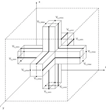
The TLM modeling technique is an explicit numerical method that is founded on the equivalence between voltages and currents on a transmission line network and electric and magnetic fields in 3D space. The 3D time domain Electromagnetic field solver creates and solves problems on a structured cubic mesh [6].
The boundary description of symmetrical condensed node is easy to work with since all the six filed components can be defined at a single point in space [7]. The waves are characterized by voltage and current and their associated Electric and Magnetic fields. The Electric and Magnetic fields are orthogonal to each other and to the direction of propagation. For example a z directed transmission line polarized in the x direction is associated with the fields Ex and Hy.
ISSN 2348 – 7968
Figure 1. Symmetrical condensed node (SCN).
The problem space is discretised into cubic cells where the cell size is significantly smaller than the shortest wavelength of interest in the analysis. Each cell face has two orthogonal TEM transmission lines (link lines) with associated Electric and Magnetic field components tangential to the cell face. The transmission lines incident from each face intersect at the cell centre forming a junction.
The link transmission lines have distributed capacitance and inductance representing the permittivity and permeability of a vacuum. For materials other than free space, the permittivity or permeability may be augmented by the addition of suitably defined stub transmission lines.
A voltage impulse incident on the cell centre junction from one of the link lines scatters back into the link lines, this process is described by a scattering matrix. The scattering matrix is defined such that the transmission line network models Maxwell's equations. The scattered voltage pulses reach the cell faces half a time-step later and connect to adjacent cells. The TLM algorithm can be considered as a discrete version of Huygen’s principle [6].
The propagation delay on every transmission line in the network (the simulation time-step) is chosen to be the same. This property of the network provides discretisation in time and ensures time synchronization of the scatter and connect processes in the network.
The structure of the cell is such that all 3 components of both electric and magnetic field are evaluated at the cell centre during the scattering process and tangential Electric and Magnetic field components are calculated half a time-step later at the cell faces during the connect process.
Boundary conditions are applied on the outer surfaces of the problem space as required for the scenario under study. Boundary conditions may represent perfectly conducting surfaces or implement an absorbing boundary condition for example.
The open source TLM code GGI_TLM [10] is applied to the modeling of the dual band stop FSS. The GGI_TLM code allows the imposition of a ‘wrapping boundary condition’ [11], allowing the simulation of an infinite periodic array of elements with a model of a single cell of the FSS structure. The GGI_TLM code is a time domain method, frequency domain results are obtained by the Fourier Transform thus GGI_TLM predicts the response of the FSS over the entire frequency range of interest.
The square loops of the FSS are modeled as perfect electrical conductors. Wrapping boundary conditions are placed on the x and y boundaries. An absorbing boundary condition is imposed on the
z boundaries to absorb the scattered field. In the TLM model a Gaussian pulse plane wave whose width is chosen to cover the frequency band of interest is launched towards the FSS sheet. Time domain fields are recorded on both the reflection and transmission side of the FSS until all the significant electromagnetic interactions have taken place. This is followed by a post processing procedure which involves Fourier transformation to obtain the reflection and transmission coefficient characteristic of the design at the desired frequencies.
In this paper a double square loop FSS designed to block the GSM900 and GSM1800 frequencies is studied. The Fig.2 shows the relative spacing of elements of the double square loop FSS where Dim1 – Dim 4 are the optimization parameter values.
Fig.2 Double square loop optimization parameters (Dim1-4) of a unit cell
The initial value of these dimension were 50mm and evaluation steps of 2.5 mm.
Dim4
Dim3 Dim2
Dim1
IJISET - International Journal of Innovative Science, Engineering & Technology, Vol. 2 Issue 4, April 2015. www.ijiset.com
ISSN 2348 – 7968
III. Optimization of the FSS
The purpose of optimization is to find the set of the dimensions of the FSS geometric structure which best minimizes the objective function to achieve the specified performance criterion (the stop band transmission). The multi-dimensional optimization of the bisection method is explored by evaluating the objective function at various points surrounding a central point. The initial central point and separation of the surrounding points are specified, 880MHz and 920MHz then 1780MHz and 1820MHz at 20dB. At each stage of the optimization process a new point or set of points is derived based on the values of the objective function at the points already evaluated. The objective function is carefully chosen to achieve the desired performance. While the desirable features are promoted, the undesirable features of response are penalized [11].
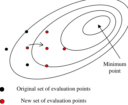
The optimization is based on a multi-dimensional generalization of the bisection method. The multi-dimensional optimization space is explored by evaluating the objective function at various points surrounding a central point. The initial central point and separation of the surrounding points must be specified by the user. At each stage of the optimization process a new point or set of points is derived based on the values of the objective function at the points already evaluated. The Figures 3 and 4 illustrate the basic operation of the bisection method in a 2D optimization space. In handling more function evaluations, the bisection method may be more efficient, and more robust in some circumstances as compared to the simplex method of optimization [10].
Fig. 3 2D optimization space
The starting point for the optimization is taken at a point from which the optimum point may be reached
by a downhill search method. Optimization of geometry: geometry definition is continuous however the resulting mesh is discrete therefore the objective function will exhibit a step-like form as a function of geometric parameters. Meshed parameters cannot be optimized beyond the mesh resolution [11].
Fig.4 convergence state
In this optimization of the dual band FSS it is required to minimize the transmission of the surface in the bands 880MHz to 920MHz and 1780MHz and 1820MHz. Some experience of working with shell scripts and Fortran programming is employed in order to achieve the optimization of parameterized models. A subroutine for the optimization code is included at the end of the paper.
Some considerations in optimisation of GGI_TLM models [10]:
The objective function should be chosen carefully so that the desired performance is achieved. It may be that undesirable features of response should be penalized as well as desirable features being promoted.
The starting point for the optimization should be at a point from which the optimum point may be reached by a downhill search method.
That the process will finds local minima of the objective function is no guarantee that this will be the global minimum. It may be useful to restart the optimization from different points so as to establish the robustness of the minimization.
Optimization of geometry: geometry definition is continuous however the resulting mesh is discrete therefore the objective function will exhibit a step-like form as a function of geometric parameters. Meshed parameters cannot be optimized beyond the mesh resolution.
Minimum point
Original set of evaluation points
New set of evaluation points
Original set of evaluation points
New set of evaluation points
m f p p e p t f T m o o f c c a t E d c C t t
The most e multi-stage pro first then movi parameters on Care mus parameters wi errors. This parameterizatio The effecti the efficiency o function with a
The most eff multi-stage p optimized fir once the opti found.
IV. The Double copper tape o consists of a 5
To conduc situated betw antennas in a then connecte E8362B mod done withou subsequently sheet. The si conical absorb
Fig.5. S2 Chamber.
A trial sim the plot is sho seen when co the optimizati
Anecho
chambe
A
efficient optimi ocess in which ing on to a refi
the coarse mes t be taken t ill lead to a v may be on of the mode iveness of the p of the optimiza a well defined
ficient optimi process in w rst then mov imum parame
MEASUREM e Square loop of paper substr 5 by 5 matrix ct measurem ween the tra an anechoic c
ed to Vector del as shown
ut the FSS measuremen ides are com rbers.
1 measurem
mulation at the own in Fig. 6 ompared with ion process.
oic
er
TX AntennaVector Ne
Analyzer
ization sequenc a coarse mesh ned mesh once sh is found. that every ch valid geometry
achieved by el.
parameterizatio ation. A smoot
minimum is de
ization sequen which a coa
ing on to a eters on the c
MENTS p FSS was ma
rate. The sam .
ments, the F ansmitting a chamber. The Network Ana
in Fig.5. Ca S sheet in nts were taken mpletely shiel
ment setup
e onset of opt 6. The improv that obtained RX Ante etwork r FSS
ce may be a h is optimized
e the optimum
hoice of tria y and cause no
y appropriate
on can affect th objective
esirable.
nce may be a arse mesh is refined mesh oarse mesh is
ade by placing mple FSS shee
FSS sheet is and receiving e antennas are alyzer (VNA) alibration was place, and n with the FSS lded with the
in Anechoic
timization and vement can be d at the end o
X enna al o e a s h s g t s g e ) s d S e c d e f
Fig. 6 paramete
Fig. 7 transmis using GG obtained Fig.7. S2 Measure Overa results b and me centered and mea with the dependen width. T frequenc between second dimensio However inefficien especiall some eff efficienc evaluatio S21 dB
6 TLM simul ers
7 shows a p sion coefficie G_TLM at th d with measure
21 for optimiz ements
ll there is etween the m easurements.
on f1 (904.6
asurements. W GG_TLM m nt on the inne There is howev
cy of the seco the GGI_T resonance is ons of the inn
r, the optim nt when co ly for well be fort could use cy of the
on of the ‐40 ‐35 ‐30 ‐25 ‐20 ‐15 ‐10 ‐5 0 5 0
lation with in
plot of the m ent in dB ver he end of opt
ements.
zed FSS in GG
reasonable a modeling with
The first tr MHz) for op We observe method that thi
er square side ver some diff nd resonance TLM and me
s determined er square. mization meth
ompared to ehaved objec efully be put i optimization objective 500 1000 Frequ ISSN 2348 nitial optimiz
magnitude o rsus frequenc timization and GI_TLM and agreement in GG_TLM m ransmission ptimized GG_ from simula is resonance i e length than ference seen i
at f2 (1.7812
easurements. d mainly by
hod employe other techn tive function into improvin method as functions 0 1500
ency [MHz]
IJISET - International Journal of Innovative Science, Engineering & Technology, Vol. 2 Issue 4, April 2015. www.ijiset.com
ISSN 2348 – 7968
1126
GGI_TLM may be very time consuming. The method used here is only suitable for problems which can be simulated in a matter of minutes or at most hours.
V. CONCLUSION
It is demonstrated in this work that optimization can be applied in GGI_TLM for optimum designs of frequency selective surfaces. The shielding effectiveness of the double square loop achieved in this study is in excess of 25dB at 900MHz and at 1,800MHz. The good agreement between the simulated and experimental results shows that GG_TLM can be used to model FSSs with double square loop patch elements for shielding. Optimization applied in the GG_TLM provides a robust means of arriving at the premium set of parameters for the design.
OPTIMIZATION SUBROUTINE IMPLICIT NONE
real*8 :: value
real*8 :: cell_size,dim1,dim2,dim3,dim4 real*8 :: t1,t2,t3,t4
real*8 :: r(9) integer :: i,ii integer :: nvalues
! START
! set the FSS dimensions from the parameter ! values
t1=4e-2*parameters(1) t2=1e-2*parameters(2) t3=2e-2*parameters(3) t4=2e-2*parameters(4)
dim4=t1 dim3=t1+t2 dim2=t1+t2+t3 dim1=t1+t2+t3+t4
cell_size=t1+t2+t3+t4+2e-2*parameters(5)
! evaluate the function to minimize
! First write the dimensions to a file open(unit=50,file='FSS_dimensions')
write(50,8000)cell_size,dim1,dim2,dim3,dim4 8000 format(5E16.6)
close(unit=50)
! Run the script which runs and post processes the TLM solution
CALL system("run_GGI_TLM_FSS_solution run_seq OPTIMISE_FSS")
! Calculate the objective function to optimise from the output result(s)
value=0d0
open(unit=50,file='S21.fout') ! read header line
read(50,*)
! read the data file nvalues=0
1000 CONTINUE
read(50,*,end=1010)(r(ii),ii=1,9)
if ( (r(1).GE.880E6).AND.(r(1).LE.920E6) ) then
value=value+r(9) ! sum the transmission coefficient in dB
nvalues=nvalues+1 else if (
(r(1).GE.1780E6).AND.(r(1).LE.1820E6) ) then value=value+r(9) ! sum the transmission coefficient in dB
nvalues=nvalues+1 end if
GOTO 1000
1010 CONTINUE
if (nvalues.EQ.0) then value=large
else
value=value/nvalues
end if
close(unit=50)
END SUBROUTINE calculate_function
REFERENCES
[1] C. Christopoulos, The transmission-line modeling method: TLM. Institute of Electrical and Electronics Engineers, 1995.
[2] Marcuvitz, Microwave Handbook Editors
McGraw-Hill, Nova Iorque, 1951
[3] B.A. Munk Frequency Selective Surfaces
Theory and Design Wiley-Interscience Publication John Welley & Sons, Inc. Canada 2000.
[4] K.R. Jha, G. Singh and R. Jyoti “A simple synthesis technique of single-square-loop frequency selective surface” Progress in Electromagnetic Research B, 2012 Vol. 45, 165-185.
[5] E.A. Parker “The gentleman’s guide to
frequency selective surfaces” 17th Q.M.W. Antenna symposium,1991, London.
[6] C. Christopoulos, “The Transmission Line
Modelling Method: TLM”, Piscataway, NY, IEEE Press, 1995.
[7] N. Komjani Barchloui and M. Solaimani
“Simulation of frequency selective surfaces using 3D transmission line matrix” Iranian Journal of Science and Technology, Transaction B, Vol. 28, No. B3, 2004.
[8] P.B. Johns “A symmetrical condensed node for
TLM method.” IEEE Trans. Microwave Theory and Tech. MIT-35, 370-377, 1987.
[9] E. Tong and Y. Fujino. An efficient algorithm
for transmission line matrix analysis of electromagnetic problems using symmetrical condensed node. IEEE Trans. Microwave Theory and Tech. MIT-35, 370-377, 1991.
[10] GGI_TLM open source TLM code:
www.girhub.com/ggiemr/GGI_TLM/
[11] GGI_TLM user documentation