Quantifying Degradation in Ceramic Matrix Composites Through Electromagnetic Interrogation and the Related Estimation Techniques.

(1)

ABSTRACT

CATENACCI, JARED WILLIAM. Quantifying Degradation in Ceramic Matrix Composites Through Electromagnetic Interrogation and the Related Estimation Techniques. (Under the direction of Dr. Harvey Banks.)

Reflectance spectroscopy obtained from thermally treated silicon nitride carbon based ceramic matrix composites is used to quantity the oxidation products SiO2 and SiN. The data collection is described in detail in order to point out the potential biasing present in the data processing. A probability distribution is imposed on selected dielectric model parameters, and then non-parametrically estimated. A non-parametric estimation is chosen since the exact composition of the material is unknown due to the inherent heterogeneity of ceramic composites. The probability distribution is estimated using the Prohorov metric framework (PMF) in which the infinite dimensional optimization is reduced to a finite dimensional optimization using an approximating space composed of linear splines. A weighted least squares estimation is carried out, and uncertainty quantification is performed on the model parameters. Our estimation results indicate a distinguishable increase in the SiO2 present in the samples which were heat treated for 100 hours compared to those treated for 10 hours.

To establish probability measure estimation in a nonparametric model using the Prohorov Metric Framework, we first summarize the computational methods and related convergence results that were recently developed by our group. Results are presented on the bias and the variance due to the approximation and the pointwise asymptotic normality of the approximated probability measure estimator is established. We propose use of a model selection criterion to balance the bias and the variance, and compare the pointwise confidence bands constructed using the asymptotic normality results with that obtained by Monte Carlo simulations. Additionally, we propose a method in which the information provided by difference based approximations of the measurement errors is used as a way of determining the presence of statistical model discrepancy. A number of numerical examples are given to illustrate the effectiveness of these proposed methods.

(2)

(3)

Quantifying Degradation in Ceramic Matrix Composites Through Electromagnetic Interrogation and the Related Estimation Techniques

by

Jared William Catenacci

A dissertation submitted to the Graduate Faculty of North Carolina State University

in partial fulfillment of the requirements for the Degree of

Doctor of Philosophy

Applied Mathematics

Raleigh, North Carolina 2016

APPROVED BY:

Dr. Amanda Criner Technical Consultant

Dr. Kevin Flores

Dr. Shuhua Hu Dr. Gerald LeBlanc

Dr. Ralph Smith Dr. Harvey Banks

(4)

DEDICATION

(5)

BIOGRAPHY

(6)

ACKNOWLEDGEMENTS

I would like to thank my advisor and friend H.T. Banks for his continual encouragement and support. A very special thanks to Shuhua Hu, who patiently provided careful guidance and through her example set a standard to aspire toward in my own career. Thanks also to the many people who early in my academic career guided and inspired me as a student and young researcher, in particular, Gabriella Pinter, Istvan Lauko, and Sarah Patch.

(7)

TABLE OF CONTENTS

LIST OF TABLES . . . .viii

LIST OF FIGURES . . . x

Chapter 1 Introduction . . . 1

1.1 Motivation . . . 1

1.2 Problem Description . . . 3

1.2.1 Reflection Coefficient: Perpendicular Polarization . . . 4

1.2.2 Reflection Coefficient: Parallel Polarization . . . 6

1.2.3 Reflection Coefficient Between Free Space and a Lossy Material . . . 7

1.2.4 Complex Permittivity . . . 8

Chapter 2 The Prohorov Metric . . . 9

2.1 Introduction . . . 9

2.2 Theoretical and Computational Framework for Probability Measure Estimation . 11 2.2.1 Consistency of the Probability Measure Estimator . . . 13

2.2.2 Approximation Schemes for Probability Measure Estimation . . . 14

2.2.3 Bias and Variance in Probability Measure Estimation . . . 16

2.2.4 Pointwise Asymptotic Normality of the Approximatd Probability Measure Estimator . . . 18

2.3 Numerical Results . . . 20

2.3.1 Optimal Value ofM . . . 21

2.3.2 Pointwise Confidence Band . . . 22

2.4 Concluding Remarks and Future Research Questions . . . 26

Chapter 3 Use of Difference-Based Methods to Explore Statistical and Math-ematical Model Discrepancy in Inverse Problems . . . 27

3.2 Difference-Based Methods . . . 33

3.3 Application on Determining an Appropriate Statistical Model . . . 35

3.3.1 Numerical Results for Simulated Data Sets . . . 35

3.3.2 Numerical Results for Experimental Data Sets . . . 47

3.4 Application on Detecting Mathematical Model Misspecification and Bootstrapping 49 3.5 Concluding Remarks and Future Research Questions . . . 55

Chapter 4 Estimation of Distributed Parameters in Permittivity Models of Composite Dielectric Materials Using Reflectance . . . 56

4.2 The Model for the Complex Dielectric Constant and the Reflection Coefficient . 56 4.3 Computational Framework . . . 58

4.3.1 Statistical Model . . . 58

4.3.2 Inverse Problem . . . 59

(8)

4.4.1 Results Obtained Using Simulated Data When Estimating a Probability

Measure on the Resonance Wavenumber . . . 61

4.4.2 Results Obtained Using Inorganic Glass Data When Estimating a Proba-bility Measure on the Resonance Wavenumber . . . 65

4.4.3 Results Obtained Using Simulated Data When Estimating a Probability Measure on the Relaxation Time . . . 70

4.5 Concluding Remarks and Future Research Efforts . . . 75

Chapter 5 Method Comparison For Estimation Of Distributed Parameters In Permittivity Models Using Reflectance . . . 77

5.2 The Model for the Complex Permittivity and the Reflection Coefficient . . . 78

5.2.1 Efimov model for permittivity . . . 78

5.2.2 Prohorov Metric Framework Model for Permittivity . . . 78

5.2.3 Reflection Coefficient . . . 79

5.2.5 Inverse Problem . . . 80

5.3 Results . . . 82

5.3.1 Simulated Data . . . 82

5.3.2 Inorganic Glass Data . . . 87

5.4 Concluding Remarks and Future Work . . . 94

Chapter 6 Quantifying the Degradation in Thermally Treated Ceramic Ma-trix Composites . . . 96

6.2 The Model for the Complex Permittivity and the Reflectance . . . 97

6.3 Interferogram to Spectrum . . . 98

6.3.1 Measurement Errors . . . 99

6.4 Inverse Problem . . . 100

6.4.2 Weighted Least Squares . . . 104

6.4.3 Uncertainty Quantification . . . 105

6.5 Results . . . 107

6.5.1 Consistency asM Increases . . . 107

6.5.2 Optimal Value ofM . . . 109

6.5.3 Comparison of Heat Treated Samples . . . 111

6.5.4 Pointwise Confidence Bands . . . 114

6.5.5 Comparison to Bootstrapping and Bayesian Estimation . . . 120

6.6 Concluding Remarks . . . 125

Chapter 7 Aggregate Data and the Prohorov Metric Framework: Efficient Gradient Computation . . . .128

7.2 Problem framework . . . 129

(9)

7.2.2 Aggregate models . . . 133

7.3 Example: Sinko-Streifer Model . . . 133

7.4 Example: Reflectance Spectroscopy Model . . . 135

7.5 Conclusions . . . 137

Chapter 8 Concluding Remarks . . . .139

(10)

LIST OF TABLES

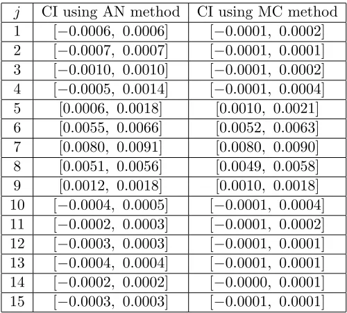
Table 2.1 The confidence intervals (CI) computed using the pointwise asymptotic normal-ity (AN) results and the ones obtained using the Monte Carlo (MC) simulations. 25 Table 3.1 Results for the logistic example in the case where γ = 0: the true value of

σ0 as well as its estimates obtained using the three mentioned methods (ˆσ1st0 is obtained using the first-order differencing method, ˆσ2nd

0 is obtained using the second-order differencing method, and ˆσ1st-3

0 is obtained by the third-order differencing method). . . 36 Table 3.2 Results for the SIR example in the case where γi = 0,i= 1,2,3: the value of

σ0,i as well as its estimates obtained using the three methods introduced in Section 3.2. . . 40 Table 3.3 The mean and standard error of the bootstrapping estimator for the logistic

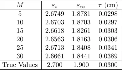
example of this section obtained using Algorithm 3.4.1 and Modified algorithm 3.4.2. . . 55 Table 4.1 Estimations obtained using the simulated data for various numbers of Dirac

measures. . . 64 Table 4.2 Estimations obtained using the reflectance data for Vitreous Germania using

various numbers of Dirac measures. . . 69 Table 4.3 Parameter estimates obtained using the reflectance data for Vitreous Silica

employing various numbers of Dirac measures compared to experimental values (abbreviated as Expt. in the table) taken from [65]. . . 74 Table 5.1 The estimated parameters using the Dirac and spline approximation methods

for the discrete distribution. . . 84 Table 5.2 The estimated values of the intensitiesSj, the relaxation timesτj, the resonance

wavenumbersk0j and the standard deviationsσj for each oscillator using the

modified Efimov approach, using the simulated data with a discrete distribution. 84 Table 5.3 The estimated parameters using the Dirac and spline approximation methods

for the simulated data with a continuous distribution. . . 85 Table 5.4 The estimated values of the intensitiesSj, the relaxation timesτj, the resonance

wavenumbers k0j and the standard deviations σj for each oscillator using

the modified Efimov approach using the simulated data with a continuous distribution. . . 87 Table 5.5 The estimated parameter values using the Dirac and spline approximation

methods to fit the Vitreous Silica data. The “true” parameter values θ0 are the experimental values taken from [65]. . . 89 Table 5.6 The estimated values of the intensitiesSj, the relaxation timesτj, the resonance

modified Efimov approach on the Vitreous Silica data. . . 89 Table 5.7 The estimated parameter values using the Dirac and spline approximation

(11)

Table 5.8 The estimated values of the intensitiesSj, the relaxation timesτj, the resonance wavenumbersk0j and the standard deviationsσj for each oscillator using the

modified Efimov approach on the data obtain from Vitreous Germania. . . . 91 Table 5.9 The estimated parameter values using the Dirac and spline approximation

methods as compared to the Efimov method to fit the Sodium Silicate Silica data. . . 93 Table 5.10 The estimated values of the intensitiesSj, the relaxation timesτj, the resonance

modified Efimov approach on the Sodium Silicate data. . . 93 Table 6.1 The estimated parameters using a data set from the 10 hour heat treated

sample 32 for M = 74 and 75. . . 108 Table 6.2 The estimated parameters using a data set from the 100 hour heat treated

sample 13 for M = 72 and 74. . . 109 Table 6.3 The estimated parameters using a data set from the 10 hour heat treated

sample 4 for M = 70,71 and 80. . . 109 Table 6.4 Estimated parameters using the first 3 locations from each sample. . . 115 Table 6.5 The 95% confidence intervals for the estimated model parameters from a

representative data set from the 10 and 100 hour heat treated samples. . . 116 Table 6.6 The 95% confidence intervals (credible intervals for the Bayesian estimation)

for the estimated model parameters from a representative data set from the 10 hour heat treated sample 32 using asymptotic theory (WLS), bootstrapping, and Bayesian estimation. . . 122 Table 6.7 The 95% confidence intervals (credible intervals for the Bayesian estimation)

(12)

LIST OF FIGURES

Figure 1.1 A monochromatic uniform wave is incident at an angleφon a plane interface between a free space and a nonmagnetic dielectric medium, where ω denotes the frequency of the wave. . . 3 Figure 2.1 Illustration of the bias and the variance in the probability measure

approxi-mation. . . 18 Figure 2.2 Illustration of the trade-off between the bias and the variance. . . 18 Figure 2.3 The AICcvalues for model (2.2.11) with M = 5,10,15,20,25 and 30. . . 23 Figure 2.4 The pointwise confidence bands for the cumulative distribution function

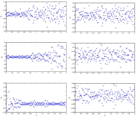
obtained using the pointwise asymptotic normality results (left) and the ones obtained using the Monte Carlo simulations (right). . . 25 Figure 3.1 Comparison of the plot of ˆε1st

j (denoted as “estimates” in the legend) versus

tj and the plot of εj (denoted as “true value”) versus tj : (left panel) results obtained forγ = 0; (right panel) results obtained for γ = 1, where ˆε1st

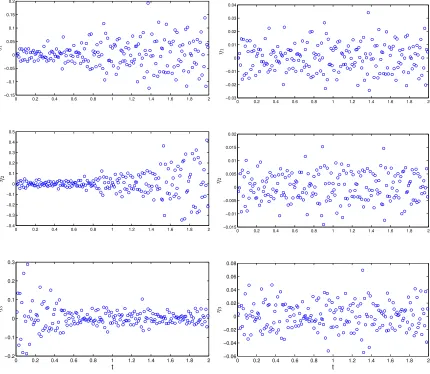
j ’s are obtained by the first-order differencing method. . . 37 Figure 3.2 Comparison of the plot of the ˆε2nd

j (denoted as “estimates” in the legend) versustj and the plot ofεj (denoted as “true value”) versus tj for the case

γ = 0 (left panel) and the caseγ= 1 (right panel), where the ˆε2nd

j are obtained using the second-order differencing method. . . 37 Figure 3.3 Comparison of the plot of the ˆε1st-3

j (denoted as “estimates” in the legend) versustj and the plot ofεj (denoted as “true value”) versus tj for the case

γ = 0 (left panel) and the case γ = 1 (right panel), where the ˆε1st-3 j are obtained by applying the first-order differencing operator for 3 times. . . 38 Figure 3.4 Plot ofη_j˜γ = ˆε1st-3

j /|yj−εˆ1st-3j |˜γ versustj for the case where the simulated data were generated with γ = 1: (left panel) ˜γ = 2; (right panel) ˜γ = 1. . . 39 Figure 3.5 Plot of η_j˜γ= ˆε2nd

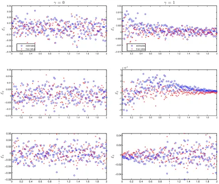
j /|yj−εˆ2ndj |γ˜ versustj for the case where the simulated data were generated with γ = 1: (left panel) ˜γ = 2; (right panel) ˜γ = 1. . . 39 Figure 3.6 Comparison of the plot of ˆε1st

ij (denoted as “estimates” in the legend) versus

tj and the plot of εij (denoted as “true value”) versus tj for the case γ1 =

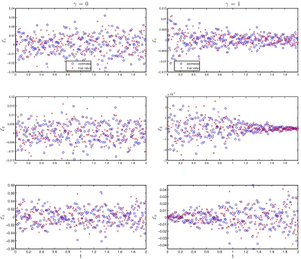
γ2 =γ3= 0 (left column) and the case γ1 =γ2=γ3 = 1 (right column). . . . 41 Figure 3.7 Comparison of the plot of ˆε2nd

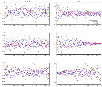
γ2 =γ3= 0 (left column) and the case γ1 =γ2=γ3 = 1 (right column). . . . 42 Figure 3.8 Comparison of the plot of ˆε1st-3

γ2 =γ3= 0 (left column) and the case γ1 =γ2=γ3 = 1 (right column). . . . 43 Figure 3.9 Plot of ηγ˜i

(13)

Figure 3.10 Plot ofη˜γi

ij = ˆε 2nd

ij /|yij−εˆij2nd|γ˜i versustj for the case where the simulated data were generated with γ1 =γ2 =γ3 = 1: (left panel) ˜γ1 = ˜γ2= ˜γ3= 2; (right panel) ˜γ1 = ˜γ2= ˜γ3 = 1. . . 46 Figure 3.11 Time plots for pseudo measurement errors obtained for the Daphnia data set

presented in [1]: (left panel) using the second-order differencing method; (right panel) using the method for applying the first-order differencing operator for three times (right). . . 47 Figure 3.12 Plots for pseudo measurement errors obtained for the CFSE data set presented

in [33, Section 3.5.3] by using the second-order differencing method: (left panel) plot of ˆεj versusj; (right panel) plot ofηγj˜ = ˆε

2nd

j /|yj−εˆ2ndj |γ˜ versus

j with ˜γ = 0.5. The vertical lines delineate the pseudo measurement errors obtained in time intervals [sk, sk+1),k= 1,2, . . . ,7. . . 48 Figure 3.13 Plots for pseudo measurement errors obtained for the CFSE data set presented

in [33, Section 3.5.3] by applying the first-order differencing operators for three times: (left panel) plot of ˆεj versus j; (right panel) plot of ηγ_j˜ = ˆ

ε1st-3

j /|yj −εˆ1st-3j |˜γ versus j with ˜γ = 0.5. The vertical lines delineate the pseudo measurement errors obtained in time intervals [sk, sk+1),k= 1,2, . . . ,7. 50 Figure 3.14 Results for fitting exponential growth model (3.4.1) to the simulated data

generated by the logistic growth model (3.3.1). . . 51 Figure 3.15 (left panel): plot of pseudo measurement errors ˆε2nd

j versustj, whereε2ndj ’s are obtained by applying the second-order differencing method to the simulated data generated by the logistic growth model (3.3.1); (right panel): residual plot (i.e., a plot of rj versustj) obtained by fitting exponential growth model (3.4.1) to the simulated data generated by logistic growth model (3.3.1). . . . 52 Figure 4.1 The model fit to the simulated data (left) and the estimated distribution of

wavenumbers (right), where the nodes are evenly placed over [405,1080] with

M = 25. . . 62 Figure 4.2 The model fit to the simulated data (left) and the estimated distribution of

wavenumbers (right), where the nodes are evenly placed over [405,1100] with

M = 25. . . 62 Figure 4.3 Model fit (left) and estimated distribution (right) where the parameters

εs, ε∞ and τ are fixed and the weights and node locations were optimized with M = 25. . . 63 Figure 4.4 Model fit (left) and the estimated distribution (right) from the full inverse

problem (4.4.3) where M = 5. . . 64 Figure 4.5 Model fit (left) and the estimated distribution (right) from the full inverse

(14)

Figure 4.9 Model fit (left) and the estimated distribution (right) from the full inverse problem (4.4.3) where M = 30. . . 67 Figure 4.10 Model fit (left) and the estimated distribution (right) from the full inverse

problem (4.4.3) where M = 5 for Vitreous Germania. . . 67 Figure 4.11 Model fit (left) and the estimated distribution (right) from the full inverse

problem (4.4.3) where M = 25 for Vitreous Germania. . . 69 Figure 4.15 The estimated distributions for all values ofM considered from the Vitreous

Germania data. . . 70 Figure 4.16 Model fit (left) and the estimated distribution (right) from the full inverse

problem (4.4.3) where M = 5 for Vitreous Silica. . . 71 Figure 4.17 Model fit (left) and the estimated distribution (right) from the full inverse

problem (4.4.3) where M = 25 for Vitreous Silica. . . 73 Figure 4.21 The estimated distributions for all values ofM considered from the Vitreous

Silica data. . . 73 Figure 4.22 Model fit (left), and the estimated distribution (right) withM = 15 fixed nodes. 74 Figure 4.23 Model fit (left) and the estimated distribution (right) where both M = 15

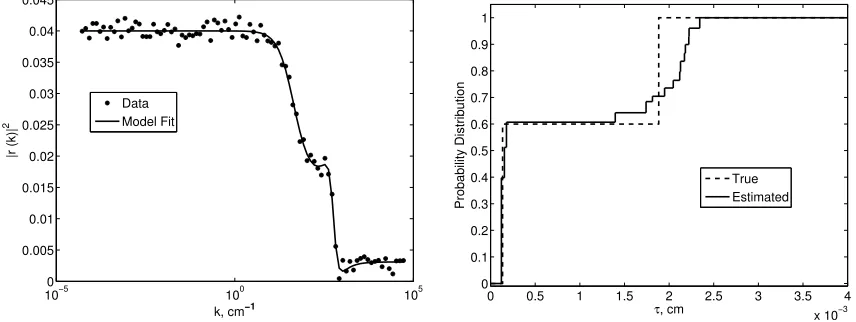
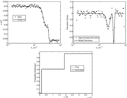
node weights and locations were optimized. . . 74 Figure 4.24 Model fit (left), the derivative of reflectance fit (right), and the estimated

distribution (bottom) where bothM = 15 node weights and locations were optimized. . . 75 Figure 5.1 The model fits to the simulated data generated with a discrete distribution.

The model fit using the Dirac approximation scheme is labeled as D45 and the spline approximation schemes as S45, where 45 is the number of nodesM, and the model fit using the modified Efimov method is labeled as E6 where

J = 6 oscillators were used. . . 83 Figure 5.2 The estimated distributions to the simulated data using a discrete distribution

using the Dirac approximation method with M = 15,25,35 and 45 nodes (left) and using the spline approximation method with M = 25,35,45 and 55

(15)

Figure 5.3 The model fits to the simulated data generated with a continuous distribution. For the Dirac and spline approximation schemes the number of nodes was taken as M = 25 (labeled as D25 and S25 respectively) and for the Efimov approach we haveJ = 2 (labeled as E2). . . 86 Figure 5.4 The estimated distributions to the simulated data using a continuous

dis-tribution using the Dirac approximation method (left) and using the spline approximation method (right). For both methods we chose the number of nodes to beM = 10,15,20 and 25. . . 86 Figure 5.5 The model fits to the Vitreous Silica data.. For the Dirac and spline

approxi-mation schemes the number of nodes was taken as M = 50 (labeled as D50 and S50 respectively) and for the Efimov approach we haveJ = 8 (labeled as E8). . . 88 Figure 5.6 The estimated distributions to the Vitreous Silica data using the Dirac

approximation method (left) and using the spline approximation method (right). For both methods we chose the number of nodes to be M = 30, 50

and 80. . . 88 Figure 5.7 The model fits to the Vitreous Germania data. For the Dirac and spline

approximation schemes the number of nodes was taken asM = 50 (labeled as D50 and S50 respectively) and for the Efimov approach we have J = 8 (labeled as E8). . . 90 Figure 5.8 The estimated distributions to the Vitreous Germania data using the Dirac

approximation method (left) and using the spline approximation method (right). For both methods we chose the number of nodes to be M = 30, 50

and 80. . . 90 Figure 5.9 The model fits to the Sodium Silicate data. For the Dirac and spline

approxi-mation schemes the number of nodes was taken as M = 25 (labeled as D25 and S25 respectively) and for the Efimov approach we haveJ = 9 (labeled as E9). . . 92 Figure 5.10 The estimated distributions to the Sodium Silicate data using the Dirac

approximation method (left) and using the spline approximation method (right). For both methods we chose the number of nodes to be M = 25 and 30. 93 Figure 6.1 Example reflectance data sets from sample 4 which was heat treated for 10

hours (the black dots) and from sample 1 which was heat treated for 100 hours (the blue circles). . . 97 Figure 6.2 Double sided, bi-directional interferogram. . . 99 Figure 6.3 Estimated measurement error, in percent reflectance, obtained when using a

zerofilling factor of 8 and averaging the spectrum from first and second ZPD. 101 Figure 6.4 Estimated measurement error obtained, in percent reflectance, when using a

zerofilling factor of 8 and using only the spectrum from first ZPD. . . 101 Figure 6.5 Estimated measurement error obtained, in percent reflectance, when using no

zero padding and using only the spectrum from first ZPD. . . 102 Figure 6.6 Estimated measurement error from a data set from Sample 1 obtained when

(16)

Figure 6.7 Plot of the weights wj (left) and ηbj =w

−1

j νbj (right) for the 100 hour heat

treated sample 1. . . 103 Figure 6.8 Using a data set from the 10 hour heat treated sample 32, the model fit to

the data (left) and the estimated density (right) usingM = 74 and 75 nodes. 108 Figure 6.9 Using a data set from the 100 hour heat treated sample 13, the model fit to

the data (left) and the estimated density (right) usingM = 72 and 74 nodes. 108 Figure 6.10 Using a data set from the 10 hour heat treated sample 4, the model fit to the

data (left) and the estimated density (right) using M = 70,71 and 80 nodes. 109 Figure 6.11 A snapshot of the AICc values using a data set obtained from the 10 hour

heat treated sample 4 withM = 70,71, ...,90. . . 112 Figure 6.12 The model fits (left) and estimated densities (right) using the first three

locations of the data obtained from the 10 hour heat treated sample 4. . . . 112 Figure 6.13 The model fits (left) and estimated densities (right) using the first three

locations of the data obtained from the 100 hour heat treated sample 13. . . 114 Figure 6.17 The estimated densities for each location from the 10 hour heat treated data

obtained from sample 4 (top left), sample 16 (top right), and sample 32 (bottom center). . . 116 Figure 6.18 The estimated densities for each location from the 100 hour heat treated data

obtained from sample 1 (left) and sample 13 (right). . . 117 Figure 6.19 The mean density for each sample. . . 117 Figure 6.20 The modified residuals versus wavenumber k (left) and versus the model

solution (right) for the 10 hour heat treated sample 32. . . 118 Figure 6.21 The modified residuals versus wavenumber k (left) and versus the model

solution (right) for the 100 hour heat treated sample 1. . . 118 Figure 6.22 The estimated density and the corresponding pointwise confidence band for a

data set obtained from the 10 hour heat treated sample 32. . . 119 Figure 6.23 The estimated density and the corresponding pointwise confidence band for a

data set obtained from the 100 hour heat treated sample 1. . . 119 Figure 6.24 Comparison of the estimated density using weighted least squares (WLS),

bootstrapping, and Bayesian estimation for a 10 hour heat treated data set from sample 1. . . 123 Figure 6.25 Comparison of the 95% confidence/credible intervals (CI) for the estimated

weights using asymptotic theory (WLS), bootstrapping, and Bayesian estima-tion for a 10 hour heat treated data set from sample 1. . . 123 Figure 6.26 Comparison of the estimated density using weighted least squares (WLS),

(17)

Figure 6.27 Comparison of the 95% confidence/credible intervals (CI) for the estimated weights using asymptotic theory (WLS), bootstrapping, and Bayesian estima-tion for a 100 hour heat treated data set from sample 1. . . 124 Figure 7.1 The average cpu time (for 100 independent data sets) required to complete

the optimization as M increases using both methods. . . 135 Figure 7.2 The average cpu time (for 100 independent data sets) required to compute

(18)

CHAPTER

1

Introduction

1.1 Motivation

There is a current interest in the incorporation of ceramic matrix composites (CMCs) for both static and rotating components in high temperature turbine engines, specifically in high-performance aircraft engines and other gas turbine engines [4, 74]. Over the course of a CMCs lifetime, oxidation occurs which can compromise the integrity of the desired material properties. Furthermore, collaborators at Wright-Patterson Air Force Base have hypothesized that as the CMC under study (a ceramic matrix with a silicon carbide fiber) is exposed to high temperatures, components of the material will transition from an amorphous to a crystalline state. In a crystalline state the material becomes more brittle. Together, these factors eventually lead to catastrophic failure. If these materials are going to be effectively integrated into modern turbine construction, then noninvasive techniques with the capability to detect the early stages of degradation must also be developed. Fourier Transform Infrared (FTIR) spectroscopy is a nondestructive electromagnetic interrogating method, which has been investigated as one possible non-destructive evaluation tool with the potential to quantify the oxidation behavior [50,78,80,81]. Additionally, reflectance spectroscopy has previously been shown to have sensitivity to heat-treated ceramic thermal barrier coatings, which are being investigated for their use in turbine engines [63, 64]. Due to the fact that CMCs are optically dense, we will consider reflectance (rather than transmission or absorption) spectroscopy.

(19)

reliable mathematical model and the accurate quantification of the model parameters may prove to be a useful tool in the development of systems designed to monitor material damage and/or degradation. Furthermore, due to the ease of data acquisition, it is plausible that the experiment may be amenable for adaptation to field use, giving near-real time results. With this in mind, we desire to develop a mathematical model and accompanying estimation procedure which is computationally efficient. These goals will guide our choices throughout this work as it pertains to the model development and estimation techniques employed.

The decomposition of a material’s electromagnetic response into the elementary component mechanisms responsible for observed phenomena is a fundamental problem of spectroscopy. In the setting of nonmagnetic materials, this involves determining the components of the permittivity using the measured spectral responses. Typically one would assume a particular combination of polarization models (Debye, Lorentz, Gaussian, etc.) with a predetermined number of dielectric parameters [10, 11, 15, 30]. However, in practice, the type of polarization model and the number of constituent dielectric mechanisms are usually unknown, particularly for complex, highly heterogenous materials. In addition, the resulting decomposition may be non-unique or even nonphysical by using the reflectance (the ready observable in the primary experiment) alone. In a case where the material under study is inorganic glass, to alleviate this difficulty, a convolution of the Lorentz and Gaussian functions (a linear combination of normal distributions is imposed on the resonance frequency in the Lorentz model) was proposed by Efimov, et al., as early as in 1985 (e.g., see [59, 60]).

Our approach in the current effort is to impose an unknown probability distribution on the dielectric parameters, specifically, either the resonance frequencies or the relaxation times. Our goal is to place the weakest possible assumptions on the form of the underlying probability measure. For these reasons we are interested in non-parametrically estimating the probability measures. To carryout the estimation, we will make use of the Prohorov Metric Framework (PMF), which provides a solid theoretical foundation as well as a computational method for the non-parametric estimation of a probability distribution [5, 9, 30, 33, 79]. We will show that this framework has the potential to provide a sufficient description of the complex nature of the materials without the need for the development of a more detailed model which takes into account the microscopic structure.

(20)

these methods will be applied to experimental reflectance spectroscopy data sets. Chapters 4–5 extensively investigate the feasibility of incorporating the PMF as a method to estimate an unknown distribution in spectroscopy data sets. The methods developed in the previous chapters are applied to a number of rich reflectance data sets provided by Wright-Patterson Air Force Base in Chapter 6. Finally, in Chapter 7 we conclude by providing computationally efficient methods in which to compute the gradients in PMF estimation problems.

1.2 Problem Description

For simplicity, we assume that a monochromatic uniform wave of frequency ω is incident at an angle φ on a plane interface between free space and a nonmagnetic dielectric medium as depicted schematically in Figure 1.1. This medium is assumed to be linear, homogeneous and isotropic. We first describe the reflection coefficient for the case where the wave is incident on a plane interface between two lossy media, where the permittivity, permeability and conductivity of medium `are denoted byε_b`,µb`, andσb`, respectively. Once we have derived the formulas for

the reflection coefficient in this case, we will simplify to the particular situation of interest here. We remark that the following arguments used in deriving the reflection coefficient are similar to those in [66, Section 9.3] and [3, Chapter 5]. Hence, we only sketch the ideas.

φ

Free Space Dielectric Medium

b

ε₁=ε₀

b

µ1=µ0 b

σ1= 0

b

ε₂=εb(ω) b

µ2=µ0 b

σ2= 0

(21)

1.2.1 Reflection Coefficient: Perpendicular Polarization

To analyze the reflections and transmissions at an oblique angle of incidence for a general wave polarization, it is convenient to decompose the electric field into its perpendicular and parallel components, relative to the plane of incidence. Then the total reflected and transmitted fields will be the sum from each of the two polarizations.

We first assume that the electric field is polarized perpendicular to the plane of incidence (TE polarization). Let di = (sinφi,0,cosφi)T denote the unit vector for the direction of the

incident wave. Then the incident electric field and incident magnetic fields can be written as

Ei_⊥ =_byE_⊥i e−iγ1di·r₌

b

yE0e−iγ1(xsinφi+zcosφi)

Hi_⊥ = (₋_bxcosφi+zbsinφi)H

i ⊥e−iγ1d

i_·_r

= (₋_bxcosφi+zbsinφi) E0

η1

e−iγ1(xcosφi+zsinφi)_,

where

E⊥i =E0, H⊥i =

Ei ⊥

η1 = E0

η1

.

In the above equation,r= (x, y, z)T_{, and}

b

x,by and bz denote the unit vector in thex, y and z

directions, respectively. In addition,γ` represents the propagation constant in medium`, andη` denotes the complex intrinsic impedance in medium`. They are, respectively, given by

γ` =iω

p b εc_`₍_ω₎

b µ`(ω), η`= s b µ`(ω) b εc `(ω)

, `= 1,2,

where idenotes the imaginary unit, andεb

c

` represents the complex permittivity of medium `,

b εc

`(ω) =εb`(ω)−i b σ`(ω)

ω . (1.2.1)

Similarly, using the reflection coefficient Γ⊥ the reflected fields can be expressed as

Er⊥=yEb

r ⊥e−iγ1d

r_·_r

=byΓ⊥E0e

−iγ1(xsinφr+zcosφr)

Hr⊥= (−xbcosφr+zbsinφr)H

r ⊥e−iγ1d

r_·_r

= (−xbcosφr+zbsinφr)

Γ⊥E0

η1

e−iγ1(xcosφr+zsinφr)_,

where

Er

⊥= Γ⊥E⊥i = Γ⊥E0, H⊥r =

Er ⊥

η1

= Γ⊥E0

η1

(22)

In addition, with the transmission coefficient T⊥, the transmitted fields can be written as

Et_⊥=yE_b _⊥te−iγ1dt·r₌

b

yT⊥E0e−iγ2(xsinφt+zcosφt)

Ht_⊥= (₋x_bcosφt+zbsinφt)H

t ⊥e−iγ2d

t_·_r

= (−xbcosφt+zbsinφt) T⊥E0

η2

e−iγ2(xcosφt+zsinφt)_,

where

E_⊥t =T⊥E⊥i =T⊥E0, H⊥t =

Et ⊥

η2

= T⊥E0

η2

.

By enforcing the boundary condition, namely that the tangential components of both the electric field and the magnetic field are continuous on the interface, we can obtain a relationship between the reflection and transmission coefficients and the incident φi, reflected φr, and transmitted (refracted) φt angles. That is,

E⊥i +E⊥r

tan,z=0=

E⊥t

tan,z=0

H⊥i +H⊥r

tan,z=0=

H⊥t

tan,z=0, which leads to

eiγ1xsinφi_{+ Γ⊥}_e−iγ1xsinφr ₌_T

⊥e−iγ2xsinφt (1.2.2) 1

η1

−cosφie−iγ1xcosφ1+ Γ⊥cosφre−iγ1xsinφr

= T⊥

η2

e−iγ2xsinφt_. _(1.2.3)

Equations (1.2.2) and (1.2.3) are two complex equations with four unknowns (Γ⊥, T⊥, φr, φt), and solving these yields the relationships

φr=φi (Snell’s law of reflection) (1.2.4)

γ1sinφi =γ2sinφt (Snell’s law of refraction). (1.2.5) Using Snell’s law of reflection and refraction, we can manipulate equations (1.2.2) and (1.2.3) to arrive at

1 + Γ⊥=T⊥ cosφi

η1

(₋1 + Γ⊥) =₋cosφt

η2

T⊥.

(23)

Finally, we can solve the above equations for the reflection coefficient

Γ⊥ = E r ⊥

Ei ⊥

= η2cosφi−η1cosφt

η2cosφi+η1cosφt =

p b µ2/bε

c

2cosφi−

p b µ1/εb

c 1cosφt

p b µ2/bε

c

2cosφi+

p b µ1/εb

c 1cosφt

. (1.2.7)

Equation (1.2.7) is often referred to as the plane wave Fresnel reflection coefficient for perpen-dicular polarization.

1.2.2 Reflection Coefficient: Parallel Polarization

Now we assume that the electric field is polarized parallel to the plane of incidence. In this case we have that the incident electric and magnetic fields can be written as

Ei_k= (_bxcosφi−zbsinφi)E0e

−iγ1di·r

= (_bxcosφi−zbsinφi)E0e

−iγ1(xsinφi+zcosφi)

Hi_k=yH_b _kie−iγ1di·r₌

b yE0

η1

e−iγ1(xsinφi+zcosφi)_,

where

E_kr = ΓkEi = ΓkE0, Hkr =

Er k

η1

= ΓkE0

η1

.

The reflected fields are given by

Er_k = (xbcosφr−bzsinφr)E

r_e−iγ1dr·r = (xbcosφr−bzsinφr)ΓkE0e

−iγ1(xsinφr−zcosφr)

Hr_k =₋_byH_kre−iγ1dr·r₌₋

b yΓkE0

η1

e−iγ1(xsinφr−zcosφr)_,

where

E_ki =E0, Hki =

Ei k

η1 = E0

η1

.

Finally, we express the transmitted fields as

Et_k= (xbcosφt−bzsinφt)E

t_e−iγ2dt·r = (xbcosφt−zbsinφt)TkE0e

−iγ2(xsinφt+zcosφt)

Ht_k=_byH_kte−iγ2dt·r ₌

b yTkE0

η2

e−iγ2(xsinφt+zcosφt)_,

where

Et_k=TkEi =TkE0, Hkt =

Et k

η2

= TkE0

η2

(24)

As before, by applying the appropriate continuity boundary conditions at the interface, we obtain

cosφie−iγ1xsinφi + Γkcosφre−iγ1xsinφr =Tkcosφte−iγ2xsinφt (1.2.8) 1

η1

e−iγ1xsinφi₋_Γ

ke−iγ1xsinφr

= 1

η2

Tke−iγ2xsinφt. (1.2.9)

These equations can also be reduced to Snell’s law of reflection and refraction. Thus, obtaining the equation for the reflection coefficient due to parallel polarization

Γk= −η1cosφi+η2cosφt

η1cosφi+η2cosφt = −

p b µ1/bε

c

1cosφi+

p b µ2/εb

c 2cosφt

p b µ1/εb

c

1cosφi+

p b µ2/bε

c 2cosφt

. (1.2.10)

Next we turn our attention to simplifying the expression for the reflection coefficient due to perpendicular and parallel polarizations to match the formulation of the problem of interest.

1.2.3 Reflection Coefficient Between Free Space and a Lossy Material In free space, µ_b1 ≡ µ0 and εb

c

1 ≡ ε0, where ε0, µ0 are, respectively, the permittivity and permeability in free space. Also, since our material is nonmagnetic, we have thatµb2 ≡µ0. The

conductivity in a dielectric material is very small, and so we assume that it is negligible, that is,

b

σ_≡0. Thus, by (1.2.1) we have _bεc

2(ω) =bε2(ω).

Once we make the requisite substitutions in (1.2.7) and (1.2.10) we obtain

r⊥(ω) =

p

µ0/εb2cosφi− p

µ0/ε0cosφt

p

µ0/εb2cosφi+ p

µ0/ε0cosφt

rk(ω) = −

p

µ0/ε0cosφi+

p

µ0/bε2cosφt p

µ0/ε0cosφi+

p

µ0/εb2cosφt ,

where r⊥ andrk denote the reflection coefficients for our problem of interest. Utilizing Snell’s law of refraction to eliminateφt, we arrive at

r⊥(ω) = cosφi−

p

b

εr(ω)−sin2φi cosφi+

p

b

εr(ω)₋sin2_φ i

(1.2.11)

rk(ω) =

p

1₋sin2_φ

i/εbr(ω)− p

b

εr(ω) cosφi

p

1₋sin2_φ

i/εbr(ω) + p

b

εr(ω) cosφi

, (1.2.12)

(25)

1.2.4 Complex Permittivity

The Lorentz oscillator model is derived by considering the polarization which results from the displacement of electrons from equilibrium under the effect of an applied electromagnetic field. It is assumed that an electron bound to the nucleus of an atom obeys Hooke’s law, where the displacement of the electrons from equilibrium is a result of the applied electromagnetic field. Combining the Lorentz oscillator model with the Lorentz model for electronic polarization results in the Lorentz model for the complex permittivity with a single resonance given by

b

εr(ω) =ε∞−

ω2 p

ω2₋_iω/τ f −ω20

. (1.2.13)

In the above equation, ε∞denotes the relative permittivity of the medium at infinite frequency,

τf is the relaxation time,i= √

−1 is the imaginary unit, and ωp =ω0√εs−ε∞ is called the plasma frequency of the medium, where ω0 is the resonance frequency, and εs is the relative permittivity of the medium at zero frequency, also known as the “static” dielectric constant.

In practice it is typical for the data to be collected as a function of k, the wavenumber, rather than frequency. Using the relationship thatk=ω/(2πc), wherec is the speed of light in cm/s, we obtain the relative permittivity as a function of wavenumber

b

εr(k) =ε∞−

k2 p

k2₋_ik/τ k−k02

. (1.2.14)

In the above equationkp =k0√εs−ε∞,k0=ω0/(2πc), andτk= 2πcτf. We will refer tok0 as the resonance wavenumber and we will omit the subscript on the relaxation time τk when it is clear that we are referring to the relaxation time for the permittivity in terms of wavenumber. According to quantum mechanical dispersion theory, and allowing for a material to contain multiple oscillators, a more general model for the permittivity can be given by

b

εr(k) =ε∞− J

X

j=1

Sj

k2₋_ik/τ j−k02j

, (1.2.15)

where Sj is understood to be the intensity of the jth oscillator. The intensitiesSj are sometimes replaced by the contributions of the oscillators, ∆ε0jk

2

0j =Sj, where

J

X

j=1

∆ε0j =εs−ε∞.

(26)

CHAPTER

2

The Prohorov Metric

In this chapter we lay the theoretical and computational groundwork for nonparametric proba-bility estimation through the Prohorov Metric Framework. The work in this chapter is based on the publication [19]:

H.T. Banks, J. Catenacci, and S. Hu. Asymptotic properties of probability measure estimators in a nonparametric model.SIAM/ASA Journal on Uncertainty Quantification, 3: 417–433, 2015.

2.1 Introduction

We begin by considering the general nonparametric estimation of an unknown probability measure in the case where the regression function is dependent on this measure. More precisely, the statistical model, the model describing the observation process, is described by

Yj =f(tj;G0) +Ej, j= 1,2,3, . . . , N. (2.1.1) In the above equation, f(tj;G0) denotes the observed part of the solution of a mathematical model with the true probability measure G0 (unknown) at the measurement point tj, Ej is the measurement error at tj, and N is the total number of observations, where tj ∈ [ts, tf],

j= 1,2,3, . . . , N, with ts and tf being some real numbers (in the example below these numbers

tj = kj are actually wave numbers obtained in taking frequency sweeps). Following popular conventions we will not always distinguish between probability measures and their associated cumulative distribution functions in the discussions below.

(27)

parameters being in an infinite-dimensional parameter space) in the statistics literature. Such models are motivated by a number of applications arising in biology and physics, for example, in modeling mosquitofish populations [28] and shrimp populations [24], in wave propagation in biotissue [39], in modeling of complex nonmagnetic dielectric materials [22, 30], and in HIV cellular models [12]. Here we only elaborate one of the motivating examples, which is the primary application of interest in this work. In this project, the goal is to develop a noninvasive technique to characterize the degradation of a complex nonmagnetic dielectric material by assessing the small physical and chemical changes in the material using reflectance spectroscopy. This involves determining the components of the permittivity of the dielectric medium using the measured spectral responses. Recall that the relative permittivity of the dielectric medium is described by

b

εr(k;G0) =ε∞−

Z

Ωθ

k2 p

k2₋_ik/τ ₋_k2 0

dG0(θ). (2.1.2)

For our discussions in this chapter, we assume that θ = k0 ∈ Ωθ ⊂ R. If we assume that a

monochromatic uniform wave is incident at an angle zero on a plane interface between free space and a nonmagnetic dielectric medium with the electric field polarized perpendicular to the plane of incidence, then the reflection coefficient given by (1.2.11) is simplified to

r(k;G0) = 1−p

b

εr(k;G0) 1 +p

b

εr(k;G0)

, (2.1.3)

whereε_bris defined by (2.1.2). The observationsfjare the reflectance (the square of the magnitude of the reflection coefficient) at different wave numberskj; that is,fj =|r(kj;G0)|2. The goal is then to use these observations to estimate the unknown probability measureG0.

We note here that the problem we outlined above is different from those, for example, in pharmacokinetics studies and HIV studies, where one desires to estimate both individual-specific parameters θ (such as clearance rate of the virus and infection rate in HIV studies) and their associated probability distribution function P0 from blood samples taken serially in time from

individuals in the population (e.g., see [31, 53]). This is because in these cases the data fj is dependent onθ instead of P0; that is, one hasindividuallongitudinal data instead ofaggregate longitudinal data (i.e., data collected by sampling from the population at large). Hence, the methods used to solve these two types of problems are fundamentally different. We refer the interested reader to [33, 37] for more details on this topic.

(28)

and their generalizations, as well as maximum likelihood estimation (MLE) methods, are two widely used frequentist-based approaches for parameter estimation. It is well-known that in the case that the parameter space is finite-dimensional both least-squares methods and maximum likelihood estimation methods have nice limiting properties for the parameter estimator, i.e., asymptotic normality and consistency (e.g., see [84]). However, MLE methods require knowledge of the probability density function of observations in order to define the likelihood function. Unfortunately, this knowledge is often not available in practice. In contrast, for least-squares methods, one only needs to assume the first two moments, i.e., the mean and variance or covariance matrix, of the measurement errors in order to define the cost function. To this point, we have not discussed the Bayesian approach, which is another widely used methodology for parameter estimation. The difficulties for a Bayesian analysis in a nonparametric model setting (the involved approach is often referred to as Bayesian nonparametric estimation) include prior (a stochastic process in this case) construction, algorithmic development (as it depends on the prior and the problem itself, and the common MCMC techniques cannot be directly applied to the aggregate data and infinite-dimensional parameter space setting) and posterior asymptotics. Thus, compared to frequentist approaches, the Bayesian nonparametric approach is more difficult to implement and hence we do not consider this approach in this presentation. We refer the interested reader to [49] for a review of recent developments on this topic.

The remainder of this chapter is organized as follows. In Section 2.2, we first give an overview of the computational methods developed by our group in the past two decades (see [5]) for probability measure estimation, and provide a consistency result for the probability measure estimator. Then we discuss the bias and the variance due to the approximation and present the asymptotic normality of the approximated probability measure estimator. In Section 2.3, we give some numerical results to illustrate the efficacy of our approach. Finally, in Section 2.4 we conclude the paper with some summary remarks and future research questions.

2.2 Theoretical and Computational Framework for Probability

Measure Estimation

For notational convenience, we assume that observations Yj in (2.1.1) are scalar (the multi-dimensional case can be treated similarly). We also assume throughout the remainder of this discussion that measurement errors _Ej, j = 1,2,3, . . . , N, are independent and identically distributed (i.i.d.) with zero mean and constant varianceσ2

(29)

correct).

With the i.i.d. assumption on the measurement errors, the estimator of G0 can be obtained using the ordinary least-squares method as defined by

GN _{= argmin} G∈P(Ωθ)

N

X

j=1

(Yj−f(tj;G))2, (2.2.1)

where P(Ωθ) denotes the set of probability measures on the space Ωθ ⊂Rκθ _with _κ

θ being a positive integer. We remark thatGN _{itself is random in that it is a function of random variables}

Yj (and henceEj) on a probability space (Ω,F,Prob). The corresponding realizationGbN ofGN

can be calculated through

b

GN _{= argmin} G∈P(Ωθ)

N

X

j=1

(yj−f(tj;G))2, (2.2.2)

where yj is a realization of Yj, j= 1,2,3, . . . , N. Thus, we can viewGN as a stochastic process (i.e.,GN₍_θ_;_·_{) as a one parameter (}_θ _∈_Ω

θ) family of random variables on the probability space (Ω,_F,Prob)) since each of its realizations yields a probability measure GbN ∈ P(Ω_θ).

The existence of a minimizer to the least-squares optimization problem (2.2.1) or (2.2.2) can be established under the Prohorov metric framework. The Prohorov metric was introduced by the Russian probabilist Y.V. Prohorov [79] and is defined as follows (e.g., see [41, pp. 237–238]).

Definition 2.2.1. Let F⊂Ωθ be any closed set and defineF as follows:

F =

(

θ _∈Ωθ: inf ˜

θ∈_F

d(θ,˜θ)< )

,

where ddenotes the metric on Ωθ. ForP, G∈ P(Ωθ), the Prohorov metricis given by

ρ(P, G)

= inf{ >0 |G(F)≤P(F) +and P(F)≤G(F) +, for all F closed in Ωθ}.

It is clear from the definition above that the meaning of Prohorov metric is far from intuitive. Yet one can provide several useful characterizations. For example, convergence in the Prohorov metric is equivalent to the weak∗ _{convergence if we view}_P_(Ω

θ)⊂CB∗(Ωθ), whereCB∗(Ωθ) denotes the topological dual of the space CB(Ωθ) of bounded and continuous functions on Ωθ. In other words, the statement ρ(Gj, G)→0 is equivalent to the statement

Z

Ωθ

h(θ)dGj(θ)→

Z

Ωθ

(30)

The Prohorov metric also possesses many useful and important properties. For example, if we assume that Ωθis compact, thenP(Ωθ) is a compact metric space when taken with the Prohorov metricρ. We refer interested readers to [5, 33, 41, 57, 95] for more information on the Prohorov metric and its properties. Based on these discussions, we see that if Ωθ is compact and f is continuous with respect toG, then there exists a solution to (2.2.1) or (2.2.2).

2.2.1 Consistency of the Probability Measure Estimator

The ideas for establishing the consistency of probability measure estimators follow closely to those given in [26] and [33]. Here we only present the necessary assumptions as well as the result, and refer the interested reader to [33, Section 5.5] for details. For a given sampling set_{tj}Nj=1 in the interval [ts, tf], one can define the empirical distribution function

µN(t) = 1 N

N

X

j=1

∆tj(t), (2.2.3)

where ∆tj is the Dirac measure with atom at tj; that is,

∆tj(t) =

(

0, t < tj 1, otherwise.

Clearly, µN ∈ P([ts, tf]), the space of probability measures (or, equivalently the cumulative distribution functions) on [ts, tf]. We assume

(A1) For each fixedN, _Ej, j = 1,2, . . . , N, are independent and identically distributed with zero mean and constant variance σ2

0, and they are defined on some probability space (Ω,_F,Prob).

(A2) There exists a measureµon [ts, tf] such that

1

N

X

j=1

h(tj) =

Z tf

ts

h(t)dµN(t)→

Z tf

ts

h(t)dµ(t)

for all h_∈C([ts, tf]).

(A3) The space Ωθ ⊂Rκθ _{is compact; the space}P_{(Ωθ) is taken with the Prohorov metric}_ρ_.

(31)

(A5) The functionalJ0 _{defined by}

J0(G) =σ2+

Z tf

ts

(f(t;G0)−f(t;G))2dµ(t)

is uniquely minimized at G0∈ P(Ωθ).

Theorem 2.2.2. Under assumptions (A1)–(A5), ρ(GN_{, G}

0) −→a.s. 0 as N → ∞, where a.s.−→

denotes convergence almost surely in (Ω,F,Prob). That is,

Prob

ω_∈Ω

_N→∞lim ρ(G

N₍_ω₎_{, G} 0) = 0

= 1.

2.2.2 Approximation Schemes for Probability Measure Estimation

We note that (2.2.2) is an dimensional optimization problem. Hence, the infinite-dimensional space _P(Ωθ) must be approximated by some finite dimensional space PM(Ωθ) so that one has a computationally tractable finite-dimensional optimization problem given by

b

GN_M = argmin G∈PM_(Ω

θ)

N

X

j=1

(yj −f(tj;G))2. (2.2.4)

However, one needs to choose PM_(Ω

θ) in a meaningful way so thatGbN_M approaches the solution

to (2.2.2) as M → ∞.

One such approximation method involves using Dirac measures to approximate the probability measures. The following theorem is useful in establishing the convergence results as well as in constructing approximation schemes. We refer the interested reader to [9] for a proof of this result.

Theorem 2.2.3. Assume Ωθ ⊂ Rκθ is compact. Let ΩθD = {θj}∞j=1 be an enumeration of a

countable dense subset of Ωθ. Define

e

PD(Ωθ)

=







G_{∈ P}(Ωθ)

G=

M

X

j=1

αj∆_θ_j,θj ∈ΩθD, αj ∈[0,1]∩Q,

M

X

j=1

αj = 1, M ∈N 



 ,

where ∆_θ

j is the Dirac measure with atom at θj, and Q ⊂R denotes the set of all rational

numbers. (That is, PDe (Ω_θ) is the collection of all convex combinations of Dirac measures on

Ωθ with atoms θj ∈ΩθD and rational weights.) ThenPe_D(Ω_θ) is dense in (P(Ω_θ), ρ), and thus

(32)

Under this Dirac measure approximation framework, we define_PM_(Ω

θ) to be the set of all atomic probability measures with nodes placed at the firstM elements in the enumeration of the countable dense subset of Ωθ; that is,

PM_{(Ωθ) =}

 



G∈ P(Ωθ)

G= M X j=1

αj∆_θ_j, where αj ≥0 and M

X

j=1

αj = 1

 



. (2.2.5)

By Theorem 2.2.3 we know that we can approximate any element G∈ P(Ωθ) by a sequence {GMj}, GMj ∈ P

Mj_(Ω

θ), such that ρ(GMj, G) → 0 as Mj → ∞. We also see that this Dirac

measure approximation method can be used regardless of the smoothness of probability measures. This is especially useful in the situations where one has no knowledge of the sought-after probability measures.

Another family of approximation methods is based on linear spline approximations, which are designed for the case where the sought after probability measures are absolutely continuous so that their corresponding probability density functions exist. The following theorem is useful in establishing the convergence results as well as in constructing approximation schemes. We refer the interested reader to [39] for a proof of this result.

Theorem 2.2.4. Assume Ωθ⊂Rκθ _{is compact. Define}

e

PS(Ωθ)

=







G_{∈ P}(Ωθ)

G

0₍_θ_{) =} M

X

j=1

αjljM(θ), αj ∈[0,∞)∩Q,

M X j=1 αj Z Ωθ

l_jM(ξ)dξ= 1, M _∈N 



 ,

whereG0 denotes the derivative of G with respect toθ, the_{lM

j }denote the usual piecewise linear

splines, and Q⊂R denotes the set of all rational numbers. Then PS(Ωθ)e is dense in P(Ωθ).

Under this linear spline approximation framework, we definePM_{(Ωθ) to be}

PM(Ωθ) =







G_{∈ P}(Ωθ)

G0(θ) = M

X

j=1

αjljM(θ), whereαj ≥0 and M X j=1 αj Z Ωθ

lM_j (ξ)dξ = 1





 .

(2.2.6) By Theorem 2.2.4 we know that we can approximate any element G∈ P(Ωθ) by a sequence {GMj},GMj ∈ P

Mj_(Ω

θ), such that ρ(GMj, G)→0 asMj → ∞.

(33)

infinite dimensional asymptotic theory for the estimators of interest here. This guarantees a convergence theory in the context of the Prohorov metric.

Theorem 2.2.5. AssumeΩθ is compact and P(Ωθ) is taken with the Prohorov metric ρ . If f

is continuous with respect to G, then there exists a minimizer GbN_M to (2.2.4) for each M and N,

where _PM(Ωθ) is chosen as either (2.2.5) or (2.2.6). Moreover, the sequence {GbN_M}∞_M=1 has at

least one convergent (as Mk→ ∞ ) subsequence {GbN_M

k}and the ρ-limitGb

N∗₌_ρ_-lim

Mk→∞Gb

N Mk

of such a subsequence is a minimizer to the least-squares problem (2.2.2).

Remark 2.2.6. Both the Dirac measure approximation methods and the spline-based approx-imation methods have been successfully used to estimate probability measures in a number of applications (e.g., see [22, 27, 28, 30, 39]). However, it was demonstrated in [23] that if the sought-after probability measure is absolutely continuous, then the spline-based approximation methods converge much faster than do the Dirac measure approximation methods (in terms of the value of M). In addition, it was observed in [23] that the spline-based approximation methods also provide convergence for the associated probability density functions while the Dirac measure approximation methods do not do this. This is not surprising since in the spline-based approximation methods one directly approximates the associated probability density functions instead of the cumulative distribution functions.

2.2.3 Bias and Variance in Probability Measure Estimation

As we discussed in the above section, what one actually does in practice is to minimize the cost functional in a finite-dimensional space; that is, one solves the optimization problem

θ)

N

X

j=1

(Yj−f(tj;G))2. (2.2.7)

For example, if one uses the Dirac measure approximation methods, thenGN

M =∆TANM, where

∆=∆(θ) = (∆_θ

1,∆θ2, . . . ,∆θM)

T_{, and}

AN_M = argmin

aN

M∈e_RM

N

X

j=1

"

Yj−f(tj; M

X

l=1

αN_M,l∆_θ

l)

#2

. (2.2.8)

Here ReM = n

aM = (αM

1 , α2M, . . . , αMM)T

α

M

j ≥0, j = 1,2, . . . , M,

PM

j=1αMj = 1

o

. The corre-sponding realization of (2.2.7) is given by

b

θ)

N

X

j=1

(34)

that is,GbN_M =∆T_baN_M, where ∆= (∆_θ

1,∆θ2, . . . ,∆θM)

T_{, and}

b

aN_M = argmin

aN

M∈_ReM

N

X

j=1

"

yj−f(tj; M

X

l=1

αN_M,l∆_θ

l)

#2

. (2.2.10)

In essence, one presumes that the data was generated using the following statistical model

Yj = ˜f(tj;a0,M) +Ej, j= 1,2,3, . . . , N. (2.2.11) In the above equation, ˜f(tj;a0,M) = f(tj;G0,M), where G0,M = ∆Ta0,M ∈ PM(Ωθ), and

a0,M ∈ReM is the one that minimizes

˜

J0(aM) =σ02+

Z t_f

ts

(f(t;G0)₋f˜(t;aM))2dµ(t) (2.2.12)

overReM. In other words, the functional J0 defined by

J0₍_P_{) =}_σ2 0+

Z tf

ts

(f(t;G0)−f(t;G))2dµ(t) (2.2.13)

has a minimizerG0,M inPM(Ωθ) for each fixedM.

Thus, we have a model “misspecification”, which is due to the approximation of the infinite-dimensional space_P(Ωθ) by the finite-dimensional spacePM(Ωθ). Under this framework, the total error between the true model (2.1.1) and the approximating model (2.2.11) can be characterized by (illustrated in Figure 2.1)

ρ(G0, G0,M) +ρ(G0,M,GbN_M),

where the first term ρ(G0, G0,M) is a measure of the accuracy of the approximating model and is often calledbias in the statistics literature, and the second term ρ(G0,M,GbN_M) is a measure

of estimation accuracy and is often called variance. Using properties of the Prohorov metric and assumptions (A3)–(A5) as well as Theorems 2.2.3 and 2.2.4, we readily see that the bias

(35)

Figure 2.1: Illustration of the bias and the variance in the probability measure approximation.

Figure 2.2: Illustration of the trade-off between the bias and the variance.

goal in model selection is to simultaneously minimize both bias (modeling error) and variance (estimation error). Thus one can use a model selection criterion to select a bestM value (i.e., a

best approximating model).

2.2.4 Pointwise Asymptotic Normality of the Approximatd Probability Mea-sure Estimator

In this section, we consider the pointwise asymptotic normality of the least-squares estimator

GN

(36)

where the Dirac measure approximation is used, GN

M(θ) = (∆(θ))TANM), we first consider the asymptotic normality of AN_M. As discussed in the above section, (2.2.11) is misspecified. Hence, the asymptotic normality results established in [94] for the parameter estimator in a misspecified nonlinear regression can be applied to our case. To ensure the results in [94] hold, we make the following additional assumptions.

(A6) For each fixed M, ˜J0 _{has a unique minimizer} _a

0,M in _ReM (that is, J0 has a unique

minimizerG0,M inPM(Ωθ)), and the minimizera0,M is interior toReM.

(A7) For each fixed M, ˜f is twice continuously differentiable with respect to aM, and the matrices _H(a0,M) and F(a0,M) defined by

H(aM) = ∂ 2_J_˜0₍_a

M)

∂a2

M

= 2Rt_f

ts

∂f(t;˜ aM)

∂aM

∂f(t;˜ aM)

∂aM

T

−(f(t;G0)₋f˜(t;aM))∂

2_f(t;˜ _a_M₎ ∂a2

M

dµ(t)

(2.2.14) and

F(aM) = 4

Rtf

ts

h σ2

0 + (f(t;G0)−f˜(t;aM))2

i_∂_f_˜_(t;_a

M)

∂aM

_∂_f_˜_(t;_a

M)

∂aM

T

dµ(t) (2.2.15) are nonsingular.

Theorem 2.2.7. Under assumptions (A1)–(A7), for each fixedM we have

√

N AN_M ₋a0,M

d

−→Z_{∼ N}(0,Σ0,M), as N → ∞, (2.2.16)

where _−→d denotes convergence in distribution,Σ0,M = (H(a0,M))−1F(a0,M) (H(a0,M))−1, and N (0,Σ0,M) represents a multivariate normal distribution with zero mean and covariance matrix Σ0,M. A strongly consistent estimator ofa0,M is AN_M, and a strongly consistent estimator of Σ0,M is given by

ΣN_M = (HN(AN_M))−1FN(AN_M)(HN(AN_M))−1, (2.2.17)

where “strongly consistent” means convergence almost surely, and

HN(aM) = 2 N N X j=1  

∂f˜(tj;aM)

∂aM

∂f˜(tj;aM)

∂aM

!T

−(Yj−f˜(tj;aM))

∂2_f˜₍_t j;aM)

∂a2 M



(37)

and

FN(aM) = 4 N N X j=1 

(Y_j−f˜(t_j;a_M))2

∂f˜(tj;aM)

∂aM

!

∂f˜(tj;aM)

∂aM

!T

. (2.2.19)

Theorem 2.2.7 implies that for any sufficiently large N, we have

AN_M ∼ N(ba

N M,N1Σb

N

M). (2.2.20)

Here ΣbN_M is given by

b

ΣN_M = (HbN(_baN_M))−1FbN(_baN_M)(HbN(_baN_M))−1, (2.2.21)

with

b

HN(aM) = 2 N N X j=1  

∂f˜(tj;aM)

∂aM

∂f˜(tj;aM)

∂aM

!T

−(yj−f˜(tj;aM))

∂2_f_˜₍_t j;aM)

∂a2 M



, (2.2.22)

and

b

FN(aM) = 4 N N X j=1 

(yj−f˜(tj;aM))2

∂f˜(tj;aM)

∂aM

!

∂f˜(tj;aM)

∂aM

!T

. (2.2.23)

If one uses the Dirac measure approximation method, then by (2.2.20) we know that for any sufficiently largeN

GN_M(θ)_{∼ N}((∆(θ))Tba

N

M,N1(∆(θ)) T

b

ΣN_M∆(θ)) (2.2.24) holds for any fixed θ_∈Ωθ. Similarly, one can use (2.2.20) to obtain the pointwise asymptotic result for GN

M(θ) in the case where the linear spline approximation method is employed.

2.3 Numerical Results

In this section, we use the motivating example in Section 2.1 to demonstrate our theoretic results through simulated data. Specifically, we consider the following nonparametric model

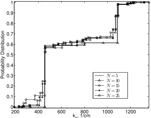
Yj =|r(kj;G0)|2+Ej, j= 1,2,3, . . . , N, (2.3.1) with r(k;G) given by (2.1.3). The simulated data is then generated by simulating

(38)

In the above equation, G0 is chosen as the cumulative distribution function of a truncated normal distribution with its corresponding probability density functionp0 given by

p0(k0) =

β σ√2πexp

−(k0−µ) 2 2σ2

, k0∈[k0,¯k0],

where µ= 700, σ= 50, k₀ = 400, ¯k0 = 1090, and β is the normalizing constant

β−1 =

Z ¯k0 k0

1

σ√2π exp

−(k0−µ) 2 2σ2

dk0.

The j are realizations ofEj, which are assumed to be normally distributed with zero mean and standard deviationσ0= 0.002. For all the simulations below,N is chosen as 70, the measurement wavenumber points are kj = 400 + 10(j−1), j = 1,2, . . . ,70, and the values for the rest of model parameters are chosen as

τ = 0.03, εs = 2.7, ε∞= 2.5.

SinceG0 is chosen as an absolutely continuous function, we will use the linear spline approxima-tion method in the simulaapproxima-tions demonstrated below.

In the presentation below, we first use the Akaike Information Criterion to determine the optimal value ofM, where the probability measure is obtained by the linear spline approximation method. We then compare the confidence band obtained using the asymptotic normality results with the one obtained with the Monte Carlo simulations.

2.3.1 Optimal Value of M

As we stated earlier in this section, we use the Akaike Information Criterion (AIC), one of the most widely used model selection criteria, to determine the optimal value for M. The AIC was developed by Akaike (in 1973), and it is based on Kullback-Leibler information (a well-known measure of “distance” between two probability density functions) and maximum likelihood estimation. There are several advantages in using the AIC. For example, it can be used to compare both nested models and non-nested models, and it can also be used to compare multiple models at a time. For the least squares case, it can be found (e.g., see [46, Section 2.2], [33, Section 4.3.1]) that if the measurement errors are i.i.d. normally distributed, then the AIC is given by

AIC =Nlog

RSS

N