A DIRECT ASSESSMENT OF THE ROLE OF GENETIC
DRIFT IN DETERMINING ALLELE FREQUENCY
VARIATION IN POPULATIONS OF EUPHYDRYAS
EDITHA
LAURENCE D. MUELLER,* BRUCE A. WILCOX,** PAUL R. EHRLICH,** DAVID G. HECKELt AND DENNIS D. MURPHY**
*Department of Zoology and Program in Genetics, Washington State University, Pullman, Washington 99164; **Department of Biological Sciences, Stanford University,
Clemson, South Carolina 29631
Manuscript received March 9 , 1984 Revised copy accepted March 2, 1985
Stanford, Calqornia 94305; Department .f Biologtcal Sciences, Clemson University,
ABSTRACT
Estimates of allele frequencies at six polymorphic loci were collected over eight generations in two populations of Euphydryas editha. We have estimated, in addition, the effective population size for each generation for both popula- tions with results from mark-recapture and other field data. T h e variation in allele frequencies generated by random genetic drift was then studied using computer simulations and o u r direct estimates of effective population size. Substantial differences between observed values and computer-generated ex- pected values assuming drift alone were found for three.loci (Got,
Hk,
Pgi) in one population. These observations are consistent with natural selection in a variable environment.OR nearly
20 yr empirical population genetics has grappled with the prob-
F
lem posed by the large amounts of genetic variation found in natural
populations. Evidence supporting the neutral theory of molecular evolution
has usually come from comparisons of data to certain stationary properties of
neutral models. Properties of natural populations such as the expected heter-
ozygosity, variance in heterozygosity and frequency spectrum are seen to be
in reasonable accord with predictions from the neutral model
(FUERST, CHAK-
RABORTYand
NEI
1977;
CHAKRABORTY,
FUERST
and
NEI
1980). Those work-
ers who feel that most polymorphisms are maintained by natural selection have
taken a different approach to the problem and have produced a number of
independent investigations of particular polymorphic loci in several organisms
(MCDONALD
and
AYALA
1978;
PLACE
and
POWERS
1979;
BURTON
and
FELD-
MAN
1983;
WATT,
1983;
WATT, CASSIN
and
SWAN
1983). Such studies aim to
establish the biochemical and physiological differences between electrophoretic
variants and then to relate these to pertinent ecological data to develop a
coherent picture of the forces maintaining the particular polymorphism.
Recently, many of the statistical tests of the neutral theory have been ques-
tioned.
ROTHMAN
and
TEMPLETON
( 1
980) show that
EWENS’
(1972) sampling
496
L.D.
MUELLER ET AL.theory and tests based on it (WATTERSON
1977) rely on a special assumption
about the distribution of the number of copies of neutral alleles. When this
assumption is relaxed the resulting neutral models can yield frequency spectra
and homozygosities similar to those expected from heterosis. GILLESPIE
(1
979)
has shown that the infinite allele model and his model of selection in a random
environment have the same stationary distribution. Therefore, the agreement
between empirical observations and the infinite allele model noted by FUERST,
CHAKRABORTY
and NEI (1977) can be used with equal strength to support
Gillespie’s model of natural selection. Another problem with these tests is the
assumption that the study population has reached its stationary distribution. A
population undergoing a variety of drift processes approaches its stationary
distribution at a rate governed by the second largest eigenvalue which equals
1
-
const/2N, where N is the effective population size. If N is even moderately
large this rate can be extremely slow. PERLOW
(1979) has shown that the
elegant test of the infinite allele model devised by WATTERSON
(1977)
IS.
sen-
sitive to the stationary assumption.
Several tests of the neutral theory have been devised which use observations
of allele frequencies over several generations. T h e first such test was described
by LEWONTIN
and
KRAKAUER
(1973). Their test was based on calculating stand-
ardized variances of allele frequency changes over one or several generations
in the same population.
In their initial work, however, Lewontin and Krakauer
did not properly account for the sampling process in allele frequency estima-
tion; corrections for this have been noted since by PAMILO
and VARVIO-AHO
(1980), NEI and
TAJIMA
(1981) and POLLAK
(1983). Yet, to use this method
as a test of neutrality, the sampling distribution of the standa5dizep variance,
P,
must be known. NEI and
TAJIMA
(1981) have shown that
nF/E(F), where
nis the number of independent alleles (or loci) used to estimate
F,
has a
x 2
distribution with
n
degrees of freedom. However, we do not generally know
E@)
and it is not clear that, if this quantity is replaced with a small sample
estimate, the
x 2
distribution will be preserved. Furthermore, even when
E @ )
is known the
x 2
approximation becomes worse if
@
is based on observations
separated by several generations. Finally, it is not at all clear what
will happen
to the distribution of
&/E(@)
if more than one generation has passed and the
effective population size does not remain constant over time.
Other tests of neutrality that utilize temporal data have been described by
FISHER
and FORD
(1 947), SCHAFFER,
YARDLEY
and ANDERSON
(1977) and WAT-
TERSON
(1 982). However, both of these tests require precise knowledge of the
effective population size. Unfortunately, this is seldom known for natural pop-
ulations. At best an estimate of total population size may be available from
mark-recapture techniques.
497
advantages of computer intensive statistics have been discussed by
DIACONIS
and
EFRON (1983).
We also investigate the ability of o u r test procedure
to
detect modes
of
natural selection that increase the variation in allele frequencies. We find that
our methods are able to detect selection that increases allele frequency varia-
tion, such as selection in a random environment.
MATERIALS AND METHODS
Genetic and ecological data have been collected for the univoltine checkerspot butterfly Euphy- dryas editha, an endemic of serpentine grasslands in the San Francisco Bay Area. Two populations, known from areas H and C, were studied at Jasper Ridge Biological Preserve on the Stanford University campus, California, from 1973 and 1980 (EHRLICH et al. 1975; EHRLICH and MURPHY
1981). Adults fly and oviposit from approximately mid-March through late April. Thus, the life cycle is composed of truly discrete nonoverlapping generations.
Genetic data: Electrophoretic data were collected each year for six polymorphic loci: glutamate- oxaloacetate transaminase (Got), hexokinase
(HK),
@-hydroxybutyric acid dehydrogenase (Hbdh),phosphoglucose-isomerase (Pgi), phosphoglucomutase (Pgm) and superoxide dismutase (Sod). Details of the electrophoretic methods are given by MCKECHNIE, EHRLICH and WHITE (1975).
Estimating adult numbers: Population size data were also collected each year using the mark- recapture methods of BRUSSARD, EHRLICH and SINGER (1974) and EHRLICH and DAVID” (1 960).
In brief, each year’s study of a population consisted of several separate census visits to the site during which adult individuals were captured, individually marked if not already marked and released. These data were used to estimate the size of the population according to the Jolly-Seber model (SEBER 1973, chapter 5, correction for bias not employed). T w o features of the Euphydryas census data make the Jolly-Seber method particularly appropriate here: (1) The population is open, i.e., the adult population size is constantly changing in time as newly eclosed adults augment it and dying or emigrating adults diminish it. (2) Both weather (flight) conditions and sampling effort vary from time to time, and therefore, capture probabilities are potentially different for each separate census visit. The Jolly-Seber model is a widely used method that takes account of both of these features of the population. It provides estimates of N,, the population size at census visit i, for all census visits except the first one. It also allows estimation of E,, the number of new aduks entering the population between samples
i
and i+
1. For our estimate of total population size B for a site at a given year, we summed all of the B, corresponding to that year and site. The variance of the estimate of B was obtained from Jolly’s (see SEBER 1973, chapter 5) formulas for the variances and covariances of the B, and the general formula for the variance of a sum of random variables.I t became necessary to employ a slight modification of the Jolly-Seber method when m,, the number of previously marked butterflies caught in the ith sample, equaled zero. Under these conditions, the estimate of N , becomes undefined. Rather than to arbitrarily employ some bias- correcting alteration in the formula for N,, we chose to pool the animals of sample i with those of sample i - 1 under these conditions. Also, the Jolly-Seber method does not give an estimate of
N I (= Bo), the number of animals that joined the population before the first census visit and survived to that time. Usually, we have not attempted to estimate N I ; instead, we ignore it and confine our problem to estimating the total number of individuals that joined the population during the time spanned by the census visits. Because there are always some individuals present at the time of the first visit, we are thereby underestimating the total size of the population, but this is only a slight underestimation because the first census is placed early in the flight season and most of the butterflies eclose during the time spanned by the census. On two occasions URH 1974, 1978) our data pooling resulted in a large number of individuals being present at the first census. In these two cases we estimated the total number present on day 1 using the number captured and the probability of capture for the second census date. This number was added to the standard estimate of total population described previously.
498
I,. D. MUELLER E T AL.separate estimates of the number of males B , and females B, are usually available. In some years the sex ratio was quite biased with females making up only IO-20% of the population. Unfortu- nately, the variance of the estimates of the separate male and female numbers is much larger than the estimate of total population size with males and females pooled. This is important in the decision to use separate B, and B,, o r just pooled B assuming a 1:l sex ratio, to estimate Ne. Thus, even though we expect an estimate of Ne that utilizes the separate sexes to be less biased, it is liable to have much larger variancq This, of course, will make it more difficult to detect deviations from the drift model. As a consequence we have examined four estimators N , of the effective population size. In APPENDIX 1 we derive an inbreeding effective population size that takes into account unequal sex ratio, variance in female reproductive success and changing population size. Four versions of this effective population size are considered which make various assumptions about the sex ratio and population growth. As noted by EWENS (1982), the inbreeding effective size will not necessarily be the same as the variance or eigenvalue effective population size; how- ever, its derivation appears to be much simpler in the present setting. T h e estimator with the smallest mean squared error was used as Ne in the computer simulations. This procedure does introduce a bias in our results which we consider in the discussion.
In a few years females were so rare that not enough were recaptured to allow a direct estimate from the Jolly-Seber procedure. In these years we estimated the frequency of females in the population, c, from their frequency in the captured pool of animals. Since males are almost twice
as likely as females t o be captured (EHRLICH, LAUNER and MURPHY 1984), c is probably biased downward. T h e effect of this will be estimates of Ne that are too small. We will discuss the effect of this bias on o u r test statistics later. T h e total number of females
N,
was then estimated as B . c ,and the total number of males
N,
as B . ( l-
c). T h e variance of these estimates were obtained via the delta method (BISHOP, FIENBERC and HOLLAND 1975; pp. 486-488).Variance in offSpring number: Another factor that has a significant effect on the effective popu- lation size is the variance in offspring number and survivorship which is substantial between females. This variability can be partitioned into a t least three components. First, there is variability in the number of eggs laid per egg mass and the number of egg masses. Females may lay between
40 and 200 eggs per egg mass, and in the laboratory they may lay up to seven egg masses or more, although four is perhaps more typical in the field. Second, there a r e marked differences in survival of egg masses laid in wet and dry environments. E. editha usually lays eggs on green
Plantago erecta and Orthocarpus densajlorus. However, these plants may undergo rapid senescence, and the larvae may hatch into a dry environment in which mortality is virtually 100% (SINGER
and EHRLICH 1979). Third, there is variability in larval survival even within wet environments. Assuming that these three factors act independently of each other, we can derive formulas for the mean and the variance of female offspring number (see APPENDIX 2 for details). Let the random variable W, be the number of surviving offspring from a female’s ith egg mass. T h e mean number of surviving offspring from egg mass i is E(Wi), and the formula for it is found to be
E(WJ = X(1 - 6 ) u , =
w,,
where U% is the mean number of eggs in egg mass i, 6 is the probability that the egg mass hatches into a dry environment and X is the individual probability of survival from larva to adult in a wet environment. T h e variance in number of surviving offspring from egg mass i is Var(W,), which is
where U:, is the variance of the number of eggs in egg mass i. If it is assumed that the separate egg masses of a female are independent, the total variance in female fecundity Var(F) is just the sum of the Var(W,) over egg masses.
T h e actual calculations of Var(F) make several assumptions. Although females may lay up to seven egg masses, o u r experience indicates that four egg masses may be more typical in the field. T h e mean number of eggs per mass and the variance are estimated from the work of MURPHY, LAUNER and EHRLICH (1983) which looked at female fecundity as a function of diet. We assume the diet of sugar water and 0.004 M amino acids to be most similar to the diets available on Jasper Ridge. We also assume that the probability of hatching into a dry environment (6) is 0.71. SINGER
A
Infinite number
sample of N1
2 PO
allele frequency random union of zygotes in
in gamete pool
-
Hardy-Weinberg zygotes whereproportion A
NI”N(N1 , O N 1 )
499
A
A A
.L
....
ib
P*NS1 adults sampled without replacement
allele A N, adults frequencies with
L+
allele frequency p1-w
....
in the gamete pool first generation
P1
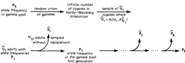
FIGURE 1.-The life cycle used in the computer simulation that incorporates random genetic drift and sampling of allele frequencies.
toward the higher end of this range (actually the value observed 1 wk into the 1971 flying season). The possible biases this choice might introduce is discussed later. Finally, X is chosen such that each female at time t had, on average, 2Nl+i/N, offspring in the next generation. For models I and 111 (see APPENDIX 1) it is assumed that N,+I = N,. Models I1 and IV allow for population increase and decrease and, therefore, use the actual estimates of total population size N , and N l C l .
Carrying o u t the calculations produces an estimate for the variance in female fecundity of 5.49 when N1+, = N,.
Comparison with indirect estimates of effective population size: Recently, there have been several proposals to estimate effective population size indirectly from observations of allele frequency variation over time (NEI and TAJIMA 1981; POLLAK 1983). These methods assume that variation in allele frequencies over time is due solely to genetic drift and sampling for estimation purposes. Since we hope to use our estimates of effective population size to determine whether drift alone can account for the observed variation, it would seem inappropriate to use these methods to estimate effective population size. However, these methods consistently produce estimates of ef- fective population size that are about one order of magnitude smaller than estimates obtained by several other methods (POLLAK 1983; BECON, KRIMBAS and LOUKAS 1980). The same is true for our data. As we show in the next section Pollak’s method of estimating effective population size is sensitive to the presence of variable natural selection. Thus, we feel justified in disregarding these estimates.
Computer simulations of Euphydryas population genetics: We now ouline the life cycle used.in our computer simulations (Figure 1). The dynamics of a single locus with
k
alleles will be modeled. The frequency of the j t h allele at time t is P,,. The vector of all allele frequen-es at time t is represented byP,
= (PI,, , P i - l , f ) T . At generation t drift occurs by sampling N, zygotes from an infinite zygote pool. S e we only have estimates of the effective population size,G1
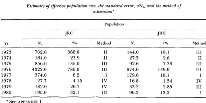
is a random variable chose? from a normal distribution with mean N, and variance U;, which are given in Table 1. After the N1 adults have produced the gamete pool for the next generation, N,, adults are sampled without replacement to estimate the allele frequency vectorP,.
This estimate is denotedP,.
The N,, are known exactly and correspond to the actual sample sizes used to estimate allele frequencies in the various Euph yas populations. After eight generations of drift the covariance matrix of the observationsPI,
,Ps
was calculated. At this point, one iteration is complete.A total of 1000 iterations were performed. Thus, there were 1000 covariance matrices for the drift-only process from which we made statistical inferences. All of the loci used in this survey were polymorphic, and there was no indication that any allele became fixed or lost in the eight generations of observations. Thus, if during the course of the
computer
simulation an allele was lost or fixed, that particular sequence of allele frequency vectors was ignored. Because of the small number of generations considered, mutation and migration $an be ignored. The initial allele frequencies were set to the observed values in 1973.500
L. D. MUELLER E T AL.TABLE 1
Estimates of effective population size, the standard error,
UN.,
and the method of estimation'Population
Yr
n;,
UN, Method N . U& Method1973 1974 1975 1976 1977 1978 1979 1980 762.0 164.0 856.0 4022.0 374.0 27.7 182.0 195.0 366.0 23.9 135.0 786.0 6.2 4.15 20.7 32.1 I1 11 111
I l l
I IV IV 111 144.0 27.5 92.6 974.0 179.0 16.8 33.2 90.2 18.1 2.6 7.39 149.0 18.1 1.54 2.85 13.2 111 I1 I11 I11 I IV 111 I
a See APPENDIX 1 .
than two alleles we have calculated the covariance matrix of
P.
Let the covariance matrix resulting from the i t h iteration be Si. I f we perform a total of m iterations, then we estimate .!?(Si) asFor each sample covariance matrix we calculate the following statistic, X, = ( t
-
l)IInIZoI-InIS,I+ trS,Z;'-
( k-
1 ) I ,where t is the number-of generations (eight in our case) and k is the number of alleles at the particular locus. If the
P,
have a multivariate normal distribution then X, willP,
distributed asx2
k(k
-
1)/2 (MORRISON 1976, p. 248). T h e r e is no reason to assume that theP,
has a multivariate normal distribution, so the purpose of the computer simulation is to describe empirically the distribution of the X, under the drift-only hypothesis.RESULTS
T h e final estimates of effective population size with their standard errors
are given in Table
1 for both populations JRC and JRH. In Table
2
we present
the yearly allele frequencies and sample sizes for both JRC and
JRH.
Only the
alleles used to calculate the covariance matrix are given in Table
2.
Following the scheme outlined in Figure
1 w e have calculated the expected
covariance matrices for each locus assuming the effective population sizes listed
in Table
1. These expected covariance matrices and their observed values are
given in Table 3. For loci with just two alleles we have computed the expected
variance and the distribution of this variance. T h e cumulative distribution of
this variance is given by
4(x)
=prob. (the observed value of the variance
is
SX).Clearly,
if this probability is
very small, or very large, then our observa-
tion represents an unlikely event and we might question the underlying as-
sumptions. In Table
3 we have listed the value of
4(x)
for each two-allele locus
( H k ,
Got, Sod), where
x=
the observed variance
of the most common allele.
For loci with more than two alleles our test statistic was
Xi.
T h e value of
hi
501
the expected value. In fact, when
Si
=
20,Xi
=
0. From the computer simu-
lations we have estimated the expected covariance matrix and the distribution
of
Xi.
For loci with more than two alleles
(Hbdh, Pgz, Pgm) we have a cumu-
lative distribution,
4(x)
=
prob. (observed value of
Xi
is
I x ) .
Thus, only when
4(x)
is very large (close to 1)
will we question our underlying hypothesis. These
values of
4(x)
are also given in Table
3.
From Table
3 we see that there are three cases, out of 12, that show extreme
test statistics,
e.g.,
$(x)>
0.95. These loci are Got,
Hk
and
Pgz
in population
JRC. Each of these loci shows more variation than expected from drift alone.
We expect that 12 independent applications of this test would produce
0.6
significant results by chance alone. In addition such chance deviations would
be as likely to show less variation as more variation. Clearly, overdominance
cannot account for these results. However, if selection varies over time, then
we might expect more variation than drift alone would produce. T o study this
possibility we have examined the stochastic-additive-scale constant-fitness-func-
tion (SAS-CFF) model of
GILLESPIE
(1978). [We will review only a few impor-
tant features of the symmetric SAS-CFF model here;
GILLFSPIE
(1978) should
be consulted for additional details.] We assume that the activity of the enzyme
products coded for
by
genotype
AiAi
can be described by a random variable
x i .
Heterozygotes are assumed to have an activity exactly intermediate between
the two homozygotes; thus, the net activity of enzyme products of genotype
AiAj
is
( x i
+
xj)/2.
We assume further that
E ( x i )
=
1, Var(xi)
=
a'and
cov(xixj)
=
pg'.Finally, we assume there is some concave function that ade-
quately describes the relationship between fitness and enzyme activity. For this
study we have utilized the function (1
+
.)xi/(.+
xi),where
a
is a constant.
T o conduct the appropriate computer simulations with the SAS-CFF model
we must specify values for
rs2,
pand
a.
Once done, the previous simulation was carried out as before, but viability
selection is assumed to act after drift and prior to the sampling of allele
frequencies. After each round of eight generations of drift and selection, we
compute the covariance matrix and compare it to the critical value which yields
a
5%
type
I error rate. After approximately 1000 replications of this process,
the frequency with which the drift plus selection process exceeds the critical
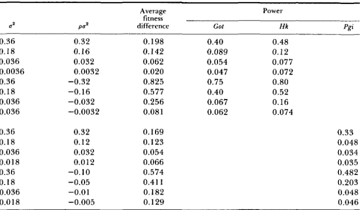
value is computed. This is simply the power of the statistical procedure. T h e
strength of selection in these computer simulations is summarized
by
comput-
ing the mean difference between the least and most fit genotype each gener-
ation. These results are given in Table
4.
503
o*
m o o a
0 9 ?
m m - 0 0
a
0 9 1
- m
- 0 0
9 9
em P -
b o o
*
o ! 9$ 2
m o o2
m -
0 0 0 0 097
0,
0 0 0
0 9 1
z o o
m - 0 0 0
W
0 9 1
0 -
= ? ?
U &-
5
g :
m o o
m
W O
a 0 0
0
P - ”
c n o
P - ” z o o
C O * m o o
9
0 9 1
at-
m o o ? ?
m
- *
- 0 0
m
0 9 1
* m 0.100 0 099
F ;
0.100 102
-7 m m o a o! m0 . 1 0
a 09
a
- 0 09 e P- - 0 m o! m a 0 m o!
-
*
I - 0 o!0,
0.1
Q!
2 0
m
m o
9
m 0 U%
z
QI n 0
CO o! m 0 0 a o!
*
moo In o!*
0 0 m9
P- a 0 00 o! am o
9
m
*
0 . 1 0 m
o!
m
5 04 L. D. MUELLER E T A L .
h
-
X -8(J1
a
cl
i:
mcn
M a r - 0 . 4
- 0 0 -
0 0 0 0
0 0 0 0
9 9 9 9
w- w m
m- I. cn
-
-
0 0 0 0 0 0 08 8
8 8
m W
r 3 c - W b O o c -
0 - m o m m
0 0 0 0 0 0
0 0 0 0 0 0 9 9 9 9 9 9
I I I I
d
.
- m m m m-,- ( 0 3 m m m 3
N"CO - m O b - - e m
3 0 0 0 0 0 0 0 0 0 0 0
3 0 0 0
I I
? 9 0 9
8 8 8 8 8 8 8 8
I
m m L
m c - e m -
0 . 4 m o o c . 1
0 0 0 0 0 0 0 0 0 0
o o o o c
I
'
c - mI
3 d c-" m I-
505
TABLE 4
The probability of detecting selection (power) with type I error set at 5%
Average Power
fitness
a2 P U P difference Got Hk Pgi
0.36 0.18 0.036 0.0036 0.36 0.18 0.036 0.036 0.32 0.16 0.032 0.0032 -0.32 -0.16 -0.032 -0.0032 0.198 0.142 0.062 0.020 0.825 0.577 0.256 0.081 0.40 0.089 0.054 0.047 0.75 0.40 0.067 0.062 0.48 0.12 0.077 0.072 0.80 0.52 0.16 0.074 0.36 0.18 0.036 0.018 0.36 0.18 0.036 0.0 18 0.32 0.12 0.032 0.0 12 -0.10 -0.05 -0.01 -0.005 0.169 0.123 0.054 0.066 0.574 0.41 1
0.182 0.129 0.33 0.048 0.034 0.035 0.482 0.203 0.048 0.046
The parameters U’ and pa’ from the SAS-CFF model are listed: CY was four in each case. The
fitness difference is the average difference between the most and least fit genotypes.
TABLE 5
Pollak’s estimates of effective population size, Ne, with symmetric variable
selection (SAS-CFF)
Average fitness
2
diffrence N . Var@”)0.36 0.198 -64 4.6 X lo6
0.18 0.142 23 3.4 x 10⁷
0.036 0.062 168 1.2 x 10⁷
0.0036 0.020 190 8.6 X lo6
N o selection 0 206 3.8 X lo6
_ _ _ _ _ ~ ~
The average fitness difference between the two homozygotes is given along with the variance of the SAS-CFF model. Other model parameters are p = 0.8, N e = 200, N , = 200, (Y = 4 and Po = 0.5.
DISCUSSION
We regard the estimates of effective population size in Table
1 as the best
estimates. These values incorporate differences in sex ratios every generation,
the variance in female reproductive success and differences in population
growth. Three “extreme” covariance matrices are found in Table
S-Got,
HK
and
Pgi
in the JRC population. T h e observed covariance matrices for Got,
HK
and
Pgi both show more variation than expected from drift and both have
506
L. D. MUELLER E T A L .three tests in this region
($(x)>
0.95) can be interpreted as an excess and,
therefore, an indication of substantial deviations from some underlying as-
sumption.
As
shown in Table 4,
if the assumption of neutrality is removed
and selection
is
allowed to vary over time, large covariance matrices can be
detected with some reliability. However, even with variable selection, the
power of the tests is low unless the magnitude of selection is quite strong. We
should note here that, even if our inferences from these statistical tests are
entirely correct,
i.e.,
variable selection has been responsible for the increased
variation in allele frequencies, we cannot differentiate between selection on
the
Got,
Hk
and
Pgz
loci and selection on other genes linked to them. Only
detailed studies of specific enzyme polymorphisms, such as those of
WATT
(1977, 1983) on
Pgi
in Colias butterflies, can directly address this latter issue.
His demonstration of a “trade off” between the heat stability and kinetic effi-
ciency of different
Pgz
genotypes suggests that variable selection may be acting
directly on this polymorphism in natural populations.
It is of some interest to compare these results to those obtained in the first
analysis of temporal data by
FISHER
and
FORD
(1947). They observed variation
in the frequency of the
medionigra
allele over a 6-yr period and obtained
estimates of the total number of
Panaxia dominula
moths in a natural popu-
lation. They did not adjust the effective population size for ecological factors,
considered in the present work; rather, they assumed that the population was
no larger than their smallest observation of 1000 moths in 1943.. Application
of their statistical test indicated that allele frequencies showed much more
variation over the 6-yr period than would be expected from drift and sampling
alone.
Clearly, the results in Table
3
are dependent on accurate estimates of the
effective population size. The weakest link in obtaining the final estimate of
effective population size was the estimate of variance in female reproductive
success. The final estimates of effective population size may be too high
if
( 1 )
the probability of eggs hatching in a dry environment were considerably
higher,
(2)
there are other significant sources of death that affect whole egg
masses,
(3)
the average female has fewer than four egg masses per season, (4)
there is large variance in male reproductive success, or
( 5 )
the sex ratio were
highly skewed in the years we assumed
it
was 1:l.
ences in natural population (COBBS
1977;
OSTERGAARD
and CHRISTIANSEN
1981),
this remains an important area for future research. T o assess the pos-
sible magnitude of condition
5
we
have recomputed the JRC effective popu-
lation sizes in Table
1
taking into account the sex ratios for every year
( i . e . ,
using method
IV).
T h e harmonic mean of these new values is
133.
T h e har-
monic mean of the original JRC population sizes is
137.
Therefore, condition
5
is unlikely to have had a serious effect
on
our final test statistics.
Our final estimates of
Ne may be too small if
(1)
the probability of eggs
hatching in a dry environment is closer to
0.2
rather than
0.7,
(2)
females lay
five or more egg masses on average, or
(3)
differential capture rates of males
and females lead to an underestimate of
c.
We have already commented on conditions
1
and
2.
Condition
3
could have
substantial effects on
N e .
For instance, if the frequency of females in JRC
during
1978
were
0.5 instead of
0.34,
the harmonic mean of all population
sizes in JRC would increase from
137
to
170.
We note that, if we have under-
estimated
N e ,
then the expected variance in allele frequencies due to drift
should be even smaller than the predicted values given in Table
3.
Thus,
Got,
Hli
and Pgi
would still show more variation than expected. We stress that to
obtain direct estimates of effective population size for natural populations
sources of mortality that affect whole families should be closely examined.
A
qualitative conclusion from this work which is in accord with others
(SCHAFFER,
YARDLEY
and ANDERSON
1977;
WATTERSON
1982)
is that selection
has to be quite strong before patterns
of
allele frequency variation differ
substantially from the neutral expectations. Other aspects of genetic differen-
tiation of
E.
editha
have been used to discount genetic drift. EHRLICH
and
WHITE
(1980)
have noted that Colorado populations of
E. editha
differ greatly
from West Coast populations at the
Pgm
locus but are very similar at seven
other loci. In the absence of significant migration they argue the lack of
differentiation at most loci except
Pgm
must be due to some form of stabilizing
selection or,
if
the populations only recently split,
Pgm
should not be
so
dras-
tically different.
NEI
and
TATENO
(1975)
have shown that in some circumstances drift alone
can produce patterns of differentiation in which identities
( I l )
at some loci are
high and at others low. Their simulation results, however, show approximately
half of the loci in each category after
500
generations, with a trend toward
increasing numbers of differentiated loci with generation time. Ehrlich and
White’s results, however, show a high to low identity ratio of
7:l
(binomial
P
=
0.03
if
4:4
expected). T h e approximate number of generations since the
populations in their study were united is
7000,
and the
Ne
was probably in the
50-500 range. Furthermore, all of the loci studied by Ehrlich and White are
polymorphic in the vast majority of
E .
editha
populations (MCKECHNIE,
EHR-
LICH
and WHITE
1975),
and it is reasonable to assume that all eight loci were
polymorphic when the populations separated. In contrast, Nei and Tateno
started their simulation with about 60% of their loci monomorphic. Thus, one
would expect fewer similar loci than found in the Ehrlich-White data, but the
opposite is the case.
508
L. D. MUELLER E T A L .derive our final test statistics. T h e hope is that the final test will be more
robust than previously described tests. T h e “cost” of making fewer assumptions
is
the need empirically to determine the distribution of test statistics via com-
puter simulations. We point out that this procedure results in major differences
in our final test criteria. For instance, the value of
Xi
for population
JRH
and
locus
Pgi
was 10.9. If we had assumed that the allele frequency vectors were
samples from a trivariate normal distribution, then our test statistic would have
a
x 2
distribution with
6
d.f. Consequently, for this value
of
Xi,
$(x) E0.91,
which indicates a nearly significant result. From our empirical distribution of
A,
w e
observe that the true value of
+(x)is
0.35.
Note that the computer
simulations provide our expected value of the covariance matrix in addition
to determining the distribution of
A,.
T o derive this quantity analytically would
be difficult at best without a number of additional simplifying assumptions.
This work was supported by National Science Foundation grant DEB 82-06961 to P. R. EHR-
LICH, National Institutes of Health grant GM 28016 to M. W. FELDMAN, National Institutes of
Health National Service Award GM 07310 from the National Institute of General Medical Sciences t o L. D. MUELLER and a grant from the Koret Foundation of San Francisco. We thank MARCUS
W. FELDMAN, JEFF POWELL and two anonymous referees for comments on a draft of this manu- script.
LITERATURE CITED
BEGON, M., C . B. KRIMRAS and M. LOUKAS, 1980 T h e genetics of Drosophila subobscura. XV.
Effective size of a natural population estimated by three independent methods. Heredity 45: 335-350.
BISHOP, Y : M., S. E. FIENRERC a n d P. W. HOLLAND, 1975 Discrete multivariate analysis: theory and practice. M I T Press, Cambridge, Massachusetts.
BRUSSARD, P., P. R. EHRLICH a n d M. C. SINGER, 1974 Adult movements and population structure in Euphydryas editha. Evolution 28: 408-415.
Physiological effects of an allozyme polymorphism: glutamate-pyruvate transaminase and response to hyperosmotic stress in the copepod Tzgriopus calfornicus. Biochem. Genet. 21: 239-251.
CHAKRABORTY, R., P . A. FUERST and M . NEI, 1980 Statistical studies on protein polymorphism in natural populations. 111. Distribution of allele frequencies and the number of alleles per locus. Genetics 94: 1039-1063.
Multiple insemination and male sexual selection in natural populations of Dro-
Measurement of gene frequency drift in small populations. Computer-intensive methods in statistics. Sci. Am. 248: 116-
Techniques for capture-recapture studies of Lepidop- Can sex ratio be defined or determined? BURTON, R. S. and M. W. FELDMAN, 1983
CORRS, G., 1977
sophila pseudoobscura. Am. Nat. 111: 641-656. CROW, J. F. and N. E. MORTON, 1955
DIACONIS, P. and B. EFRON, 1983
EHRLICH, P. R. and S. E. DAVIDSON, 1960
EHRLICH, P. R., A. E. LAUNER and D. D. MURPHY, 1984 Evolution 9: 202-2 14.
130.
tera populations. J. Lepid. Soc. 14: 227-229.
T h e case of a population of checkerspot butterflies. Am. Nat. 1 2 4 527-539. (Euphydryas). Biol. Zentralbl. 100: 6 13-629.
and the biospecies. Am. Nat. 115: 328-341.
EHRLICH, P. R . and D. D. MURPHY, 1981 T h e population biology of checkerspot butterflies
509
EHRLICH, P.
R.,
R. R. WHITE, M. C. SINGER, S. W. MCKECHNIE and L. E. GILBERT,EWENS, W.
J.,
1972 The sampling theory of selectively neutral alleles. Theor. Pop. Biol. 3: 87-EWENS, W.
J.,
1979 Mathematical Population Genetics. Springer-Verlag, Berlin.EWENS, W.
J.,
1982 On the concept of effective population size. Theor. Pop. Biol. 21: 373-378.FISHER, R. A. and E. B. FORD, 1947 The spread of a gene in natural conditions in a colony of FUERST, P. A., R. CHAKRABORTY and M. NEI, 1977 Statistical studies on protein polymorphism
GILLESPIE, J. H., 1978 A general model to account for enzyme variation in natural populations.
GILLESPIE, J. H., 1979 Molecular evolution and polymorphism in a random environment. Ge-
LEWONTIN,
R.
C. and J. KRAKAUER, 1973 Distribution of gene frequency as a test of the theoryMCDONALD, J. F. and F. J. AYALA, 1978 Gene regulation in adaptive evolution. Can. J. Genet.
MCKECHNIE, S. W., P. R. EHRLICH and R. R. WHITE, 1975 Population genetics of Euphydryas
1975
112.
Checkerspot butterflies: a historical perspective. Science 188: 22 1-228.
the moth Panaxia dominula L. Heredity 1: 143-174.
in natural populations. I. Distribution of single locus heterozygosity. Genetics 86: 455-483.
V. The SAS-CFF model. Theor. Pop. Biol. 14: 1-45.
netics 93: 737-754.
of selective neutrality of polymorphisms. Genetics 74: 175-195.
Cytol. 20: 159-175.
butterflies. 1. Genetic variation and the neutrality hypothesis. Genetics 81: 57 1-594.
Multiuariate Statistical Methods, Ed. 2. McGraw Hill, New York. MORRISON, D. F., 1976
MURPHY, D. D., A. E. LAUNER and P. R. EHRLICH, 1983 The role of adult feeding in egg production and population dynamics of the checkerspot butterfly Euphydryas editha. Oecologia
Genetic drift and estimation of effective ?opulation size. Genetics
lnterlocus variation of genetic distance and the neutral mutation theory. Proc. Natl. Acad. Sci. USA 72: 2758-2760.
Selection component analysis of natural poly- morphisms using population samples including mother-offspring combinations, 11. Theor. Pop. Biol. 19: 378-419.
Letter to the editor on the estimation of population
The transition density for multiple neutral alleles. Theor. Pop. Biol. 16: 223-
Genetic variation and relative catalytic efficiencies: lactate dehydrogenase B allozyme of Fundulus heteroclitus. Proc. Natl. Acad. Sci. USA 76: 2354- 2358.
A new method for estimating the effective population size from allele frequency A class of models of selectively neutral alleles.
Drift or selection: a statistical test of
5 6 257-263.
NEI, M. and F. TAJIMA, 1981
NEI, M. and Y. TATENO, 1975
~ S T E R G A A R D , H. and F. B. CHRISTIANSEN, 1981
98: 625-640.
PAMILO, P. and S. L. VARVIO-AHO, 1980
size from allele frequency changes. Genetics 95: 1055-1057.
232.
PERLOW, J., 1979
PLACE, A. R. and D. A. POWERS, 1979
POLLAK, E., 1983
changes. Genetics 104: 53 1-548.
ROTHMAN, E. D. and A. R. TEMPLETON, 1980
Theor. Pop. Biol. 18: 135-150.
gene frequency variation over generations. Genetics 87: 37 1-379.
don.
SCHAFFER, H. E., D. YARDLEY and W. W. ANDERSON, 1977
510
L. D. MUELLER E T AL.SINGER, M . C. and P. R. EHRLICH, 1979 Population dynamics of the checkerspot butterfly Eu-
phydryas editha. Fortschr. Zool. 25: 53-60.
Adaptation at specific loci. I. Natural selection on phosphoglucose isomerase of Colias butterflies: biochemical and population aspects. Genetics 87: 177-1 94.
Adaptation a t specific loci. 11. Demographic and biochemical elements in the maintenance of the colias PGI polymorphism. Genetics 103: 691 -724.
Adaptation at specific loci. 111. Field behavior and survivorship differences among Colias PGI genotypes are predictable from in vitro bio- chemistry. Genetics 103: 725-739.
Heterosis o r neutrality? Genetics 85: 789-814.
Testing selection a t a single locus. Biometrics 38: 323-331.
WATT, W. B., 1977
WATT, W . B. 1983
WATT, W . B., R. C. CASSIN and M. S. SWAN, 1983
WATTERSON, G . A., 1977
WATTERSON, G . A., 1982
Communicating editor: J. R. POWELL
APPENDIX
1
In this appendix w e derive an inbreeding effective population size, N e , which takes into account the relevant ecological details of Euphydryas. Our derivation closely follows the methods outlined by EWENS (1979). T h e inbreeding effective population size is defined as the reciprocal of the probability ( x ) that two different alleles chosen a t random in generation t
+
1 are descended from the same individual in generation t. Let N I be the number of males andNz
the number of females in generation t. T h e total population size in generation t , N I , is clearly the sum of N I andNz.
For female i we denote the number of descendent alleles produced from each of i ' s two copies by m, and mNZ+,. For malei
we denote similar quantities asp,
andpN,+,.
Since each individual at timet
+
1 has one allele from a female and one from a male the following relationships hold,N I
NIP=
(p,
+
$'NI+,) = Nt+I,, = I
NZ
Ne6 =
1
(mi+
m N 2 + J = N,+I,,=1
where NI+] is the total number of individuals in generation t
+
1 . Following arguments similar to EWENS' (1979, p. 106) we see that?r = (Ni+l - 1)[2(2Nt+I - I)]-'
c
( p i+
t N l + i ) ( f i+
, ~ N I + , - 1 ).[z(pi
+
f i N , + i ) ] - ' [ z ( p i+
p N l + < ) - I]-'+
I f w e let V, be the variance of the m,'s and V, the variance of the pi's then,
x = [ 2 ( 2 6 N * - l)]-l[vp/j
+
V J I+
p
+
m-
21.T h u s ,
N e = 2(2INz
-
l)(Vp/j+
V,/m+
p
+
I-
2)-'.Since we have no information about the variance in male reproductive success, we assume
Vp/p = 1 , yielding
Ne = 2 ( 2 i N 2
-
l)[Vm/m+
6 ( N z / N I+
1)-
1]-'. (1A)5 1 1
Model I: Equal sex ratio, no population growth. These assumptions imply that N I = N 2 = N 1 / 2
and m = 2 ; thus,
Nei = 2(2Nt
-
1)(Vm/2+
3)-’. (2‘4)Model ZZ: Equal sex ratio, population growth. With these assumptions we have N I = N2 = N 1 / 2
and m = 2Nl+1/Nl; thus,
Neil
= 4NiNi+1(2Ni+1 - l ) ( V R N :+
8N!+1 - 2NiNi+i)-l.N ~ I I I = 2NtNiN2(2Ni
-
1)[N1N2(N2Vm-
N t )+
N:]-’.Neiv = 2NiNzNt+1(2Ni+i
-
l)[NiNz(NZV, - Nt+i)+
N : + I ( N I+
N2)I-l.(3‘4)
Model ZZZ: Unequal sex ratio, no population growth. These assumptions imply m = N t / N z ; thus,
(4‘4)
Model ZV: Unequal sex ratio, population growth. With this model 6 = N1+I/N2; thus,
(5‘4)
APPENDIX
2
Let us define some terms. Let Xi be a random variable that represents the number of eggs laid by a female in her ith egg mass. A particular realization of this random variable will be denoted
xi. We also have E(Xi) = and Var(Xi) = 0;. If d is the probability of an egg mass hatching into a dry environment, then let Y be an indicator random variable with
0 with probability 6 1 with probability 1
-
6Z, will be a Bernoulli random variable and, as before, zj will be a realization of Z,. If the larvae
survive dessication, we assume they survive to become adults with probability X. Thus, in a mass of x, eggs that have survived dessication, the number that survive to adulthood, W,, will be
z j . The fate of egg j is survival to adulthood (if z, = 1) or death (if z, = 0). Finally, we let the total number of larvae from egg mass
i
that survive to adulthood to be Wi. Clearly, we now seek an expression for E(W,) and Var(W,).In both cases we find the expected values by conditioning successively on the values of X,, Y and
2;~;
Z,. Thus,Y =
1
E(Wi) = EIEIE(E[Wilxi, yp Z z j l l l l . Solving this we get
E z,~x,, y = x , y ~ since ZZ, - B ( x , ~ x , ~ ( 1 - h)x,y),
E[x,YXJx,] = Xx,(l
-
a),
1
E[X(l
-
6)X,] = E(W,) = X ( l-
6)ux, = W,. We do the same sort of conditioning to get Var(W,). After some algebra we see thatvar(w,) = W,[1
-
x
-
W,+
~ a z , / u ,+
XU,].Since the total fecundity, F , is equal to