Pohl, Sara (2018): Track reconstruction at the first level trigger of the Belle II experiment. Dissertation, LMU München: Fakultät für Physik

(1)

Track Reconstruction at the First Level

Trigger of the Belle II Experiment

Sara Pohl

(2)

(3)

Track Reconstruction at the First Level

Trigger of the Belle II Experiment

Sara Pohl

Dissertation

der Fakultät für Physik

der Ludwig-Maximilians-Universität

München

vorgelegt von

Sara Pohl (geb. Neuhaus)

aus Starnberg

(4)

(5)

Zusammenfassung

Das Belle II Experiment ist ein Upgrade des Belle Experiments, das wesentlich zur Bestätigung der Kobayashi-Maskawa Theorie über den Ursprung derCP-Verletzung beigetragen hat. Der neue e+_e−_{Beschleuniger SuperKEKB soll eine instantane}

Lumi-nosität von 8×1035cm−2_s−1_{erreichen und damit den Weltrekord seines Vorgängers}

KEKB um einen Faktor 40 übertreffen. Belle II wird sowohl Präzisionsmessungen an B-Mesonen durchführen als auch Suchen nach seltenen Zerfällen, wie beispielsweise Lepton-Flavor verletzendeτ-Zerfälle.

Infolge der erhöhten Luminosität wird auch eine höhere Untergrundrate erwar-tet, die bereits auf der ersten Triggerstufe reduziert werden muss. Eine dominante Untergrundquelle sind Teilchen, die nicht von e+_e− _{Kollisionen stammen, sondern}

von Stößen innerhalb eines Strahls oder mit Restgasmolekülen in der Strahlröhre. Die daraus entstehenden Spuren können durch ihren Entstehungspunkt identifiziert werden, der gegenüber dem Kollisionspunkt longitudinal verschoben ist.

Im Fokus der vorliegenden Arbeit steht die 3D Rekonstruktion von Spuren in der zentralen Driftkammer des Belle II Detektors auf der ersten Triggerstufe. Die Driftkammer enthält Drähte mit unterschiedlicher Ausrichtung:Axial-Drähte sind parallel zurz-Achse gespannt, wohingegenStereo-Drähte gegen diez-Achse verdreht sind. Spuren, die von der z-Achse, aber nicht notwendigerweise vom Kollisionspunkt stammen, werden durch vier Parameter beschrieben: Den Azimuth- und Polarwin-kel, die Spurkrümmung und die longitudinale Koordinate des Entstehungspunktes („z-Vertex“). Die Spurkrümmung entsteht durch ein konstantes Magnetfeld von 1.5 T entlang der z-Achse und ist umgekehrt proportional zum Transversalimpuls des Teilchens.

Die Spurrekonstruktion im Trigger besteht aus zwei Stufen: ein Spurfindungs-algorithmus in der transversalen x-y-Ebene, gefolgt von einer 3D Rekonstruktion einzelner Spuren. Der Spurfinder bestimmt die Anzahl an Spuren sowie ihren jewei-ligen Azimuthwinkel und ihre Krümmung mittels einer Houghtransformation. Hits von Axial-Drähten entsprechen Punkten in der transversalen Ebene und werden zu Kurven in einer Hough-Ebene transformiert. Spuren werden als Kreuzungspunk-te mehrerer Kurven gefunden. Die Spurparametrisierung für diese Transformation beschreibt Halbkreise in der transversalen Ebene, die vom Ursprung nach außen laufen. Mit dieser Definition entsprechen die Koordinaten des Kreuzungspunktes in der Hough-Ebene dem Azimuthwinkel und einer vorzeichenbehafteten Krümmung, über die man den Transversalimpuls und die Ladung der Spur erhält.

(6)

die Spuren bereits durch den Spurfinder voneinander getrennt wurden, kann jede Spur separat rekonstruiert werden. Durch die Kombination von Hits der Stereo-Drähte mit der transversalen Spur können longitudinale Hit-Koordinaten bestimmt werden. Um die Ortsauflösung zu erhöhen, werden auch die Driftzeiten der Hits berücksichtigt, die proportional zum Abstand zwischen der Spur und dem Draht sind. Anstelle einer analytischen Rekonstruktion werden mehrlagige Perzeptrons (MLPs) trainiert, ein bestimmter Typ von neuronalen Netzen. MLPs können nichtlineare Funktionen aus Beispieldaten lernen und lassen sich parallelisiert mit deterministischer Laufzeit ausführen. Die Netze erhalten die Drahtkoordinaten relativ zur transversalen Spur sowie die Driftzeiten der Hits als Eingabewerte und schätzen den Polarwinkel und den z-Vertex. Für die Spuren einzelner Myonen wird eine durchschnittliche z -Vertex-Auflösung von (2.910±0.008) cm erreicht, wodurch der Großteil der Untergrundspuren unterdrückt werden kann.

Im Anschluss an die Optimierung der Houghtransformation und der neuronalen Netze wird in dieser Arbeit die Triggereffizienz ausgewählter B und τ Ereignisse

untersucht. Unterschiedliche Bedingungen des Spurtriggers werden verglichen, dar-unter ein z-Vertex-Veto und ein Veto gegen Bhabha-Streuprozesse, die im Belle II Experiment einen zweiten dominanten Untergrund darstellen. Durch die Kombination dieser Vetos können selbst Ereignisse mit nur ein oder zwei Spuren getriggert werden. Für den Lepton-Flavor verletzenden Zerfall τ_→µγ erreicht ein reiner Spurtrigger

(7)

Abstract

The Belle II experiment is an upgrade of the Belle experiment, which was instru-mental in confirming the Kobayashi-Maskawa theory for the origin ofCP violation. The upgraded e+_e− _{collider SuperKEKB is designed to achieve an instantaneous}

luminosity of 8×1035cm−2_s−1_{, which is 40 times higher than the world record set by}

its predecessor KEKB. Belle II will perform precision measurements in the B meson system as well as searches for rare decays, such as lepton flavor violatingτ decays.

As a consequence of the increased luminosity, the first level trigger has to cope with an increased background rate. A dominant background source are particles that do not originate from e+_e−_{collisions, but from intra-beam interactions or scattering on}

residual gas in the beampipe. The corresponding tracks are characterized by their production vertex, which is longitudinally displaced with respect to the interaction point.

The focus of this thesis is the 3D reconstruction of tracks in the central drift chamber of the Belle II detector at the first trigger level. The drift chamber contains wires of two different orientations:axialwires are oriented along thez-axis, whilestereowires are skewed with respect to the z-axis. Assuming that tracks come from thez-axis, but not necessarily the interaction point, a track is parametrized by four parameters: the azimuth and polar angles at the track vertex, the track curvature and the longitudinal coordinate of the production vertex (“z-vertex”). The track curvature is caused by a constant magnetic field of 1.5 T that is oriented along the z-axis, and is inverse proportional to the transverse momentum of the particle.

(8)

the spatial resolution, the drift times of hits are included, which are proportional to the distance between the track and the wire. Instead of an analytical reconstruction, neural networks of the Multi Layer Perceptron (MLP) type are trained. MLPs are capable of learning nonlinear functions from data samples as well as of parallel execution with a deterministic runtime. The networks receive the wire coordinates relative to the transverse track and the drift times of hits as input and estimate the polar angle and the z-vertex. An average z-vertex resolution of (2.910_±0.008) cm is achieved for single muon tracks, which allows to suppress most of the displaced background tracks.

After the optimization of both the Hough transformation and the neural networks, this thesis studies the trigger efficiency for selected B andτevents. Different track

trigger conditions are compared, including a z-vertex veto and a veto on Bhabha scat-tering events, which form the second dominant background in the Belle II experiment. By combining these vetos, events with only one or two tracks can be triggered. For the lepton flavor violating decay channel τ_→µγ, a trigger efficiency of 75 % to 77 %

(9)

1. Introduction

In the beginning there was nothing, which exploded.

(Terry Pratchett)

Most models of the Big Bang assume that the universe started with an equal amount of matter and antimatter. The universe we observe today consists almost exclusively of matter, so the question is how the imbalance between matter and antimatter arose. The Sakharov conditions for baryogenesis (the creation of an excess of baryons over antibaryons) in the early universe require the violation of baryon number conservation, interactions out of thermal equilibrium and the violation of charge conjugation (_C) symmetry and also of the combined charge parity (_CP) symmetry [1]. The last of these conditions (C violation andCP violation) is necessary because otherwise each process which produces an excess of baryons would be balanced by a_C/_CP symmetric process which produces an equal excess of antibaryons.

CP violation was first observed in the neutral K meson system by Cronin and Fitch in 1964 [2]. To explain the phenomenon, Kobayashi and Maskawa proposed a third family of quarks in 1973 [3], when even the charm quark (the last particle of the second family) was not yet discovered. Precise measurements became possible with the experiments Belle and BaBar at the so-called B factories KEKB and PEP-II, which produced pairs of B mesons and their antiparticles B in large amounts to study

CP violation in the B meson system. The results of the B factories confirmed the

theory for the origin ofCP violation by Kobayashi and Maskawa, who received the Nobel Prize for their theory in 2008.

However, the observed level of_CP violation is not strong enough to explain the excess of matter in the universe, so now the focus shifts from testing the standard model theory to a search for new phenomena that hint at physics beyond the standard model. Therefore, the Belle experiment is being upgraded to continue the studies in the B meson system. The new experiment Belle II will increase the amount of collected BB samples by a factor of 50. It aims to search for small inconsistencies in the branching ratios of various decays and in the Kobayashi-Maskawa theory in general. In addition, the Belle II experiment will offer unique possibilities in the search for rare processes that are forbidden or strongly suppressed in the standard model.

(14)

and powered by the asymmetric electron-positron collider KEKB, which reached the world record in instantaneous luminosity of 2.11×1034cm−2_s−1_{. After Belle stopped}

taking data in 2010, an upgrade was started both for the collider and the detector. The new collider SuperKEKB is designed to achieve a peak luminosity 40 times higher than its predecessor. The Belle II detector is equipped with newly built particle identification and tracking systems, including a new pixel vertex detector to provide better resolution for vertex reconstruction.

To cope with the increasing collision rate, the data acquisition and trigger systems are also being redesigned. The dominant source of background in Belle was beam induced, that is particles were originating from interactions with residual gas in the beampipe and from intra-beam interactions. This type of background is characterized by tracks that do not come from the interaction point, but from somewhere along the beamline. In Belle II, the background rate will increase due to the higher lumino-sity. To suppress background tracks, a three dimensional track reconstruction which includes an estimate for the vertex position is required.

The basic trigger scheme in Belle II follows the one from Belle. The trigger signal is provided by a pipelined first level trigger running on programmable hardware, followed by a high level trigger running on the Belle II computing farm to filter the events that are actually written to disk. The focus of this thesis is the track trigger, which is part of the first level trigger. The goal is to enable an efficient low multiplicity trigger, which can detect events with only one or two tracks and still reject enough background to keep the maximal trigger rate of 30 kHz.

To achieve this goal, two components of the track trigger are upgraded. The first is the track finding in a two dimensional projection of the detector, where single hits are combined to tracks. In the track trigger of Belle, track finding was achieved by a coincidence logic within several segments of the detector. In Belle II, this logic is replaced by a Hough transformation, which provides a good estimate not only for the number of tracks, but also for the direction and the curvature.

Following the track finding, a full three dimensional track reconstruction is perfor-med on each single track, in order to reject background tracks which do not originate at the collision point. For this purpose, a method based on neural networks was proposed in [4], which achieved the required precision within selected sectors of the detector. In contrast, the Belle trigger had only a rudimentary logic for vertex estimation, based on the coincidence of hits in a given detector region [5].

(15)

1. Introduction 3

(16)

AlthoughCP violation is not the only phenomenon that can be studied at the Belle II experiment, it is the main motivation and dictates the design of both the collider and the detector. The following chapter gives an introduction to the mechanism that allows the breaking ofCP symmetry and to the different types ofCP violation that can be observed in the B meson system. Since the theory by Kobayashi and Maskawa predicted the existence of three families of quarks, a historical overview over the standard model is given first, with focus on the quark sector.

2.1. The standard model of particle physics

Figure 2.1 shows the elementary particles of the standard model as it is established today, with three families of quarks and leptons, four gauge bosons and the Higgs boson. Atoms consist of fermions from the first family: protons and neutrons, which contain up and down quarks, and electrons. Neutrinos were suggested by Pauli in 1930 to explain the energy spectrum of electrons inβdecays, but they were not observed

until 1956 [6]. The particles from the second and third family and the heavy gauge bosons were gradually discovered in experiments with ever increasing energy, from cosmic ray experiments in the 1930s up to the discovery of the Higgs boson at the LHC in 2012. The theoretical model evolved in parallel, sometimes explaining the experimental observations, sometimes motivating experiments with predictions. A detailed overview over the history of the standard model is given in [7].

2.1.1. Light quarks

Cosmic ray experiments in the first half of the 20th century revealed muons and various hadrons (formed, as we now know, from up, down and strange quarks). Measu-rements of their respective mass and charge as well as their decay channels suggested that these particles could be grouped into “strong isospin” singlets, doublets, triplets and quadruplets. The term isospin is short for isotopic spin and was introduced to explain the symmetries between protons and neutrons, which are nearly identical in all aspects except for their charge. The charged and neutral pions, which also have almost identical mass, were identified as a strong isospin triplet.

(17)

2.1. The standard model of particle physics 5

u

d

c

s

t

b

quarks

e

ν

_e

µ

ν

_µ

τ

ν

_τ leptons

γ

g

Z

W

gauge bosons

H

up down charm strange top bottom electron electron neutrino muon muon neutrino tau tau neutrino photon gluon Z boson

W±_boson

Higgs boson

Figure 2.1.: The elementary particles in the standard model encompass three families of quarks and leptons, the gauge bosons and the Higgs boson.

basis of their masses. Combining the quantum numbers of charge, strong isospin and strangeness, the various hadrons could be grouped into octets and decuplets. The con-cept that hadrons are built from three types of quarks was introduced independently by Gell-Mann and Zweig in 1964 to formalize the underlyingSU(3) symmetry group. In the quark model, hadrons are composite states of_|qqq〉(baryons) or|qq〉 (mesons).

Strong isospin+1/2 (−1/2) is associated with up (down) quarks and strangeness−1 is associated with strange quarks. At that time, quarks were interpreted as a mathema-tical concept rather than real particles, until deep inelastic scattering experiments of electrons on protons in 1968 reveiled that there are indeed point-like constituents inside of the proton [8].

The reason for the long lifetime of (unexcited) strange particles is that they can only decay via the weak interaction, which does not conserve quark flavor. More precisely, the weak interaction acts on “weak isospin” doublets, where weak isospin+1/2 (−1/2) is associated with the upper (lower) quark row in fig. 2.1. Transitions between families are suppressed, as will become clear in the following section.

2.1.2. Cabibbo angle

The first theory of the weak interaction was formulated by Fermi for the β decay

process n_→pe−_ν

e[9]. He assumed a point interaction of four fermions with a coupling

constant G_F, which gives a good description of β decays, but leads to inconsistent

(18)

s u

u u

W−

e−

ν_e

gW·sinθC

K−

π0

d u

u u

W−

e−

ν_e

g_W·cosθ_C

π− π0

µ− νµ

W−

e−

ν_e

gW

Figure 2.2.: Different weak interaction decay processes with an electron in the final state. The coupling for hadronic decays contains the Cabibbo angleθ_C.

was introduced later, which mediates the weak interaction and couples to quarks with a coupling constant gW. For energies¿mW (the mass of the W boson), the interaction

can be approximated as a four-particle interaction with an effective coupling constant

g2_W/m2_W ≡GF, which corresponds to Fermi’s original theory. Initially, a universal

coupling constant was assumed for all weak interaction processes. However, it was found that the decay rates of strange particles (for example K+, quark content us) to leptonic final states were much smaller than the rates for similar decays of non-strange particles (π+, quark content ud). Figure 2.2 shows the Feynman diagrams for

two such processes and also for a muon decay with a similar final state.

As an explanation, Cabibbo proposed that for hadronic particles the weak current

Jµ should be written as a linear combination of a strangeness conserving part Jµ(0)

and a strangeness changing part Jµ(1) [10]. To preserve the total weak current, he

introduced a mixing angleθ, which was later named Cabibbo angleθ_C, and wrote the

weak current as

Jµ=cosθ·Jµ(0)+sinθ·Jµ(1).

The coupling constant g_W is then replaced byg_W·sinθfor decays involving strange

particles and gW·cosθfor decays involving non-strange hadrons. Cabibbo compared

existing measurements for different decay channels and found consistent values for the mixing angleθ. In addition, his hypothesis explained the observed discrepancy

between the decay rates of nuclearβdecays compared to the muon.

In the quark model, the Cabibbo angle is interpreted as a mixing between quark flavors, that is the weak interaction couples to the linear combination

|d0_{〉 =}_cos_θ

(19)

2.1. The standard model of particle physics 7

2.1.3. Charm quark

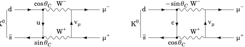
The fourth quark (charm) was proposed theoretically to explain the suppression of flavor changing neutral currents, such as the decay K0_→µ+µ−. The branching ratio

for this decay is 6.84_×10−9 _{[11], so clearly there is no first order contribution to}

this process. Even without first order flavor changing neutral currents, the decay K0_→µ+µ−should still be possible through a second order loop process, as shown on

the left in fig. 2.3. However, the expected branching ratio for this diagram is several orders of magnitude larger than the actual branching ratio.

Glashow, Iliopoulos and Maiani observed in 1970 that such processes could be suppressed if there was a fourth quark with the same charge as the u quark [12]. They extended Cabibbo’s mixing angle to a rotation matrix, which mixes down and strange quarks:

µ_d0

s0

¶

=

µ _cos

θ_C sinθ_C −sinθ_C cosθ_C

¶µ_d

s

¶

. (2.1)

The weak interaction then couples the u quark to d0and the new charm quark to s0. In processes with apparent flavor changing neutral currents, a second loop diagram has to be considered, which has a charm quark in the loop instead of an up quark (right diagram in fig. 2.3). Due to the minus sign in eq. (2.1), the two contributions cancel almost exactly, except for a small term due to the mass difference between the up and the charm quark. In addition, the unitarity of eq. (2.1) explains the absence of first order flavor changing neutral currents, since the rotated states d0and s0are orthogonal to each other.

The first meson containing charm quarks to be discovered was the J/ψ, which

is a bound cc state. In 1974 it was observed as a resonance at 3.1 GeV/c2 in two independent experiments: in the invariant mass spectrum of e+_e−_{pairs produced in}

collisions of protons on a beryllium target at BNL [13], and in the interaction cross section of e+e− beams at SLAC [14]. Charmed mesons consisting of a c quark and a light quark followed shortly afterwards.

d u s W− W+ µ+ ν_µ µ−

sinθ_C

cosθ_C

K0 d c s W− W+ µ+ ν_µ µ−

cosθ_C −sinθ_C

K0

Figure 2.3.: The process K0→µ+µ− is suppressed by the cancellation between two

(20)

2.1.4. Third family

The third lepton (τ) was discovered at SLAC shortly after the observation of the J/ψ.

Perl and collaborators reported 64 events with e+_e−_{in the initial state and an electron,}

a muon and missing energy in the final state [15]. Such a signature is explained by a pair of new leptons produced in the e+e−collision, with one lepton decaying to an electron and neutrinos, the other decaying to a muon and neutrinos.

For the quark sector, Kobayashi and Maskawa had suggested a third quark family already in 1973, before the charm quark and the τ were discovered, to explain the

origin of_CP violation [3]. With three families, the quark mixing matrix in eq. (2.1) is extended to a 3×3 matrix, which contains an irreducible complex phase. This phase is required to explainCP asymmetric processes, as will be shown in more detail in sections 2.3 and 2.4.

The Υ(1S), the first bound bb state analogous to the J/ψ, was found in 1977 at

Fermilab as a resonance at 9.5 GeV/c2 [16]. The last quark (top) turned out to be significantly heavier, with a rest mass of about 175 GeV/c2. In consequence, it was not discovered until 1995 [17, 18], when the Tevatron at Fermilab provided pp collisions with enough energy to produce top quark pairs.

2.2. Discrete symmetries

Symmetries play a fundamental role in physics. On the one hand, symmetries can often be exploited to simplify calculations and models, which might not be solvable at all otherwise. On the other hand, the observation of symmetries (or their absence) in nature provides insight into the underlying physical laws. In the following, the discrete symmetries_P,_C and_T are formally defined and the experimental history of

CP violation is given.

2.2.1. Parity inversion

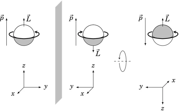
The parity inversion_P is defined as an inversion of all spatial coordinates. This is equivalent to a mirror reflection followed by a 180° rotation. After a parity inversion, the direction of motion of a particle (a vector) is reversed. However, the direction of the angular momentum and the spin (axial vectors) are unchanged, as illustrated in fig. 2.4.

The angular momentum part of a particle wave functionψ(~x) is an eigenstate of_P

(21)

2.2. Discrete symmetries 9

x y

z

~_L ~p

x y

z

~_L ~p

x y

z

~_L ~p

Figure 2.4.: A parity inversion is equivalent to a mirror reflection followed by a 180° rotation around the mirror axis. All spatial coordinates and the direction of motion~pare reversed. The angular momentum~Lis unchanged.

While the electromagnetic and the strong interaction conserve parity, the weak interaction violates it maximally. Historically, the first hint of parity violation was given by the observation of two particles, then namedθ+andτ+(not to be confused

with the τ lepton), which had the same mass and lifetime, but decayed to states of

different parity. In 1956 Lee and Yang suggested that theθ+andτ+might be the same

particle, which is called K+ _{today. They noted that parity conservation in the weak}

interaction had never been tested and proposed several experiments to do so [19]. In 1957 Wu and collaborators carried out one of the proposed experiments, which was based on theβdecay of polarized nuclei [20]. Angular momentum conservation

restricts the spins of the final state electron and neutrino to the direction of the spin of the decaying nucleus. A parity inversion would flip the momentum ~p of

the decay products, but not their spin~σ, in other words the helicity _|_~_p~p_|·|·~σ_~_σ_| is changed.

Therefore, an asymmetry in the angular distribution of the electrons with respect to the polarization axis implies a violation of parity symmetry. Indeed a clear asymmetry was observed and could be correlated to the polarization of the decaying nuclei, showing a maximal violation of parity symmetry. The result was confirmed shortly afterwards by Garwin, Lederman and Weinrich, who measured the polarization of muons produced in pion decays [21]. They found that the emitted muons were strongly polarized along the direction of motion, indicating again that parity symmetry is maximally violated.

2.2.2. Charge conjugation

(22)

angular momentum and spin are unchanged. A single particle state is an eigenstate of

C if it is its own antiparticle. For example, the neutral pion is an eigenstate ofC(C|π0_{〉 =}

|π0_〉), while the charged pions are transformed into each other by a charge conjugation

(_C|π±_{〉 = |}π∓_〉). A bound state of a fermion and the corresponding antifermion_|f f_〉is

an eigenstate of_C with eigenvalue (−1)L+S_{, where}_L_{is the angular momentum of the}

system and Sis the total spin, since the charge conjugation effectively exchanges the two particles. Other eigenstates of_C can be formed from the superposition of particle and antiparticle states.

A symmetry of charge conjugation would imply that particles and antiparticles behave identically. In other words, the charge conjugated equivalent of a process should happen with the same rate. As mentioned in the introduction, this assumption is in contradiction to the observed imbalance between matter and antimatter in the universe. Unless the asymmetry was present already at the Big Bang,C symmetry has to be violated at some point in the history of the universe.

In fact, C symmetry is also violated maximally in the weak interaction. This conclusion could be obtained from the same experiments that showedP symmetry violation, based on the fact that the combined symmetry of_CPT has to be conserved as a consequence of Lorentz invariance [22]. For example, the helicity of antimuons produced in pion decays is reversed compared to muons. Note, however, thatCviolation alone does not explain the matter-antimatter asymmetry. Further necessary conditions include the violation of baryon number conservation, interactions out of thermal equilibrium and the violation of the combinedCP symmetry [1].

2.2.3. Time reversal

The time reversal operationT transforms a process into one that is happening back-ward in time, that is it replacest→ −t. Position and charge of particles are unchanged, but the direction of motion and the angular momentum are reversed.

Macroscopically, the world is clearly not T symmetric, since the second law of thermodynamics states that entropy increases with time. However, microscopic processes are generally _T symmetric. As an example for a _T symmetric process in classical mechanics, consider the motion of a billiard ball bouncing off a wall. A backward recording of the motion follows the same equations of motion, so it would not be possible to decide if the recording is played forward or backward. If the ball hits another ball at rest, or if more than two balls are involved, we could distinguish the forward and backward motion with reasonable confidence. However, it is important to note that the backward motion of two colliding billiard balls still does not violate any laws of motion. It is simply very difficult to prepare the exact initial conditions that result in one ball being at rest after the collision. If more than two balls are involved, the difficulty to prepare the initial conditions increases, although the backward process is still physically allowed.

(23)

2.2. Discrete symmetries 11

state evolves to a certain final state, another system prepared in the final state of the original system with reversed direction of motion will evolve to the original initial state. An example for aT symmetric process in particle physics are the reactions K−_p_→_K0_{n and its reverse K}0_n

→K−p, which happen with the same rate.

2.2.4. Combined charge parity symmetry

CandP violation were included into the theory of weak interaction by writing the weak interaction current as a sum of vector and axial vector terms with equal coefficients. In consequence, the weak interaction couples only to left-handed fermions and right-handed antifermions, where left-(right-)right-handed means that the spin of a massless particle is antiparallel (parallel) to the direction of motion (for a massive particle the definition is more abstract, since the direction of motion depends on the reference frame). SoC andP are maximally violated separately, but the theory is symmetric with respect to the combined transformation of parity inversion and charge conjugation

CP.

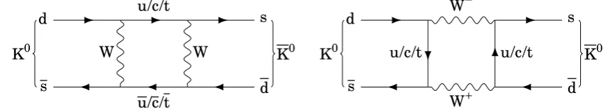
The violation ofCP symmetry was first observed in the neutral K0meson system. The K0 (ds) can be distinguished from its antiparticle K0 (ds) by their respective strangeness. However, a K0 can make a transition to a K0 and vice-versa by weak interaction processes, as shown in fig. 2.5. This allows the two states to mix coherently, that is the eigenstates of the weak interaction K0₁and K0₂ (states of definite mass and lifetime, also calledmass eigenstates) are a superposition of the flavor eigenstates K0and K0. Assuming that the weak interaction conservesCP, the mass eigenstates would also be eigenstates of the_CP operator:

|K01〉 =p1

2

³

|K0〉 + |K0〉´ CP|K01〉 = +|K01〉,

|K02〉 =p1

2

³

|K0〉 − |K0〉´ CP|K02〉 = −|K02〉.

The K0₁ decays dominantly to two pions in s-wave (with total angular momentum 0), which form a _CP even state. Still assuming that _CP is conserved, this decay

d u/c/t s

s

u/c/t d

W W

K0 K0

d

u/c/t s

s

u/c/t

d W+

W−

K0 K0

(24)

is forbidden for the K0₂, which decays to a _CP odd state with three pions instead. Since the mass of the kaon is only slightly higher than the mass of three pions, the latter process is strongly suppressed kinematically. Therefore, the lifetime of the K0₂ of 5.116_×10−8_{s is three orders of magnitude larger than the lifetime of the K}0

1 of

8.954×10−11_{s [11].}

In 1964 Christenson, Cronin, Fitch and Turlay made use of this lifetime difference to find evidence for the decay of the K0₂into two pions [2], proving that_CP symmetry is violated. They prepared a kaon beam which initially contains a mixture of K0₁ and K0₂ and let it travel until all K0₁ had decayed. Then they searched for a decay of the remaining K0₂ into two pions with an invariant mass that matches the mass of the kaon. Indeed they found two pion events from K0₂decays [2].

In contrast to P and C, the combined symmetry CP is only slightly violated in the weak interaction. Therefore, the true eigenstates of the weak interaction are almost identical to the K0₁and K0₂, but with a small contribution from the opposite_CP eigenstate. They are called K_S (“short” lived) and K_L (“long” lived) and are given by

|K_S〉 = |K01〉 +ε_|K0_{2〉 =}_p1

2

³

(1+ε)_{· |}K0_{〉 +}(1₋ε)_{· |}K0_〉´,

|K_L〉 =ε_|K0_{1〉 + |}K0_{2〉 =}_p1

2

³

(1+ε)_{· |}K0_{〉 −}(1₋ε)_{· |}K0_〉´.

Once the existence of_CP violation is accepted, it is necessary to quantify the contribu-tion of possible sources ofCP violation. For example, the parameterεis related to an

asymmetry between the transition probability from K0to K0 and the reverse process. It can be measured by comparing the decay rate of the K_L to flavor specific final states (states that identify the decaying kaon as either K0or K0), such as the semileptonic decays K0_→π−e+ν_e / K0_→π+e−ν_e. In addition, asymmetries in the decay process

itself can occur. Both effects are a consequence of a complex phase in the coupling parameter of the weak interaction, as will be shown in more detail in section 2.4.

2.3. CKM matrix

The coupling of the W bosons to quarks is described by the charged current Lagran-gian [23]

L_cc∝u_iγ_µ(1₋γ₅)V_{i j}d_jW+µ₊d_iγ_µ(1₋γ₅)V_{i j}†u_jW−µ

CP

−−→LCP

cc ∝djγµ(1−γ5)Vi juiW− µ

+u_jγ_µ(1₋γ₅)V_{i j}†d_iW+µ,

where the up-type quarksuare coupled to the down-type quarks dthrough the Dirac matricesγ_µ. The chirality operator (1₋γ₅) introduces parity asymmetry by projecting

to the left-handed component of the fermions. The unitary matrix V mixes

(25)

2.3. CKM matrix 13

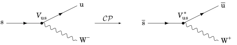
s

u

W−

Vus

s

u

W+

Vus∗ CP

Figure 2.6.: The coupling for the decay of a strange quark to an up quark is proporti-onal to the mixing matrix elementVus. In the charge conjugated decay

s_→u the complex conjugated elementV∗

us appears instead.

the two family mixing matrix in eq. (2.1). The three family version of the mixing matrix was proposed by Kobayashi and Maskawa in 1973 [3] and is now called the

Cabibbo-Kobayashi-Maskawa(CKM) matrixV_CKM, with corresponding quark tuples

u=(u,c,t) andd=(d,s,b).

Lccis invariant under aCP transformation ifVi j† =Vji, that is if the mixing matrix

is real. Conversely, this means that a_CP violating theory requires at least one non-trivial complex phase in the mixing matrix. Figure 2.6 illustrates the effect of a

CP transformation on a weak interaction vertex: the mixing matrix element that

appears in the coupling is replaced by its complex conjugate.

2.3.1. Parameters in a unitary matrix

A general unitaryn×n matrixU contains n2 free parameters. This can be seen for

example1 by noting thatU can be written as eiH, where H is hermitian. The total

number of free parameters of U and H is therefore the same. The parameters in

a hermitian matrix are easy to count: n real values on the diagonal plus 1₂n(n−1)

complex values above the diagonal give a total ofn2free parameters.

Unitarity requires that all column vectors ofU are normalized and orthogonal to

each other. This allows (n−1) degrees of freedom for the magnitude of the entries

in the first column, (n−2) for the second column and so on, giving 1₂n(n−1) real parameters in total, which are usually written as rotation angles. The remaining

1

2n(n+1) free parameters ofU are complex phases.

However, not all of these phases are physically observable. The LagrangianLccis

invariant under simultaneous transformations of

u_i→eiφi_u

i, dj→eiφjdj, Vi j→ei(φi−φj)Vi j.

The relative phases between such redefinitions can absorb (2n−1) phases in the mixing matrix [24]. An overall phase has no physical meaning and cannot cancel another phase in the matrix. This leaves 1₂(n−1)(n−2) physically observable phases with the

(26)

potential to cause _CP violation. For two families there are no such phases, which prompted Kobayashi and Maskawa to suggest a third family. In the CKM matrix (n=3) there is exactly one non-trivial phase.

2.3.2. Parametrization of the CKM matrix

There are various ways to define the CKM matrix, depending on the order of rotations and on the definition of the phase. A common definition is given by [24]

V_CKM₌

  

Vud Vus Vub

Vcd Vcs Vcb

V_td V_ts V_tb

 

=

  

c₁₂c₁₃ s₁₂c₁₃ s₁₃e−iδ −s₁₂c₂₃−c₁₂s₂₃s₁₃eiδ _c

12c23−s12s23s13eiδ s23c13

s₁₂s₂₃−c₁₂c₂₃s₁₃eiδ

−c₁₂s₂₃−s₁₂c₂₃s₁₃eiδ _c 23c13

 

,

where s_{i j} _≡sinθ_{i j} and c_{i j}_≡cosθ_{i j} are short for the sine and cosine of the rotation

angles andδis the single phase. A detailed derivation is given in [25], together with a

list of alternative representations.

Another useful representation is the Wolfenstein parametrization [26], which ex-pands the elements of the CKM matrix in terms of the parameterλ₌sinθ₁₂_≈0.22.

The angleθ₁₂ is the largest mixing angle in the CKM matrix and corresponds to the

Cabibbo angleθ_C in the two family model (eq. (2.1)). Noting the empirical relation |V_cb| ≈O(|V_us|2), Wolfenstein defined four parameters (λ,A,ρ,η) such that

λ₌sinθ₁₂, Aλ2₌sinθ₂₃, Aλ3(ρ₋iη)₌sinθ₁₃e−iδ.

Up to_O(λ3) the CKM matrix is then given by

V_CKM₌

  

1₋1₂λ2 λ Aλ3(ρ₋iη) −λ 1₋1₂λ2 Aλ2

Aλ3(1₋ρ₋iη) ₋Aλ2 1

 

+O(λ4). (2.2)

The advantage of this representation is that it directly reflects the hierarchy between the different elements: the largest coupling is found between quarks of the same family (O(1)), the second largest between the first and the second family (O(λ)), the third

largest between the second and the third family (_O(λ2)) and the smallest coupling is

found between the first and the third family (_O(λ3)). The complex phase appears only

in the smallest matrix elements and in higher order terms, reflecting the fact that

CP symmetry is only weakly violated in the standard model.

2.3.3. The unitarity triangle

(27)

2.3. CKM matrix 15

ℜ ℑ

(ρ,η)

VudVub∗

−V_cdV∗

cb =ρ+iη

(1,0)

VtdVtb∗

−VcdVcb∗ =1−ρ−iη

(0,0) VcdVcb∗

−V_cdV∗

cb = −1

φ₃ φ₂

φ₁

Figure 2.7.: Geometrically the unitarity condition eq. (2.7) can be represented as a triangle in the complex plane. The sides are normalized by₋V_cdV∗

cb, so by

definition two corners of the triangle are fixed at (0,0) and (1,0).

parametrization (eq. (2.2)), the unitarity conditionV_CKM† V_CKM₌1can be written up to O(λ3) as

¯ ¯ ¯Vud

¯ ¯

¯2+¯¯¯Vcd

¯ ¯

¯2+¯¯¯Vtd

¯ ¯

¯2=1=(1−λ2)₊λ2₊_O(λ4), (2.3)

¯ ¯ ¯Vus

¯ ¯

¯2+¯¯¯Vcs

¯ ¯

¯2+¯¯¯Vts

¯ ¯

¯2=1=λ2₊(1₋λ2)₊_O(λ4), (2.4)

¯ ¯ ¯Vub

¯ ¯

¯2+¯¯¯Vcb

¯ ¯

¯2+¯¯¯Vtb

¯ ¯

¯2=1=1+O(λ4), (2.5)

VudVus∗ +VcdVcs∗+VtdVts∗=0=(λ−1₂λ3)+(−λ+₂1λ3)+O(λ5), (2.6)

VudVub∗ +VcdVcb∗ +VtdVtb∗ =0=Aλ3(ρ+iη)−Aλ3+Aλ3(1−ρ−iη)+O(λ5), (2.7)

VusVub∗ +VcsVcb∗ +VtsVtb∗ =0=Aλ2−Aλ2+O(λ4). (2.8)

Six similar equations emerge from the conditionV_CKMV_CKM† ₌1. Equations (2.3) to (2.5)

are normalization conditions, while eqs. (2.6) to (2.8) are orthogonality conditions and constrain also the complex phase. Each of these conditions can be represented geometrically as a triangle in the complex plane. Of special interest is eq. (2.7), which contains three complex terms of order_O(λ3) that have to cancel perfectly, as shown

in fig. 2.7. By convention the triangle is normalized such that one side is purely real and has length 1. This fixes two corners of the triangle. The third corner2 can be determined by measuring the three angles and the length of the remaining two sides. Since the normalized triangle is fully defined by two parameters, this system is overconstrained and provides an excellent test of the Kobayashi Maskawa theory: the CKM Matrix is unitary only if the triangle closes.

2_{In the expansion up to}

O(λ3) the third corner corresponds to the Wolfenstein parameters (ρ,η). For

(28)

The triangle in fig. 2.7 is referred to as “the unitarity triangle” of the B meson system, since it is defined by the columnsVid andVib of the CKM matrix and thus

related to processes that involve B mesons. In principle, similar triangles can be defined for eqs. (2.6) and (2.8) if the Wolfenstein parametrization is extended to order

O(λ5). However, these triangles are almost degenerate, with one side being two

respectively four orders of magnitude smaller than the other sides. The degenerate triangles are related to K mesons (eq. (2.6)) and B_smesons (eq. (2.8)).

2.4. CP violation in the B meson system

CP violation can manifest itself in three different ways, which are illustrated in fig. 2.8:

1. _CP violation in decay, also called direct_CP violation, refers to decay processes that happen with a different rate than the charge conjugated process:

¯ ¯

¯〈f|B0〉¯¯¯26=¯¯¯〈f|B0〉¯¯¯2,

where|f〉is an arbitrary (semi)hadronic final state and|f〉 =CP|f〉 is the corre-spondingCP conjugated state.CP violation in decay can occur both for charged and for neutral mesons.

2. CP violation in mixing, also called indirectCP violation, occurs only for neutral mesons which can transform into each other, as discussed for the K0and K0in section 2.2.4. _CP violation in mixing refers to the case that the transition rate of a meson to the corresponding antimeson differs from the reciprocal process:

¯ ¯

¯〈B0|B0〉¯¯¯26=¯¯¯〈B0|B0〉¯¯¯2.

CP violation in decay

6=

B0 f B0 f

CP violation in mixing

B0 6= B0

interference between decays with and without mixing B0

B0

f 6= B0

B0

f

(29)

2.4. CP violation in the B meson system 17

If this is the case, the mass eigenstates of the neutral meson system are not identical with_CP eigenstates.

3. CP violation in the interference between decays with and without mixing, also called mixing-induced CP violation, can also be observed in neutral meson systems where the meson and antimeson mix coherently. If both flavor states can decay into the same final state, the decay amplitude is a coherent sum of the two flavor states. This type of process is therefore sensitive to a relative phase between the decay of a meson and the corresponding antimeson. _CP violation is observed if

¯ ¯

¯〈f|B0〉¯¯¯26=¯¯¯〈f|B0〉¯¯¯2,

where_|f〉is an arbitrary (semi)hadronic final state that is accessible from both

B0and B0(typically aCP eigenstate).

In the following, all of these processes are discussed for the B0 (bd) and its antipar-ticle B0(bd). For other meson systems, like the K0(sd), D0(cu) and B0_s (bs), the same principle phenomena occur, but the rates and timescales are very different depending on the mass and lifetime differences of the respective weak interaction eigenstates.

2.4.1. CP violation in decay

Consider the decay amplitude Af of a B0 to a final state f. In general, different

intermediate states contribute to the decay, so the decay amplitude can be written as a sum [23]

A_f =X i

¯

¯_a_i¯¯_ei(δ_i+φ_i)_.

Two types of phases appear here: the so-called weak phasesφ_i, which change sign

under aCP transformation, and the so-called strong phasesδ_i, which are invariant

under a_CP transformation. With this definition, the decay amplitude A_f of a B0to the charge conjugated final state f is given by

A_f =X i

¯

¯_a_i¯¯_ei(δ_i−φ_i)_.

(30)

b u

d d

W+

u

d

B0 π−

π+ b d

d d u/c/t u u B0 π− π+

Figure 2.9.: Tree diagram (left) and penguin diagram (right) for the decay B0→π+π−.

CP symmetry is violated if¯¯Af

¯ ¯₆₌¯¯_¯_A

f

¯ ¯

¯. This is equivalent to the condition

¯

¯_A_f¯¯2₋¯¯_¯_A

f

¯ ¯

¯2= −2X

i,j

¯

¯_a_i¯¯¯¯_a_j¯¯_sin(δ_i₋δ_j)sin(φ_i₋φ_j)₆₌0.

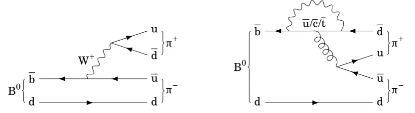
So CP violation in decay is only possible if at least two intermediate states with different weak and strong phases contribute to a decay. In other words, it is a consequence of the interference between states with different complex phases. In B decays, the relevant intermediate states are usually a “tree” diagram and a “penguin” diagram, as shown in fig. 2.9 for the decay B0_→π+π−. In this example, the CKM

matrix elements for both contributing diagrams are of order λ3, so the amplitudes

are of similar size. Therefore, a relatively large directCP violation is found [27]. In contrast, for decays that are dominated by a single diagram, direct _CP violation is very small.

The decay amplitudes¯¯_A_f¯¯2_and¯¯_¯_A

f

¯ ¯

¯2are proportional to the decay rates, so they

are directly accessible experimentally. However, the individual decay amplitudes ¯¯_a_i¯¯

and the strong phasesδ_i are very complicated to calculate theoretically and have large

uncertainties. Therefore, quantities that depend only on the weak phases provide much cleaner tests of the standard model.

2.4.2. CP violation in mixing

The neutral B0and B0mesons can transform into each other by diagrams analogous to fig. 2.5. The general state of such a system is given by a linear combination

|ψ_{〉 =}a_|B0_{〉 +}b_|B0_〉,

which evolves according to the time-dependent Schrödinger equation [23]

id dt µ a b ¶ =H µ a b ¶

=(M₋ i

2Γ)

µ

a b

¶

(31)

where M andΓ are hermitian matrices. Note that the total Hamiltonian H is not

hermitian, that is probability is not conserved. This reflects the fact that the total number of B0and B0is not constant, since the B mesons decay after some time. The diagonal elements of MandΓare related to the mass and lifetime of the pure flavor

eigenstates, respectively. As a consequence of_CPT invariance the B0and the B0 have the same mass and lifetime, which impliesH11=H22. The Hamiltonian can therefore

be written as

H₌

µ

M−₂iΓ M₁₂₋₂iΓ₁₂

M∗

12−2iΓ∗12 M−2iΓ

¶

.

The off-diagonal terms are responsible for the mixing and are thus related to box diagrams like the one in fig. 2.5 and to the CKM matrix. To find the mass eigenstates,

H is diagonalized, which gives the eigenvalues

mH/L−₂iΓH/L=M−₂iΓ±

sµ

M12−₂iΓ12

¶µ

M12∗ −₂iΓ∗12

¶

≡

µ

M±1₂∆m ¶

−₂i

µ

Γ_∓1

2∆Γ

¶

,

where mH/L andΓH/L are the mass and lifetime of the heavy (H) and light (L) mass

eigenstates and∆m₌m_H₋m_L and∆Γ₌Γ_L₋Γ_H are the differences between them.

By definition∆mis positive, while∆Γcan in principle be either positive or negative,

depending on the mixing matrix (for the K0system discussed in section 2.2.4, the K_S corresponds to the lighter mass eigenstate). The corresponding mass eigenstates are found to be

|BL〉 =p|B0〉 +q|B0〉, |B_H〉 =p|B0〉 −q|B0〉, with the coefficients obeying

q p= −

v u u

tM12∗ −2iΓ∗12

M12−2iΓ12

, |p|2+ |q|2=1.

CP violation occurs if¯¯¯q_p ¯ ¯

¯6=1, that is if the mass eigenstates are not alsoCP

eigensta-tes, as in the case of the K_L and K_S. This is only the case if the off-diagonal terms M₁₂

andΓ₁₂are of similar magnitude and at least one of them has a non-trivial complex

phase.

Another way to see that_CP symmetry is violated is to look at the time evolution of an arbitrary initial state|ψ_〉

|ψ(t₌0)_{〉 =}α_|B_L_{〉 +}β_|B_H_〉,

(32)

An initially pure flavor state_|B0_〉corresponds toα₌β₌_2p1 ; an initially pure_|B0_〉state

corresponds to α_{= −}β₌_2q1 . The time evolution is then given by

|B0(t)〉 =g+(t)|B0〉 + q_pg−(t)|B0〉,

|B0(t)〉 = p_qg₋(t)|B0〉 +g₊(t)|B0〉, (2.9)

g_±(t)₌1

2e−iMte−

1

2Γt³e2i∆mte−14∆Γt_±e−2i∆mte14∆Γt´.

So if¯¯¯q_p ¯ ¯

¯6=1, the probability to find an initial B0as a B0 at timetis not equal to the probability to find an initial B0 as a B0 after the same time. The time integrated probabilities then also differ. Experimentally these probabilities can be related to the decay rates of a B meson with known initial flavor state to a flavor specific final state.

In contrast to the K meson system, the lifetime difference∆Γin the B meson system

is much smaller than the mass difference∆m[23], since due to the large mass of the

B meson there are many more accessible final states than for the kaons. Similarly, for the off-diagonal matrix elements one findsΓ₁₂_¿M₁₂[28]. Therefore, to_O(10−2)

accuracy the following approximation holds:

q p= −

¯ ¯_M₁₂¯¯

M12 →

¯ ¯ ¯ ¯q_p

¯ ¯ ¯

¯≈1.

SoCP violation in mixing is very small in the B meson system. In this approximation, the mixing coefficients in eq. (2.9) can be simplified to

g±(t)=

1 2e−

iMt_e−1₂Γt³_e₂i∆mt

±e−2i∆mt´.

2.4.3. Interference between decays with and without mixing

When the final state of a B decay is accessible from both B0 and B0, both terms in eq. (2.9) contribute to the decay amplitude. Of special interest is the case where the final state is aCP eigenstate, that is

CP|fCP〉 = ±|fCP〉.

Denoting the decay amplitudes of a pure B0 (B0) to f_CP as A_CP (A_CP), the decay amplitudes after a timetcan be derived from eq. (2.9) as

A_CP(t)₌e−iMt_e−1₂Γt_A

CP Ã

cos∆mt 2 +i·

q p

A_CP A_CPsin

∆mt

2

!

,

A_CP(t)=e−iMte−12ΓtA

CPp_q

Ã

isin∆mt 2 +

q p

A_CP A_CPcos

∆mt

2

!

(33)

The_CP dependent parameters can be summarized in a single complex numberλ_CP,

which is defined as

λ_CP₌ q

p A_CP A_CP.

The time dependent decay rates are then given by

¯

¯_A

CP(t)

¯

¯2₌_e−Γt¯_¯_A

CP ¯ ¯2

Ã

1₊¯¯λ_CP¯¯2

2 +

1₋¯¯λ_CP¯¯2

2 cos(∆mt)− ℑ(λCP)sin(∆mt) !

,

¯ ¯

¯A_CP(t) ¯ ¯

¯2=e−Γt¯_¯_A

CP ¯ ¯2 ¯ ¯ ¯ ¯p_q

¯ ¯ ¯ ¯

2Ã₁₊¯_¯_λ

CP ¯ ¯2

2 −

1₋¯¯_λ CP

¯ ¯2

2 cos(∆mt)+ ℑ(λCP)sin(∆mt) !

.

A difference between the rates can be observed for t6=0 if λ_CP has a non-trivial

complex phase, even if¯¯λ_CP¯¯₌1, in other words if there is neither _CP violation in

decay nor CP violation in mixing. Furthermore, since the rates depend onℑ(λ_CP),

the complex phase can be measured explicitly. Note that it is essential to measure the time dependent rates. If the rates are integrated over time, the term sin(∆mt)

becomes 0 and all information about the phase ofλ_CP is lost.

With the approximation¯¯¯p_q¯¯¯2≈1, the time dependentCP asymmetry is given by

a_CP(t)_≡

¯

¯_A_CP₍_t₎¯¯2₋_¯¯¯_A_CP₍_t₎¯¯_¯2 ¯

¯_A_CP₍_t₎¯¯2₊_¯¯¯_A_CP₍_t₎¯¯_¯2 =

1−¯¯λ_CP¯¯2

1+¯¯λ_CP¯¯2cos(∆mt)−

2ℑ(λ_CP)

1+¯¯λ_CP¯¯2sin(∆mt). (2.10)

From this observable the parameter λ_CP can be directly extracted. So the task is

to measure the two decay rates ¯¯_A

CP(t)

¯

¯2 _and _|_A

CP(t)|2 as precisely as possible as

functions of time. Unfortunately, the B meson has many different decay channels, due to its high mass of 5.28 GeV/c2. Therefore, the branching fractions to specific

CP eigenstates are generally small, so a very large number of events is required. This motivates the construction of a dedicated B factory, which is designed to produce a large number of B and B mesons.

More precisely, B factories produce BB mesons in pairs, which originate from the decay of aΥ(4S) meson produced in an e+e− annihilation. Approximately 50 % of

these pairs consist of neutral B0B0 mesons, which are produced in the maximally entangled state

|ψ_{〉 =}_p1

2(|B

0_〉|_B0_{〉 − |}_B0_〉|_B0_〉_).

(34)

orthogonal to each other. The time evolution of the entangled system is given by

|ψ(t₁,t₂)_{〉 =}_p1

2(|B

0₍_t

1)〉|B0(t2)〉 − |B0(t1)〉|B0(t2)〉)

=p1

2e

−iM(t1+t2)_e−12Γ(t1+t2)_·

µ

cos

µ_∆_m₍_t

1−t2)

2

¶³

|B0B0〉 − |B0B0〉´

−isin

µ_∆_m₍_t

1−t2)

2

¶µ_p

q|B

0_B0_{〉 −} q

p|B

0_B0_〉¶¶_.

Until one particle decays t1=t2, so the term with two B mesons of the same flavor

vanishes. After the decay,t1and t2correspond to the respective decay times. From the

time evolved state|ψ(t₁,t₂)_〉 one can calculate the decay rate for one particle decaying

to the final state f1after a time t1and the other decaying to the final state f2after a

time t2.

To measure the time dependent_CP asymmetrya_CP, one looks for decays where one particle decays to aCP eigenstate f_CP at the time t_CP, while the other decays to a flavor specific final state ftagat the time ttag. The latter is called thetag side, as it

“tags” the flavor of both particles at the decay time ttag. If the tag side meson decays

first, theCP side meson is projected to the orthogonal flavor state at the momentttag.

If the_CPside meson decays first, att_CPthe_CPside meson was in the state that would have evolved to the flavor state orthogonal to ftag. Thus, the decay of two entangled

B mesons to the final states ftagand fCP is equivalent to the decay of a single B meson

with known flavor to the final state f_CP. Going through the full calculation of the two particle decay rate, one can rederive eq. (2.10), except that the time tis replaced by

t_CP−ttag[23]. Therefore, the most important observable for the measurement of time

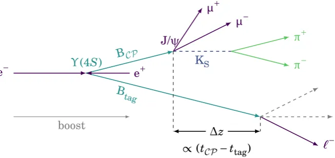
Υ(4S) BCP

B_tag

e− _e+

boost

`−

J/ψ

µ− µ+

K_S

π+

π−

∆z

∝(t_CP−ttag)

Figure 2.10.: Typical B0B0decay for the measurement of time dependent_CP violation. One B decays to a CP eigenstate (here J/ψK_S), the other decays to a

(35)

2.5. Open questions of the standard model 23

Events / 0.5 ps

0 50 100 150 200 250 300 350 400 t (ps) Δ

-6 -4 -2 0 2 4 6

Asymmetry -0.6 -0.4 -0.2 0 0.2 0.4 0.6

Events / 0.5 ps

0 50 100 150 200 250 t (ps) Δ

-6 -4 -2 0 2 4 6

Asymmetry -0.6 -0.4 -0.2 0 0.2 0.4 0.6

Figure 2.11.: Measured CP asymmetry in B0→(cc)K0 decays in the Belle experi-ment [29]. Shown are the background subtracted∆t distributions for

B_tag₌B0(red) and B_tag₌B0(blue) and the resulting asymmetrya_CP(∆t).

Left: combinedCP-odd decay modes, right: CP-even decay mode.

dependent_CP violation is the difference between the decay times of the two B mesons. To measure the oscillation in eq. (2.10), a timing resolution on the order of pico seconds is required. Since such small differences in the decay time cannot be measured, the Υ(4S) is produced with a boost, that is the colliding electrons and positrons

have different energies. Thus, the difference in the decay time is translated to a distance between the two decay vertices, which can be reconstructed more easily by precise silicon vertex detectors. The principle of the measurement is illustrated in fig. 2.10. The details about the boost of theΥ(4S) system are given in the next chapter.

Figure 2.11 shows the results of a time dependentCP violation measurement in the Belle experiment for theCP-odd decay B0→J/ψK_Sand related_CP-odd and_CP-even

decay channels with the same quark content. For this decay, the asymmetry at∆t₌0

is negligible, so there is no directCP violation, but in the time-dependent distribution there is a clear asymmetry, which is directly related to the angleφ₁of the unitarity

triangle shown in fig. 2.7 [29].

2.5. Open questions of the standard model

(36)

3 φ K ε 2 φ 2 φ d m

∆ ∆md & ∆ms

ub V 1

φ sin 2

(excl. at CL > 0.95) < 0

1

φ

sol. w/ cos 2

2 φ 1 φ 3 φ ρ

-0.4 -0.2 0.0 0.2 0.4 0.6 0.8 1.0

η 0.0 0.1 0.2 0.3 0.4 0.5 0.6 0.7

excluded area has CL > 0.95

ICHEP 16

CKM

f i t t e r

Figure 2.12.: Constraints on the unitarity triangle from measurements up to 2016 [30].

the angles and sides of the unitarity triangle, which are all compatible with each other within the present precision. However, there are many questions not answered by the standard model. One of them is how the asymmetry between matter and antimatter observed in the universe could arise. The measured_CPviolation is too weak to explain the asymmetry quantitatively. In addition, no baryon number violating processes are known in the standard model. Another problem is that the standard model has no explanation for dark matter and dark energy, which are necessary in cosmological models to explain the dynamics of galaxies and galaxy clusters and the expansion of the universe. Finally, the standard model does not include any description of gravity. Many theories have been proposed that extend the standard model, mostly by including new particles, interactions or symmetries. To discriminate between the different models, experiments need to observe some effect that is not in agreement with the standard model, which can give a hint at the underlying physics. There are two complementary experimental approaches. Experiments at the energy frontier, such as the Large Hadron Collider (LHC) at CERN, aim to create collisions at ever higher energies to find new heavy particles. In contrast, Belle II is an experiment at theintensity frontier, which searches for small deviations from the standard model predictions, using high statistics event samples.

(37)

2.5. Open questions of the standard model 25

Pohl, Sara (2018): Track reconstruction at the first level trigger of the Belle II experiment. Dissertation, LMU München: Fakultät für Physik

Track Reconstruction at the First Level

Trigger of the Belle II Experiment

Sara Pohl

Track Reconstruction at the First Level

Trigger of the Belle II Experiment

Sara Pohl

Dissertation

der Fakultät für Physik

der Ludwig-Maximilians-Universität

München

vorgelegt von

Sara Pohl (geb. Neuhaus)

aus Starnberg

Zusammenfassung

Abstract

Contents

1. Introduction

2.1. The standard model of particle physics

2.1.1. Light quarks

u

d

c

s

t

b

e

ν

µ

ν

τ

ν

γ

g

Z

W

H

2.1.2. Cabibbo angle

2.1.3. Charm quark

2.1.4. Third family

2.2. Discrete symmetries

2.2.1. Parity inversion

2.2.2. Charge conjugation

2.2.3. Time reversal

2.2.4. Combined charge parity symmetry

2.3. CKM matrix

2.3.1. Parameters in a unitary matrix

2.3.2. Parametrization of the CKM matrix

2.3.3. The unitarity triangle

2.4. CP violation in the B meson system

2.4.1. CP violation in decay

2.4.2. CP violation in mixing

2.4.3. Interference between decays with and without mixing

2.5. Open questions of the standard model