New Weaknesses in the Keystream Generation Algorithms of the Stream Ciphers TPy and Py

(1)

New Weaknesses in the Keystream Generation Algorithms of the

Stream Ciphers TPy and Py

∗

Gautham Sekar Souradyuti Paul Bart Preneel

Katholieke Universiteit Leuven, Dept. ESAT/COSIC, Kasteelpark Arenberg 10,

B–3001, Leuven-Heverlee, Belgium

{gautham.sekar, souradyuti.paul, bart.preneel}@esat.kuleuven.be

Abstract

The stream ciphers Py, Py6 designed by Biham and Seberry were promising candidates in the ECRYPT-eSTREAM project because of their impressive speed. Since their publication in April 2005, a number of cryptanalytic weaknesses of the ciphers have been discovered. As a result, a strengthened version Pypy was developed to repair these weaknesses; it was included in the category of ‘Focus ciphers’ of the Phase II of the eSTREAM competition. However, even the new cipher Pypy was not free from flaws, resulting in a second redesign. This led to the generation of three new ciphers TPypy, TPy and TPy6. The designers claimed that TPy would be secure with a key size up to 256 bytes, i.e., 2048 bits. In February 2007, Sekar et al.

published an attack on TPy with 2281

data and comparable time. This paper shows how to build a distinguisher with 2268

.6key/IVs and one outputword for each key (i.e., the distinguisher can be constructed within the design specifications); it uses a different set of weak states of the TPy. Our results show that distinguishing attacks with complexity lower than the brute force exist if the key size of TPy is longer than 268 bits. Therefore, for longer keys, our attack constitutes an academic break of the cipher. Furthermore, we discover a large number of similar bias-producing states of TPy and provide a general framework to compute them. The attacks on TPy are also shown to be effective on Py.

1 Introduction

Timeline: the Py-family of Ciphers

• April 2005. The ciphers Py and Py6, designed by Biham and Seberry, were submitted to the ECRYPT project for analysis and evaluation in the category of software based stream ciphers [2]. The impressive speed of the cipher Py in software (about 2.5 times faster than the RC4) made it one of the fastest and most attractive contestants. The cipher is designed to be used with a key of size 32 bytes (the key size may vary between 1 byte and 256 bytes) and an IV of size 16 bytes (the IV size can vary between 1 and 64 bytes).

• March 2006 (at FSE 2006). Paul, Preneel and Sekar reported distinguishing attacks with 289.2 _{data and comparable time against the cipher Py [7]. Crowley [4] later reduced the}

complexity to 272 _{by employing a Hidden Markov Model.}

∗_{The first author is supported by an IWT SoBeNeT project. The second author is funded by the IBBT}

(2)

• March 2006 (at the Rump session of FSE 2006). A new cipher, namely Pypy, was proposed by the designers to rule out the aforementioned distinguishing attacks on Py [3].

• May 2006 (presented at Asiacrypt 2006). Distinguishing attacks were reported against Py6 with 268.6 _{data and comparable time by Paul and Preneel [8].}

• October 2006 (to be presented at Eurocrypt 2007). Wu and Preneel showed key recovery attacks against the ciphers Py, Pypy, Py6 with chosen IVs [10]. This attack was subsequently improved by Isobeet al. [5].

• January 2007. Three new ciphers TPypy, TPy, TPy6 were proposed by the designers [1]. These three ciphers can very well be viewed as the strengthened versions of the previous ciphers Py, Pypy and Py6 where the above attacks do not apply. The ciphers are designed to be secure for any key size between 1 byte and 256 bytes.

• February 2007. Sekar et al. published an attack on TPy which requires 2281 _{data and}

comparable time [9].

In this paper, we show distinguishing attacks on the ciphers TPy and Py with data complexity 2268.6 _{each. These results outperform the most recent attack on TPy which requires 2}281 _{data [9].}

However, it is worth noting that the attacks described in [7] can also be applied to TPy. In the design specifications, the TPy and the Py are claimed to be compatible with key size ranging from 8 bits to 2048 bits. If the ciphers are used with key size longer than 268 bits then our attacks are better than exhaustive search. It is also worth noting that the distinguisher can be built within the design specifications of the ciphers. To derive the distinguisher, 2268.6 _{randomly chosen key/IVs}

are used and for each of them one outputword is collected. Note that, according to the design specification, TPy can run for 261 rounds (note that each round generates 8 bytes as output) per key where our distinguisher requires only 8 rounds per key.

In addition to the above distinguisher, we detect biases in a large number of outputs at rounds

r, r+ 2, t and u where r > 0; t, u≥ 5; t 6∈ {r, r+ 2, u}; u 6∈ {r, r+ 2, t}. We provide a general framework to compute the biases due to the presence of arbitrarily many weak states. However, we were unable to combine those biases into a more efficient attack. Combining multiple distinguishers into a single and more efficient one is still an alluring open problem.

2 The Round Function of TPy

The round functions of the TPy and the Py are identical. Here, we analyze only the round function of TPy and hence do not describe the key setup and IV setup. Algorithm 1 describes a single round of the TPy. Array P (which is a permutation of [0,1, ...,255]), array Y (which contains 260 32-bit elements) and the 32-bit variable s are the inputs to the algorithm. Here, ‘rotate(A)’ denotes a cyclic rotation of the elements of arrayAby one position. The ‘ROT L32(s, k)’ operation means that the 32-bit variable sis rotated to the left bykpositions. The output generated in line 5 of the algorithm is labeled ‘first output-word’ and the output-word of line 6 is labeled ‘second output-word’.

3 Notation and Convention

• O_a₍_b₎denotes thebth bit (b= 0 denotes the least significant bit or lsb) of the first output-word generated at round a. We do not use the second output-word anywhere in our analysis.

• Pa, Ya+1 and sa are the inputs to the algorithm at round a. It is easy to see that when

this convention is followed, Oa = (ROT L32(sa,25)⊕Ya[256]) +Ya[Pa[26]]- the index ‘a’ is

(3)

Algorithm 1 A Step of TPy

Require: Y[−3, ...,256],P[0, ...,255], a 32-bit variables

Ensure: 64-bit random output /*Update and rotateP*/

1: swap (P[0], P[Y[185]&255]);

2: rotate (P); /* Update s*/

3: s+ =Y[P[72]]−Y[P[239]];

4: s=ROT L32(s,((P[116] + 18)&31));

/* Output 8 bytes (least significant byte first)*/

5: output ((ROT L32(s,25)⊕Y[256]) +Y[P[26]]);

6: output (( s ⊕Y[−1]) +Y[P[208]]); /* Update and rotateY*/

7: Y[−3] = (ROT L32(s,14)⊕Y[−3]) +Y[P[153]];

8: rotate(Y);

• Ya[b], Pa[b] denote thebth elements of arrayYa and Pa respectively.

• Ya[b]i,Pa[b]i denote the ith bit (i= 0 denotes the lsb) of Ya[b],Pa[b] respectively.

• The operators ‘+’ and ‘−’ denoteaddition modulo232_and_{subtraction modulo}₂32_{respectively,}

except when used with expressions which relate two elements of array P. In this case they denote addition and subtraction over Z.

• The symbol ‘⊕’ denotes bitwiseexclusive-or and Tdenotes set intersection.

• InO_a₍_i₎,s_a₍_i₎ and Ya[Pb[X]]i, the index representing bit position, i.e.,idenotesimod 32. • Y_ac[Pb[X]]i denotes the complement ofYa[Pb[X]]i.

• The pseudorandom bit generation algorithm of a stream cipher is denoted by PRBG.

4 Motivational Observations

Our major observation is the detection of a relation between the elements of the internal state and the outputs of the TPy which can, eventually, be used to build a distinguishing attack on the cipher. The relation is outlined in the following theorem.

Theorem 1 O₁₍_i₎⊕O3(i+7)⊕O7(i+7)⊕O8(i+7)= 0if the following17conditions are simultaneously

satisfied.

1. P1[116]≡ −18 mod 32(event E1),

2. P2[116]≡7 mod 32 (eventE2),

3. P3[116]≡ −4 mod 32(event E3),

4. P7[116]≡3 mod 32 (eventE4),

5. P8[116]≡3 mod 32 (eventE5),

6. P1[72] =P2[239] + 1 (event E6),

(4)

8. P7[72] =P8[72] + 1 (event E8),

9. P7[239] =P8[239] + 1(event E9),

10. P3[72] = 254(event E10),

11. P₁[26] =P₃[239] + 2 (event E₁₁), 12. P1[72] = 3 (event E12),

13. P3[26] = 0 (event E13),

14. P1[239] =P7[26] + 6(event E14),

15. P7[153] = 252(event E15),

16. P₆[153] =P₈[26] + 2(event E₁₆),

17. d₇₍i−7)⊕d8(i−7)⊕c1(i)⊕d3(i)⊕d1(i+7)⊕c3(i+7)⊕c7(i+7)⊕e7(i+7)⊕c8(i+7)⊕e8(i+7)= 0 (event

E17).1

Proof. First, we state and prove two lemmata which will be used to establish the theorem.

Lemma 1 If

1. P1[116]≡ −18 mod 32,

2. P₃[116]≡ −4 mod 32, 3. P7[116]≡3 mod 32,

4. P8[116]≡3 mod 32

then the following equations are satisfied:

1. O₁₍_i₎=s₀₍_i₊₇₎⊕Y₁[P₁[72]]i+7⊕Y1c[P1[239]]i+7⊕Y1[256]i⊕Y1[P1[26]]i⊕c1(i)⊕d1(i+7),

2. O₃₍i+7)=s2(i)⊕Y3[P3[72]]i⊕Y3c[P3[239]]i⊕Y3[256]i+7⊕Y3[P3[26]]i+7⊕c3(i+7)⊕d3(i),

3. O₇₍_i₊₇₎=Y7[P7[72]]i−7⊕Y

c

7[P7[239]]i−7⊕Y6[−3]i+7⊕Y7[P7[26]]i+7⊕Y6[P6[153]]i+7⊕c7(i+7)

⊕d₇₍_i

−7)⊕e7(i+7),

4. O₈₍_i₊₇₎=Y₈[P₈[72]]i−7⊕Y

c

8[P8[239]]i−7⊕Y7[−3]i+7⊕Y8[P8[26]]i+7⊕Y7[P7[153]]i+7⊕c8(i+7)

⊕d₈₍_i₋₇₎⊕e₈₍_i₊₇₎.

Proof. From Figure 1, we get

Yn[i] =Yn+1[i−1] (1)

when −2≤i≤256. Wheni=−3,

Yn+1[256] = (ROT L32(si,14)⊕Yn[−3]) +Yn[Pn[153]].

Generalizing (1), we have

Yn[i] =Yn+k[i−k] (2)

when −3≤i−k≤255. Line 5 of Algorithm 1 gives

1_{The terms}_c_,_d_,_e_{are the carries generated in certain expressions, the descriptions of which can be found in the}

(5)

A B C

X

Y A1

Y B C

C

D

D E

A1 B1

Y _Y

Y

n n+1 n+2

−3 −2 −1

255 256

Figure 1: The figure shows the update of the S-box Y. Yn[i] = Yn+1[i−1] when −2 ≤i ≤ 256.

Yn+1[256] = A1 when i = −3 and A1 = (ROT L32(sn,14)⊕A) +Yn[Pn[153]]. Generalizing the

above, we can write Yn[i] =Yn+k[i−k] when −3≤i−k≤255.

O7 = (ROT L32(s7,25)⊕Y7[256]) +Y7[P7[26]]. (3)

Let thec₇ denote the carry in the above equation. Since ROT L32(s₇,25)i =s7(i−25 mod 32),

O₇₍_i₎ = s₇₍_i₋_{25 mod 32)}⊕Y7[256]i⊕Y7[P7[26]]i⊕c7(i). (4)

Lines 3 and 4 of Algorithm 1 give us

s7 = ROT L32(s6+Y7[P7[72]]−Y7[P7[239]], P7[116] + 18 mod 32) (5)

⇒s₇₍j) = s6(j−kmod 32)⊕Y7[P7[72]]j−kmod 32⊕Y

c

7[P7[239]]j−kmod 32⊕d7(j−kmod 32) (6)

where k =P7[116] + 18 mod 32, d7(i) =f7(i)⊕g7(i) and d7(0) = 1 (f7 and g7 are the carry terms

in (5) which are explained in Sect. 5.2). For simplicity, henceforth we denote X₍_i_{mod 32)} by X₍_i₎. Thus (6) becomes,

s₇₍_j₎ = s₆₍_j₋_k₎⊕Y7[P7[72]]j−k⊕Y

c

7[P7[239]]j−k⊕d7(j−k). (7)

Ifj =i−25 mod 32, then (7) becomes

s₇₍_i₋₂₅₎=s₆₍_i₋_k₋₂₅₎⊕Y7[P7[72]]i−k−25⊕Y

c

7[P7[239]]i−k−25⊕d7(i−k−25). (8)

Substituting (8) in (4), we get,

O₇₍_i₎=s₆₍_i₋_k₋₂₅₎⊕Y7[P7[72]]i−k−25⊕Y

c

7[P7[239]]i−k−25⊕Y7[256]i⊕Y7[P7[26]]i⊕c7(i)⊕d7(i−k−25). (9)

Next, we have

Y7[256] = (ROT L32(s6,14)⊕Y6[−3]) +Y6[P6[153]], (10)

Y7[256]i = s6(i−14)⊕Y6[−3]i⊕Y6[P6[153]]i⊕e7(i) (11)

wheree7 is the carry term in (10). Substituting (11) in (9), we get,

O₇₍_i₎ = s₆₍_i

−k−25)⊕s6(i−14)⊕Y7[P7[72]]i−k−25⊕Y

c

7[P7[239]]i−k−25⊕Y6[−3]i

⊕Y7[P7[26]]i⊕Y6[P6[153]]i⊕c7(i)⊕d7(i−k−25)⊕e7(i). (12)

Now, if k = −11 (i.e., k ≡ −11 mod 32 ⇒ P7[116] + 18 ≡ −11 mod 32 ⇒ P7[116] ≡ 3 mod 32)

thens₆₍_i₋_k₋₂₅₎⊕s₆₍_i₋₁₄₎= 0. Hence, whenP7[116]≡3 mod 32, (12) becomes

O₇₍_i₎ = Y₇[P₇[72]]i−14⊕Y

c

7[P7[239]]i−14⊕Y6[−3]i⊕Y7[P7[26]]i

(6)

By similar arguments, whenP8[116]≡3 mod 32,

O₈₍_i₎ = Y₈[P₈[72]]i−14⊕Y

c

8[P8[239]]i−14⊕Y7[−3]i⊕Y8[P8[26]]i

⊕Y7[P7[153]]i⊕c8(i)⊕d8(i−14)⊕e8(i). (14)

From (9), we get

O₁₍_i₎ = s₀₍_i₋_k₋₂₅₎⊕Y1[P1[72]]i−k−25⊕Y

c

1[P1[239]]i−k−25⊕Y1[256]i

⊕Y1[P1[26]]i⊕c1(i)⊕d1(i−k−25). (15)

When k= 0 (i.e.,P₁[116]≡ −18 mod 32), the above equation reduces to

O₁₍_i₎=s₀₍_i₊₇₎⊕Y1[P1[72]]i+7⊕Y1c[P1[239]]i+7⊕Y1[256]i⊕Y1[P1[26]]i⊕c1(i)⊕d1(i+7). (16)

Similarly, when P3[116]≡ −4 mod 32, we have

O₃₍i+7) =s2(i)⊕Y3[P3[72]]i⊕Y3c[P3[239]]i⊕Y3[256]i+7⊕Y3[P3[26]]i+7⊕c3(i+7)⊕d3(i). (17)

From (13) and (14), we derive the following results:

O₇₍_i₊₇₎ = Y7[P7[72]]i−7⊕Y

c

7[P7[239]]i−7⊕Y6[−3]i+7⊕Y7[P7[26]]i+7⊕Y6[P6[153]]i+7⊕c7(i+7)

⊕d₇₍_i₋₇₎⊕e₇₍_i₊₇₎, (18)

O₈₍_i₊₇₎ = Y8[P8[72]]i−7⊕Y

c

8[P8[239]]i−7⊕Y7[−3]i+7⊕Y8[P8[26]]i+7⊕Y7[P7[153]]i+7⊕c8(i+7)

⊕d₈₍i−7)⊕e8(i+7). (19)

This completes the proof.

Now we state the second lemma.

Lemma 2 s₀₍i+7)=s2(i) if the following conditions are simultaneously satisfied,

1. P1[116]≡ −18 mod 32,

2. P2[116]≡7 mod 32,

3. P1[72] =P2[239] + 1,

4. P1[239] =P2[72] + 1.

Proof. Equation (5) gives us:

s₁ = ROT L32(s₀+Y₁[P₁[72]]−Y₁[P₁[239]], P₁[116] + 18 mod 32).

The first condition (P1[116]≡ −18 mod 32) reduces this to

s1 = s0+Y1[P1[72]]−Y1[P1[239]].

Therefore,

s₂ =ROT L32(s₀+Y₂[P₂[72]]−Y₂[P₂[239]] +Y₁[P₁[72]]−Y₁[P₁[239]], P₂[116] + 18 mod 32).

Conditions 3 and 4 reduce the above equation to

(7)

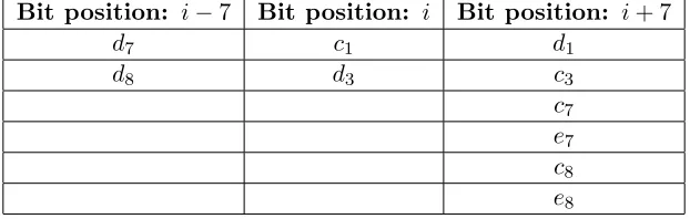
Table 1: Terms generated inO₁₍i)⊕O3(i+7)⊕O7(i+7)⊕O8(i+7), when eventsE1toE7simultaneously

occur, grouped by their bit positions

Bit position: i−7 Bit position: i Bit position: i+ 7

Y7[P7[72]] Y1[256] Y1[P1[72]]

Y7[P7[239]] Y1[P1[26]] Y1[P1[239]]

Y8[P8[72]] Y3[P3[72]] Y3[256]

Y8[P8[239]] Y3[P3[239]] Y3[P3[26]]

Carries Carries Y6[P6[153]]

Y6[−3]

Y7[P7[26]]

Y7[P7[153]]

Y7[−3]

Y₈[P₈[26]] Carries

Finally, with condition 2 (i.e., P₂[116]≡7 mod 32), the previous equation becomes

s2 = ROT L32(s0,25)

⇒s₂₍_i₎ = ROT L32(s0,25)i =s0(i−25)

= s₀₍_i₊₇₎. (20)

Now we observe that, when the conditions listed under (i) Lemma 1 (i.e., eventsE1,E3,E4 andE5)

and (ii) Lemma 2 (i.e., eventsE₁,E₂,E₆ and E₇) are simultaneously satisfied, then the expression

O₁₍_i₎⊕O₃₍_i₊₇₎⊕O₇₍_i₊₇₎⊕O₈₍_i₊₇₎ is the XOR of the terms which are listed in Table 1 (grouped according to the bit positions).2 Similarly, the ‘carries’ in Table 1 are elaborated in Table 2.

Table 2: Carry terms generated inO₁₍_i₎⊕O₃₍_i₊₇₎⊕O₇₍_i₊₇₎⊕O₈₍_i₊₇₎ grouped by their bit positions

d7 c1 d1

d8 d3 c3

c7

e7

c8

e8

If theY-terms in Table 1 are pairwise equated (this is achieved when the eventsE₈ through to

E16 occur) then we get

O₁₍_i₎⊕O₃₍_i₊₇₎⊕O₇₍_i₊₇₎⊕O₈₍_i₊₇₎ = d₇₍_i

−7)⊕d8(i−7)⊕c1(i)⊕d3(i)⊕d1(i+7)⊕c3(i+7)⊕c7(i+7)⊕e7(i+7)

⊕c₈₍_i₊₇₎⊕e₈₍_i₊₇₎. (21)

2_{Note that none of the terms listed in Table 1 is of the form}_Ac

because we used the fact thatAc

⊕Bc

=A⊕B

(8)

Now, when the RHS of (21) equals zero (i.e.,E17 occurs) we get

O₁₍_i₎⊕O₃₍_i₊₇₎⊕O₇₍_i₊₇₎⊕O₈₍_i₊₇₎= 0.

5 Computation of the Bias

In this section, we quantify the bias in the outputs of TPy induced by the fortuitous events similar to the one described in Sect. 4. Now it is important to note that there may bemore than one set of 17 conditions possible, where each of them results inO₁₍i)⊕O3(i+7)⊕O7(i+7)⊕O8(i+7)= 0 (let us

assume that there arensuch sets). In Theorem 1, we listed one such set. Our experiments suggest that thesen sets are mutually independent, however, a formal proof of that is nontrivial.

Each of the events E1 to E5 occurs with approximate probability ₃₂1 and each of the events

E6 to E16 occurs with probability which is approximately ₂₅₆1 . Let p denote the probability that

condition 17 is satisfied. Let F denote the eventT16_j₌₁Ej. Therefore,

P[F] = (1 32)

5_·₍ 1

256)

11_.

We see that there are n F-like events (i.e., the intersection of 16 conditions). Let Fn denote the

union of thesenevents. Since, each event occurs with approximately the same probability,

P[Fn] ≈ n·P[F] ≈ n·( 1

32)

5_·₍ 1

256)

11

= n· 1

2113.

From Table 1, we get the maximum number of ways that terms of a particular column can be pairwise equated and hence the upper bound on ncan be calculated to be 2·2·945 = 3780, that is,n <3780.

5.1 Formulating the Bias

Now, we establish a formula to compute P[O₁₍i) ⊕O3(i+7) ⊕O7(i+7)⊕O8(i+7) = 0], under the

assumption of a perfectly random key/IV setup and the uniformity of bits when Fn does not

occur.Our experiments suggest that it is infeasible to find a set of conditions such that the overall bias (computed on the basis of the aforementioned assumption of randomness in the event thatFn

does not occur) is canceled or reduced in magnitude. Therefore, this assumption is reasonable. Let

T denote O₁₍_i₎⊕O₃₍_i₊₇₎⊕O₇₍_i₊₇₎⊕O₈₍_i₊₇₎. Then using Bayes’ rule we get

P[T = 0] = P[T = 0|Fn∩E17]·P[Fn∩E17] +P[T = 0|Fnc∪E17c ]·P[Fnc∪E17c ]

= P[T = 0|Fn∩E17]·P[Fn∩E17] +P[T = 0|Fnc∩E17]·P[Fnc∩E17]

+ P[T = 0|Fn∩E17c ]·P[Fn∩E17c ] +P[T = 0|Fnc∩E17c ]·P[Fnc∩E17c ]

= 1·(n·p· 1

2113) +

1

2 ·(1−n· 1

2113)·p+ 0·P[Fn∩E

c

17] +

1

2·(1−n· 1

2113)·(1−p)

= 1

2 +n·(2p−1)· 1

2114. (22)

Hence, we see that the distribution of the outputs (O₁₍_i₎, O₃₍_i₊₇₎, O₇₍_i₊₇₎, O₈₍_i₊₇₎) is biased. The bias is equal to n·(2p−1)·₂1141 . In the following section, we provide formulas to compute p, i.e.,

the probability thatE17 occurs; or more generally, the probability that the 17th condition of each

(9)

5.2 Biases in the Carry Terms

In this section, we provide formulas to calculate the bias in the carry terms. The carry termscand

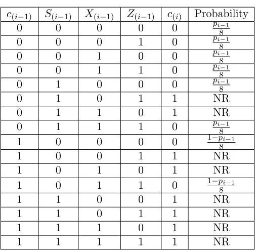
eare generated in expressions of the form (S⊕X) +Z. We now proceed to calculate P[c_l₍_i₎ = 0] assuming that S, X and Z are uniformly distributed and independent. Under this assumption,

P[Si = 0] = P[Xi = 0] = P[Zi = 0] = 1₂, that is, the probability that the carry bit at position i equals zero depends only on i. Stated otherwise, P[c₍_i₎ = 0] = P[e₍_i₎ = 0]. Let P[c₍_i₎ = 0] be denoted by pi. Since there is no carry on the lsb,p0 = 1. We now have Table 3.

Table 3: Truth table for computing pi (NR=Not Required)

c₍_i₋₁₎ S₍_i₋₁₎ X₍_i₋₁₎ Z₍_i₋₁₎ c₍_i₎ Probability

0 0 0 0 0 pi−1

8

0 0 0 1 0 pi₋₁

8

0 0 1 0 0 pi₋₁

8

0 0 1 1 0 pi₋₁

8

0 1 0 0 0 pi₋1

8

0 1 0 1 1 NR

0 1 1 0 1 NR

0 1 1 1 0 pi₋1

8

1 0 0 0 0 1−pi−1

8

1 0 0 1 1 NR

1 0 1 0 1 NR

1 0 1 1 0 1−pi₋1

8

1 1 0 0 1 NR

1 1 0 1 1 NR

1 1 1 0 1 NR

1 1 1 1 1 NR

From Table 3, using Bayes’ rule we get

pi = pi−1

2 + 1 4. Solving this recursion, givenp0 = 1, we get

pi =

1 2+

1

2i+1. (23)

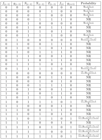
Now, the carry terms f and g are generated in expressions of the form S+X−Z. This can be rewritten as S +X +Zc + 1 since the additions in these two expressions are modulo 232_{. The}

presence of two carries inS+X+Z is demonstrated using the Figure 2. The carries generated in

S+X+Zc_{+ 1 can be thought of as carries generated in}_S₊_X₊_A_where_A₌_Zc _{and the carries}

on the lsb f₍₀₎ = 1, g₍₀₎ = 0. Let qi denote P[f(i) = 0] andri denote P[g(i) = 0]. Hence, q0 = 0,

r0 = 1 and r1 = 1. Now we have Table 4.

From Table 4, using Bayes’ rule we get

qi =

1 2+

5·qi−1·ri−1

8 −

qi−1

4 −

ri−1

4 , (24)

ri+1 = 1

2−

qi−1·ri−1

4 +

3·qi−1

8 +

3·ri−1

8 . (25)

(10)

Table 4: Truth table for computing qi andri+1 usingqi−1 andri−1 (NR=Not Required)

f₍_i

−1) g(i−1) S(i−1) X(i−1) Z(i−1) f(i) g(i+1) Probability

0 0 0 0 0 0 0 qi₋1·ri₋1

8

0 0 0 0 1 0 0 qi₋1·ri₋1

8

0 0 0 1 0 0 0 qi₋1·ri₋1

8

0 0 0 1 1 1 0 NR

0 0 1 0 0 0 0 qi−1·ri−1

8

0 0 1 0 1 1 0 NR

0 0 1 1 0 1 0 NR

0 0 1 1 1 0 0 qi₋_1·ri₋₁

8

0 1 0 0 0 0 0 qi₋1·(1−ri₋1)

8

0 1 0 0 1 1 0 NR

0 1 0 1 0 1 0 NR

0 1 0 1 1 1 0 NR

0 1 1 0 0 1 0 NR

0 1 1 0 1 1 0 NR

0 1 1 1 0 1 0 NR

0 1 1 1 1 0 1 qi₋_1·(1₋ri₋₁)

8

1 0 0 0 0 0 0 (1−qi₋₁)_·ri₋₁

8

1 0 0 0 1 1 0 NR

1 0 0 1 0 1 0 NR

1 0 0 1 1 1 0 NR

1 0 1 0 0 1 0 NR

1 0 1 0 1 1 0 NR

1 0 1 1 0 1 0 NR

1 0 1 1 1 0 1 (1−qi−1)·ri−1

8

1 1 0 0 0 1 0 NR

1 1 0 0 1 1 0 NR

1 1 0 1 0 1 0 NR

1 1 0 1 1 0 1 (1−qi₋1)·(1−ri₋1)

8

1 1 1 0 0 1 0 NR

1 1 1 0 1 0 1 (1−qi₋1)·(1−ri₋1)

8

1 1 1 1 0 0 1 (1−qi−1)·(1−ri−1)

8

1 1 1 1 1 0 1 (1−qi−1)·(1−ri−1)

(11)

g

f

0 0 1 1 1 1 0 1

1 1 0 1 1 1 1 0 0 1 1 1

0 1 0 1 + + 0 0 1 0 1 0 1+1+1=(3) 10=( 0 1 1 )2 0 1 0 1 0 0+0+ 0 1 0 0 1 Carries 1 0 0 0 1 1 1 0

( modulo 256)

S= 61

X= 221

SUM= 113

Z=87

Figure 2: An example showing how the carries are generated when three 8-bit variables S = 61,

X= 221 andZ = 87 are added

1. P[d₇₍_i

−7) = 0] =P[d8(i−7) = 0] =qi−7 mod 32·ri−7 mod 32

+ (1−qi−7 mod 32)·(1−ri−7 mod 32),

2. P[c₁₍_i₎= 0] = 1₂ +₂i1+1,

3. P[d₃₍_i₎ = 0] =qi·ri+ (1−qi)·(1−ri),

4. P[d₁₍_i₊₇₎ = 0] =qi+7 mod 32·ri+7 mod 32

+ (1−qi+7 mod 32)·(1−ri+7 mod 32),

5. P[c₃₍_i₊₇₎= 0] =P[c₇₍_i₊₇₎ = 0] =P[e₇₍_i₊₇₎ = 0] =P[c₈₍_i₊₇₎ = 0] =P[e₈₍_i₊₇₎= 0] = 1₂ + 1

2(i_{+7 mod 32)+1}.

Using the above formulas, the value of p can be computed for any given i. Running simulation, we find that the maximum bias in the chosen outputs occurs when i = 25 which corresponds to

p= 0.5−2−34.2. Hence, (22) gives us

P[T = 0] = 1 2−

n

2147.2

⇒P[T = 1] = 1 2 +

n

2147.2,

when i= 25. Substitutingn= 3780 in the above equation, we get:

P[T = 1] = 1 2+

1

2135.3. (26)

This is an upper bound on the probability that the outputs (O₁₍i),O3(i+7),O7(i+7),O8(i+7)) of TPy

are biased. From Sect. 4, we found thatn≥1. From the previous discussion, we see thatn <3780. Hence, 1≤n <3780. If n= 1, then P[T = 1] = 1₂ +₂1471.2. Thus,

1 2(1 +

1

2146.2)≤P[T = 1]≤

1 2(1 +

1

2134.3). (27)

6 The Distinguisher

(12)

Corollary 1 If an event eoccurs in a distribution X with probability p and in Y with probability p(1 +q) then, if p = 1₂, O(_q12) samples are required to distinguish X from Y with non-negligible

probability of success.

In the present case, e is the event O₁₍₂₅₎⊕O₃₍₀₎⊕O₇₍₀₎⊕O₈₍₀₎ = 0, X is the distribution of the outputs O₁, O₃, O₇ and O₈ produced by a perfectly random keystream generator and Y is the distribution of the outputs produced by TPy. From (27),p= 1₂ and the highest value of q= ₂1341.3.

HenceO( 1

(2−134.₃

)2) =O(2

268.6_{) output samples are needed to construct the best distinguisher with}

a non-negligible probability of success. Note that this is an improvement by a factor of 212.4 _over

the data complexity of 2281 obtained in [9].

7 A Family of Distinguishers

In Sect. 4 we found that the outputs at rounds 1, 3, 7 and 8 are biased allowing us to build a distinguisher. It is found that there exist plenty of 4-tuples of biased outputs. The generalization is presented in the following theorem.

Theorem 2 The distribution of the outputs (O_r₍_i₎, O_r₊₂₍_i₊₇₎, O_t₍_i₊₇₎, O_u₍_i₊₇₎) of the TPy are biased for many suitably chosen (r, t, u)’s where r >0;t, u≥5; t6∈ {r, r+ 2, u}; u6∈ {r, r+ 2, t}.

The proof is similar to the proof furnished for Theorem 1, however, a detailed proof has been provided in the Appendix A. This allows us to construct a family of distinguishers for the cipher TPy. It seems possible to combine these huge number of distinguishers in order to construct one single efficient distinguisher; however, any concrete mathematical model to combine them is still an interesting open problem. Another major implication of the above generalization theorem is the fact that the TPy outputs will remain always biased no matter how many initial outputwords are discarded from the keystream.

8 Attacks on Py

The PRBG of the cipher Py is identical with that of TPy. The attacks described in the previous sections exploit the weaknesses in the PRBG of TPy only. Therefore, all the attacks are applicable to Py also.

9 Conclusions and Open Problems

The paper develops a family of distinguishers from the outputs (O_r₍_i₎,O_r₊₂₍_i₊₇₎,O_t₍_i₊₇₎, O_u₍_i₊₇₎) of TPy (and Py), where r > 0; t, u≥ 5; t 6∈ {r, r+ 2, u}; u 6∈ {r, r+ 2, t}. Note that the TPy is one of the strongest members of the Py-family of ciphers. The best distinguisher works with data complexity 2268.6 _{which records an improvement of a factor of 5404 over the previous attack. In}

addition, we detect a large number of bias-producing states of TPy and compute them in a general framework. It is reasonable to assume that these weak states can be combined to mount a more efficient attack on TPy; however, methods to combine many distinguishers into a single yet more efficient one is still an open problem. We were unable to find the exact value of the bias in the distribution of the outputs (O₁₍₂₅₎,O₃₍₀₎,O₇₍₀₎,O₈₍₀₎). We leave this as an open problem.

References

[1] E. Biham, J. Seberry, “Tweaking the IV Setup of the Py Family of Ciphers – The Ciphers Tpy, TPypy, and TPy6,” Published on the author’s webpage at

(13)

[2] E. Biham, J. Seberry, “Py (Roo): A Fast and Secure Stream Cipher using Rolling Arrays,”

ecrypt submission, 2005.

[3] E. Biham, J. Seberry, “Pypy (Roopy): Another Version of Py,” ecrypt submission, 2006. [4] P. Crowley, “Improved Cryptanalysis of Py,”Workshop Record of SASC 2006 - Stream Ciphers

Revisited, ECRYPT Network of Excellence in Cryptology, February 2006, Leuven (Belgium), pp. 52-60.

[5] T. Isobe, T. Ohigashi, H. Kuwakado M. Morii, “How to Break Py and Pypy by a Chosen-IV Attack,” eSTREAM, ECRYPT Stream Cipher Project, Report 2006/060.

[6] I. Mantin, A. Shamir, “A Practical Attack on Broadcast RC4,”Fast Software Encryption 2001

(M. Matsui, ed.), vol. 2355 ofLNCS, pp. 152-164, Springer-Verlag, 2001.

[7] S. Paul, B. Preneel, G. Sekar, “Distinguishing Attacks on the Stream Cipher Py,”Fast Software Encryption 2006 (M. Robshaw, ed.), vol. 4047 ofLNCS, pp. 405-421, Springer-Verlag, 2006. [8] S. Paul, B. Preneel “On the (In)security of Stream Ciphers Based on Arrays and Modular

Addition,”Asiacrypt 2006 (X. Lai and K. Chen, eds.), vol. 4047 ofLNCS, pp. 69-83, Springer-Verlag, 2006.

[9] G. Sekar, S. Paul, B. Preneel, “Weaknesses in the Pseudorandom Bit Generation Algorithms of the Stream Ciphers TPypy and TPy,” available athttp://eprint.iacr.org/2007/075.pdf. [10] H. Wu, B. Preneel, “Differential Cryptanalysis of the Stream Ciphers Py, Py6 and Pypy,”

Eurocrypt 2007 (to appear).

A

Proof of the Theorem 2

Claim 1 The distribution of the outputs (Or(i), Or+2(i+7), Ot(i+7), Ou(i+7)) of the TPy are biased

for many suitably chosen (r, t,u)’s wherer >0; t, u≥5; t6∈ {r, r+ 2, u}; u6∈ {r, r+ 2, t}.

Proof. First, we state and prove two lemmata which will be used to establish the theorem.

Lemma 3 If

1. Pr[116]≡ −18 mod 32, 2. Pr+2[116]≡ −4 mod 32,

3. Pt[116]≡3 mod 32, 4. Pu[116]≡3 mod 32

then the following equations are satisfied:

1. O_r₍_i₎=s_r₋₁₍_i₊₇₎⊕Yr[Pr[72]]i+7⊕Yrc[Pr[239]]i+7⊕Yr[256]i⊕Yr[Pr[26]]i⊕cr(i)⊕dr(i+7),

2. Or+2(i+7)=sr+1(i)⊕Yr+2[Pr+2[72]]i⊕Yrc+2[Pr+2[239]]i⊕Yr+2[256]i+7⊕Yr+2[Pr+2[26]]i+7

⊕c_r₊₂₍_i₊₇₎⊕d_r₊₂₍_i₎, 3. Ot(i+7) =Yt[Pt[72]]i−7⊕Y

c

t[Pt[239]]i−7⊕Yt−1[−3]i+7⊕Yt[Pt[26]]i+7⊕Yt−1[Pt−1[153]]i+7⊕ct(i+7)

⊕d_t₍_i₋₇₎⊕e_t₍_i₊₇₎, 4. Ou(i+7)=Yu[Pu[72]]i−7⊕Y

c

u[Pu[239]]i−7⊕Yu−1[−3]i+7⊕Yu[Pu[26]]i+7⊕Yu−1[Pu−1[153]]i+7⊕

c_u₍_i₊₇₎

⊕d_u₍_i

(14)

Proof. Line 5 of Algorithm 1 gives

Ot = (ROT L32(st,25)⊕Yt[256]) +Yt[Pt[26]], (28)

Letct denote the carry in the above equation. Since ROT L32(st,25)i =st(i−25),

O_t₍_i₎ = s_t₍_i

−25)⊕Yt[256]i⊕Yt[Pt[26]]i⊕ct(i). (29)

Lines 3 and 4 of Algorithm 1 give us

st=ROT L32(st−1+Yt[Pt[72]]−Yt[Pt[239]], Pt[116] + 18 mod 32), (30)

⇒s_t₍_j₎=s_t₋₁₍_j₋_k₎⊕Yt[Pt[72]]j−k⊕Y

c

t[Pt[239]]j−k⊕dt(j−k) (31)

where k = Pt[116] + 18 mod 32, dt(i) = ft(i)⊕gt(i) and dt(0) = 1 (ft and gt are the carry terms

in (30). Ifj =i−25 mod 32, then (31) becomes

st(i−25)=st−1(i−k−25)⊕Yt[Pt[72]]i−k−25⊕Y

c

t[Pt[239]]i−k−25⊕dt(i−k−25). (32)

Substituting (32) in (29), we get,

Ot(i) =st−1(i−k−25)⊕Yt[Pt[72]]i−k−25⊕Y

c

t[Pt[239]]i−k−25⊕Yt[256]i⊕Yt[Pt[26]]i⊕ct(i)⊕dt(i−k−25).(33)

Next, we have

Yt[256] = (ROT L32(st−1,14)⊕Yt−1[−3]) +Yt−1[Pt−1[153]], (34)

Yt[256]i = st−1(i−14)⊕Yt−1[−3]i⊕Yt−1[Pt−1[153]]i⊕et(i) (35)

whereet is the carry term in (34). Substituting (35) in (33), we get,

Ot(i) = st−1(i−k−25)⊕st−1(i−14)⊕Yt[Pt[72]]i−k−25⊕Y

c

t[Pt[239]]i−k−25⊕Yt−1[−3]i

⊕Yt[Pt[26]]i⊕Yt−1[Pt−1[153]]i⊕ct(i)⊕dt(i−k−25)⊕et(i). (36)

Now, ifk=−11 (i.e.,k≡ −11 mod 32⇒Pt[116] + 18≡ −11 mod 32⇒Pt[116]≡3 mod 32) then s_t

−1(i−k−25)⊕st−1(i−14)= 0. Hence, when Pt[116]≡3 mod 32, (36) becomes

O_t₍_i₎ = Yt[Pt[72]]i−14⊕Y

c

t[Pt[239]]i−14⊕Yt−1[−3]i⊕Yt[Pt[26]]i

⊕Yt−1[Pt−1[153]]i⊕ct(i)⊕dt(i−14)⊕et(i). (37)

By similar arguments, whenPu[116]≡3 mod 32, Ou(i) = Yu[Pu[72]]i−14⊕Y

c

u[Pu[239]]i−14⊕Yu−1[−3]i⊕Yu[Pu[26]]i

⊕Yu−1[Pu−1[153]]i⊕cu(i)⊕du(i−14)⊕eu(i). (38)

From (33), we get

Or(i) = sr−1(i−k−25)⊕Yr[Pr[72]]i−k−25⊕Y

c

r[Pr[239]]i−k−25⊕Yr[256]i

⊕Yr[Pr[26]]i⊕cr(i)⊕dr(i−k−25). (39)

When k= 0 (i.e.,Pr[116]≡ −18 mod 32), the above equation reduces to O_r₍_i₎ = s_r

−1(i+7)⊕Yr[Pr[72]]i+7⊕Y

c

r[Pr[239]]i+7⊕Yr[256]i⊕Yr[Pr[26]]i

(15)

Similarly, when Pr+2[116]≡ −4 mod 32, we have

O_r₊₂₍_i₊₇₎ = s_r₊₁₍_i₎⊕Yr+2[Pr+2[72]]i⊕Yrc+2[Pr+2[239]]i⊕Yr+2[256]i+7

⊕Yr+2[Pr+2[26]]i+7⊕cr+2(i+7)⊕dr+2(i). (41)

From (37) and (38), we derive the following results:

O_t₍_i₊₇₎ = Yt[Pt[72]]i−7⊕Y

c

t[Pt[239]]i−7⊕Yt−1[−3]i+7⊕Yt[Pt[26]]i+7

⊕Yt−1[Pt−1[153]]i+7⊕ct(i+7)⊕dt(i−7)⊕et(i+7), (42)

Ou(i+7) = Yu[Pu[72]]i−7⊕Y

c

u[Pu[239]]i−7⊕Yu−1[−3]i+7⊕Yu[Pu[26]]i+7

⊕Yu−1[Pu−1[153]]i+7⊕cu(i+7)⊕du(i−7)⊕eu(i+7). (43)

Now we state the second lemma.

Lemma 4 For r >0, s_r

−1(i+7)=sr+1(i) if the following conditions are simultaneously satisfied,

1. Pr[116]≡ −18 mod 32, 2. Pr+1[116]≡7 mod 32,

3. Pr[72] =Pr+1[239] + 1,

4. Pr[239] =Pr+1[72] + 1.

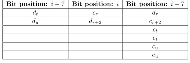
Table 5: Terms generated inO_r₍_i₎⊕O_r₊₂₍_i₊₇₎⊕O_t₍_i₊₇₎⊕O_u₍_i₊₇₎, when the conditions listed under Lemma 3 and Lemma 4 are simultaneously satisfied, grouped by their bit positions

Yt[Pt[72]] Yr[256] Yr[Pr[72]] Yt[Pt[239]] Yr[Pr[26]] Yr[Pr[239]]

Yu[Pu[72]] Yr+2[Pr+2[72]] Yr+2[256]

Yu[Pu[239]] Yr+2[Pr+2[239]] Yr+2[Pr+2[26]]

Carries Carries Yt−1[Pt−1[153]]

Yt−1[−3]

Yt[Pt[26]] Yu−1[Pu−1[153]]

Yu−1[−3]

Yu[Pu[26]]

Carries

Proof. Equation (30) gives us:

sr = ROT L32(sr−1+Yr[Pr[72]]−Yr[Pr[239]], Pr[116] + 18 mod 32).

The first condition (Pr[116]≡ −18 mod 32) reduces this to

sr = sr−1+Yr[Pr[72]]−Yr[Pr[239]].

Therefore,

(16)

Conditions 3 and 4 reduce the above equation to

sr+1 = ROT L32(sr−1, Pr+1[116] + 18 mod 32).

Finally, with condition 2 (i.e., Pr+1[116]≡7 mod 32), the previous equation becomes

sr+1 = ROT L32(sr−1,25)

⇒s_r₊₁₍_i₎ = ROT L32(sr−1,25)i =sr−1(i−25)=sr−1(i+7). (44)

Now we observe that, when the conditions listed under Lemma 3 and Lemma 4 are simultane-ously satisfied, then the expression O_r₍_i₎⊕O_r₊₂₍_i₊₇₎⊕O_t₍_i₊₇₎⊕O_u₍_i₊₇₎ is the XOR of the terms which are listed in Table 5 (grouped according to the bit positions).3 _{Similarly, the ‘carries’ in}

Table 5 are elaborated in Table 6. If theY-terms in Table 5 are pairwise equated, we get

Table 6: Carry terms generated inOr(i)⊕Or+2(i+7)⊕Ot(i+7)⊕Ou(i+7)grouped by their bit positions

dt cr dr

du dr+2 cr+2

ct et cu eu

O_r₍_i₎⊕O_r₊₂₍_i₊₇₎⊕O_t₍_i₊₇₎⊕O_u₍_i₊₇₎ = d_t₍_i₋₇₎⊕d_u₍_i₋₇₎⊕c_r₍_i₎⊕d_r₊₂₍_i₎⊕d_r₍_i₊₇₎

⊕cr+2(i+7)⊕ct(i+7)⊕et(i+7)⊕cu(i+7)⊕eu(i+7).(45)

Now, when the RHS of (45) equals zero, we get

O_r₍_i₎⊕O_r₊₂₍_i₊₇₎⊕O_t₍_i₊₇₎⊕O_u₍_i₊₇₎ = 0.

For a particular set of (r,t,u), we can have a set of 17 conditions similar to the set of conditions listed under Theorem 1, where r = 1, t = 7 and u = 8. In this way we can generate arbitrarily many (r, t,u)’s such that the outputs at rounds r, r+ 2, t and u are biased. This completes the

proof.

3_{Note that none of the terms listed in Table 5 is of the form}_Ac

because we used the fact thatAc

⊕Bc

=A⊕B