On the Complexity of Breaking Pseudoentropy
?Maciej Skorski??
IST Austria
Abstract. Pseudoentropy has found a lot of important applications to cryptography and complexity theory. In this paper we focus on the foun-dational problem that has not been investigated so far, namely by how much pseudoentropy (the amount seen by computationally bounded at-tackers) differs from its information-theoretic counterpart (seen by un-bounded observers), given certain limits on attacker’s computational power?
We provide the following answer for HILL pseudoentropy, which exhibits athreshold behavioraround the size exponential in the entropy amount:
– If the attacker size (s) and advantage () satisfy s2k−2 where
k is the claimed amount of pseudoentropy, then the pseudoentropy boils down to the information-theoretic smooth entropy
– Ifs2k2then pseudoentropy could be arbitrarily bigger than the information-theoretic smooth entropy
Besides answering the posted question, we show an elegant application of our result to the complexity theory, namely that it implies the clas-sical result on the existence of functions hard to approximate (due to Pippenger). In our approach we utilize non-constructive techniques: the duality of linear programming and the probabilistic method.
Keywords: nonuniform attacks, pseudoentropy, smooth entropy, hard-ness of boolean functions
1 Introduction
Pseudoentropy has recently attracted a lot of attention because of ap-plications to complexity theory [RTTV08], leakage-resilient cryptogra-phy [DP08,Pie09], deterministic encryption [FOR15], memory delega-tion [CKLR11], randomness extracdelega-tion [HLR07], key derivadelega-tion, [SGP15] constructing pseudorandom number generators [VZ12,YLW13] or black-box separations [GW11].
What differs between pseudoentropy and information-theoretic en-tropy notions is the parametrization by adversarial resources. That is,
?
The paper is available (with updates) athttps://eprint.iacr.org/2016/1186.pdf ??
pseudoentropy not only has quantity k but also quality, which is typi-cally described by the attacker sizesand the advantageachieved in the security game.
Despite many works on applications of pseudoentropy, not much is known about relationships between k, s and for a given distribution
X, in particular parameter settings that make pseudoentropy non-trivial (bigger than the information-theoretic entropy). Concrete numbers can be conjectured for some applications under assumptions about computa-tional hardness, for example for outputs of pesudorandom generators, or keys obtained by the Diffie-Hellman protocol. Yet in many cases, like key derivation where pseudoentropy can model “weak” sources [SGP15], one simply assumes pseudoentropy of certain (strong enough) quality.
Without understanding relations between s, and k it is not clear how demanding are specific assumptions on pseudoentropy quality. This is precisely the issue we are going to address in this work.
1.1 Problem statement
In this paper we are interested in separating pseudoentropy (entropy seen by computationally bounded attackers) from its information-theoretic counterpart (measured against unconstrained attackers).
Ann-bit random variable X is said to havekbits of pseudoentropy1 against attackers of size s and advantage if for some distribution Y of min-entropyk, no circuit of size scan distinguish it fromY with advan-tage bigger than(seeSection 2.4)2. Note that the notion is parametrized by the adversarial specific sizesand advantage. In particular the amount decreases when s gets bigger and gets smaller (it is harder to fool ad-versaries with bigger resources). When s is unbounded, pseudoentropy equals the information-theoretic smooth min-entropy (see Section 2.4).
To better understand possibilities and limitations of using pseudoen-tropy, it is natural to ask in what parameter regimes pseudoentropy pro-vides non-trivial computational security, that is when we have a real gain in the entropy amount comparing to the information-theoretic case.
Q: How much computational power is needed to boil pseudoen-tropy down to information-theoretic smooth enpseudoen-tropy?
1
We consider here the most popular notion of HILL pseudoentropy 2
1.2 Our Contribution
Nonuniform attacks against pseudoentropy Our result exhibit a threshold phenomena. Intuitively, with enough computational power (say size 2n for n-bit random variables3) the notion of pseudoentropy is no more stronger than the corresponding information-theoretic entropy no-tion. We estimate the value of this threshold on the circuit size s, so that above there is no computational gain and below there exists non-trivial pseudoentropy. There result is somewhat surprising because: (a) the threshold doesn’t depend on the length but the entropy amount and (b) the threshold depends also on the square of the advantage
Theorem (Informal) (Breaking pseudoentropy with enough com-putational power). For any k, and any s, satisfying
s2k−2
and for every distribution of min-entropy k, unbounded attackers and at-tackers of size s see the same entropy amount.
Theorem (Informal) (Lower bound). For any k, and any s, satis-fying
s2k2
there exists a distribution X such that
(a) (bounded attackers see k bits) pseudoentropy of X against circuits of size s and advantage is k
(b) (k bits for unbounded attackers see less than k bits) information-theoretic entropy of X is k
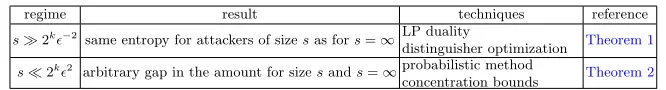
A short overview of our results is given in Table 1 below. We note that the result is tight with respect tok, but not with respect to .
regime result techniques reference
s2k−2 same entropy for attackers of sizesas fors=∞LP duality
distinguisher optimization Theorem 1
s2k2 arbitrary gap in the amount for sizesands=∞probabilistic method
concentration bounds Theorem 2
Table 1: Overview of our results. The analyzed setting is k bits of pseu-doentropy against size circuits of size sand advantage.
3
Proof outline and our tools
Breaking pseudoentropy We outline the proof of the first result below 1. We first consider somewhat weaker pseudoentropy notion, called
Met-ric entropy, where the order of quantifiers is reversed. That is, for any distinguisherDthere has to be someY of min-entropykwhich is close toX under that particular testD, that is ED(X)≈ED(Y).
2. We prove that this weaker pseudoentropy notion collapses whens
2k, by “compressing” distinguishers down to size 2k. The intuitive reason for that is that we can always manipulate Y so that it has “small” support (only O(2k) elements), and if an attacker wants to maximize the advantage |ED(X)−ED(Y)|, the best strategy is to hardcode the elementsxsuch that Pr[Y =x]>Pr[X=x] which is a subset of the support ofY and can be implemented in size ˜O(2k). 3. We use a generic transformation due to Barak at al. [BSW03,Sko15]
to go back to our standard entropy notion. The transformation losses ˜
O(2) in size and is based on the duality of linear programming. This way we obtain that pseudoentropy with parameters (s, ) becomes the same as the amount seen by unbounded attackers whens= ˜O 2k−2
. The details are explained in the proof of Theorem 1.
Matching lower bounds The proof of the second result goes as follows 1. We take a random subset X ⊂ {0,1}k of size k−c, where c will
be the gap between what bounded and unbounded attackers can see. The distributionX is the uniform distribution overX plus a “random shift” of an-fraction of the probability mass.
2. We argue that the -smooth entropy is still roughly k, because we have shifted only that fraction of the total probability mass. This is handled by a result of independent interest, stating that “almost” smooth distributions cannot be further smoothened (seeCorollary 2) 3. We argue that the distributionX is pseudorandom provided that the class of test functions is small enough. This fact is proved by applying concentration bounds twice, once to handle the random shift and for the second time to handle the choice ofX. Intuitively, the advantage of bounded attackers is much smaller than because they are “fooled” by the random shift of a part of the probability mass. In turn, the entropy amount seen by bounded attackers is much bigger thank−c
Putting this all together we get a strict separation: not only the amount of entropy is bigger, but also the advantage is smaller. The necessary assumption to make it work is that the class of distinguishers is much smaller than 22k−c2 members. For the details see the proof ofTheorem 2.
1.3 Related works
Pseudorandomness exists unconditionally The classical textbook results [Gol06] shows that pseudorandomness exists unconditionally, which can be seen as a separation between pseudorandomness and min-entropy.
OurTheorem 2is stronger as we separate pseudoentropy from smooth min-entropy (and cannot derive it from the mentioned result). From a technical point of view, the main difference is the extra random mass fluctuation (Step 1 in the above explanation), which needs to be later handled by bit more subtle probability tools (we use concentration in-equalities for random variables with local dependence due to Janson).
Complexity of non-uniform attacks against PRGs De, Trevisan and Tul-sani studied the complexity of nonuniform attacks against pseudorandom generators [DTT10]. Their results are specialized to outputs of PRGs and are constructive, whereas our results apply to any random variable (unfortunately don’t offer non-trivial results for the case of PRGs). Also,
1.4 Applications
Hard-to-approximate boolean functions Our Theorem 2implies the clas-sical result [Pip76] which states that for anyn and δ∈(0,1), there exist
δ-hard functions4 for sizes= ˜Ω 2n(1−δ)2
. For details, seeSection 5.1.
1.5 Organization
We start with explaining basic concepts and notions in Section 2. In
Section 3 we prove useful auxiliary facts about smooth min-entropy. In
Section 4 we give proofs of our main results. In Section 5 we discuss applications to the complexity of approximating boolean functions.
4
2 Preliminaries
2.1 Model of computations
Our results hold in the non-uniform model. We consider general classes of distinguishers, denoted byD, which are families of functions from nbits to real values. When discussing complexity applications, we restrictDto classes of circuits of certain size s, with boolean or real-valued outputs.
2.2 Basic notions
Definition 1 (Statistical distance). The statistical distance of two random variables X, Y taking values in the same finite set is defined as
SD(X, Y) = 12P
x|Pr[X = x]−Pr[Y = x]|. Equivalently, SD(X, Y) = maxD|ED(X)−ED(Y)|where D runs over all boolean functions.
2.3 Information-theoretic entropies
Definition 2 (Min-entropy).We say that Xhas kbits of min-entropy if minxlogPr[X1=x] =k.
Definition 3 (Smooth min-entropy [RW05]). We say that X has k
bits of -smooth min-entropy, denoted by H∞(X) >k, if X is -close in the statistical distance to some Y of min-entropy k.
Remark 1. Smoothing allows for increasing the entropy amount by shift-ing a part of the probability mass, to make the distribution look “more flat” or “more smooth”.
2.4 Pseudoentropy
In what follows, X denotes an arbitrary n-bit random variable.
Definition 4 (HILL pseudoentropy [HILL88,BSW03]). We say thatX has kbits of HILL pseudoentropyagainst a distinguisher class D
and advantage , denoted by
HHILLs, (X)>k
if there is a random variable Y of min-entropy at leastk that-fools any
Definition 5 (Metric Pseudoentropy [BSW03]).We say thatXhas
k bits of metric pseudoentropy against a distinguisher class D and ad-vantage , denoted by
HMetrics, (X)>k
if for any D∈ D there is a random variable Y of min-entropy at least k
that -fools this particular D that is such that|ED(X)−ED(Y)|6. Metric entropy is a convenient relaxation of HILL entropy, more suit-able to work with in many cases. The important fact below shows that both notions are equivalent up to some loss in the circuit size.
Lemma 1 (Metric-to-HILL Transformation [BSW03,Sko15]). If HMetrics, (X)>k thenHHILLs0,0 (X)>k where 0= 2and s0 ≈s2/n.
Remark 2 (Abbreviations and equivalences for circuit classes).In the spe-cific setting where D consists of deterministic boolean or deterministic real-valued circuits of sizeswe will slightly abuse the notation and write HMetrics, (X) =HMetricD, (X). This is justified by the fact that for metric en-tropy deterministic real-valued circuits of sizesgive the same amount as deterministic boolean circuits of sizes0 ≈s[FOR15]. In turn, for HILL en-tropy, deterministic boolean, deterministic randomized and deterministic real-valued circuits are equivalent with no entropy loss and with roughly same sizes [FOR15], so we also simply writeHHILLs, (X) =HHILLD, (X).
2.5 Relationships between entropy, smooth entropy, and computational entropy
The following proposition states that for extreme parameter regimes (un-bounded attackers or zero advantage), pseudoentropy collapses to the information-theoretic notion of smooth-entropy (we skip the easy proof).
Proposition 1. Let X be anyn-bit random variable. Then we have
(a) (Unbounded attackers) If s=∞5 then
HMetrics, (X) =HHILLs, (X) =H∞(X)>H∞(X) .
5
(b) (No smoothing) If = 0 then for any s
HMetrics, (X) =HHILLs, (X) =H∞(X) =H∞(X) .
(c) (General) For any s,
HMetrics, (X)>HHILLs, (X)>H∞(X)>H∞(X) .
2.6 Concentration inequalities
The following lemma is a corollary from the famous concentration bound due to Jason, which exploits local dependencies
Lemma 2 (Concentration bounds, local dependencies [Jan04]). Let X1, . . . , Xn be random variables with values in [a, b], such that ev-ery Xi is not independent of at most ∆ other variables Xi0. Let µ =
n−1Pn
i=1EXi. Then
Pr
"
n−1
n
X
i=1
Xi >µ+δ
#
6exp
− 2nδ
2
(a−b)2(∆+ 1)
.
In particular, for ∆= 0 we obtain the following bound
Corollary 1 (Hoeffding’s Inequality [Hoe63]). Let X1, . . . , Xn be independent random variables with values in[a, b]. Letµ=n−1Pn
i=1EXi.
Then
Pr
"
n−1
n
X
i=1
Xi>µ+δ
#
6exp
− 2nδ
2
(a−b)2
.
Remark 3 (Hoeffding’s Inequality for sampling without repetitions). The above inequality applies also the the setting whereXiare random samples taken from the same distribution without repetitions [Ser74].
3 Auxiliary Facts
3.1 Auxiliary results on smooth Renyi entropy
Lemma 3 (Flat distributions cannot be smoothened). Let X be an n-bit random variable. Suppose that the distribution of X is flat and H∞(X) =k. ThenH∞(X)6k+ log1−1 for every ∈(0,1).
Proof. Let X0 be any distribution of min-entropy at least k0 > k + log1−1 . Consider the distinguisher D which outputs D(x) = 1 if x ∈
supp(X) and D(x) = 0 otherwise. Note that ED(X) = 1 andED(X0) = supp(X)
2k0 <1−. ThereforeED(X)−ED(X
0) and thus the statistical dis-tance between X and X0 is bigger.
Corollary 2 (Almost-flat distributions cannot be smoothened). Suppose that X is1-close to some X0 being flat over 2k elements. Then
H2
∞(X)6k+ log
1 1−1−2
for any 1, 2>0 such that1+2<1.
Proof. Suppose not, then there exists X00 that is 2-close to X an has
min-entropy at least k0 > k+ log1−1
1−2
. In particular, X00 is -close to X0, where = 1 +2. Since X0 is flat, Lemma 3 implies that the
min-entropy ofX00 is at most k+ log
1 1−
, which is a contradiction.
4 Main Results
4.1 Complexity of breaking pseudoentropy
The following result specifies the attacker size for which pseudoentropy provides no computational security.
Theorem 1 (Breaking pseudoentropy is exponentially easy in the amount). For any n bit random variable X, if H∞(X) = k then also HHILLs, (X) =k for s > n22k−2.
The proof follows the steps explained in Section 1.2 and is given in
Appendix A.
4.2 Matching lower bounds
Theorem 2 (Breaking pseudoentropy can be exponentially hard in the amount). Let S ⊂ {0,1}nbe a set of cardinality 2k,0∈(0,1)be arbitrary, and let D be a class of functions from S to [0,1]such that
|D|<2−2·22k−C−102.
(a) HHILLD,0 (X) =k
(b) H∞(X) =k−C+ log1−12
Moreover, we have the following symmetry: the probability mass function of X takes only two values on two subsets of S of equal size.
Remark 4 (Doubly-strong separation: by the amount and the advantage). Note that the interesting setting of the parameters in the theorem above is when 0 so that not only we have a gap in the entropy amount, but even for much bigger advantage for unbounded distinguishers.
The proof follows the steps explained in Section 1.2 and appears in
Appendix B.
5 Applications
5.1 Complexity of hard boolean functions
For any functionf, and a distributionµon the domain off we denote by
GuessD(f, µ) the probability of guessingf by a functionDwhen the input is sampled according to µ, that is GuessD(f, µ) = Prx∼µ[D(x) =f(x)]. We say that f on nbits is δ-hard6 for sizes ifGuessD(f, µ) <1−δ2 for every circuitDof sizesand uniformµ(we also writeGuessD(f)<1−δ2). The corollary bellow is the classical result on the complexity of hard functions. Our result is optimal up to a factor linear in n(note that for largen, the value ofnis negligible comparing to 2n. Also, most interesting settings are with δ ≈ 1 with a negligible gap, and we get the optimal dependency on 1−δ.).
Corollary 3 (Functions hard to approximate by circuits).For any
nandδ ∈(0,1), there exists ann-bit function which isδ-hard for alln-bit boolean circuits of size s=Ω 2n(1−δ)2.
6
Proof (of Corollary 3). Let D0(x) = 2D(x) − 1. Denote for shortness
AdvD(X, Y) =ED(X)−ED(Y). Observe that for any X, Y we have AdvD(X, Y)
=ED(X)−ED(Y)
=1 2
X
x
(2D(x)−1) (Pr[X =x]−Pr[Y =x])
=SD(X, Y)Ex∼µD0(x)·sign(PX(x)−PY(x)) =SD(X, Y)
Pr x∼µ
D0(x) =f(x)− Pr x∼PX−PY
D0(x)6=f(x)
=SD(X, Y)
2 Pr x∼µ
D0(x) =f(x)
−1
=SD(X, Y)·2GuessD(f, µ)−1
wheref(x) =sign(PX(x)−PY(x)) and µ(x) = |PX(x)−PY(x)|
2SD(X,Y) (note that
P
xµ(x) = 1). Let us apply Theorem 2 to k = n, = 18,
0 = (1−δ) and D being the class of deterministic circuits of size s. Let Y be the indistinguishable distribution from the definition of HILL entropy. Since in our case Y is uniform, the function f is well-defined and moreover
SD(X, Y)>by (b). Thus
AdvD(X, Y)> ·2GuessD(f, µ)−1
Moreover, |PX(x)−PY(x)| is constant by construction. Therefore µ is uniform and we obtain
AdvD(X, Y)> ·2GuessD(f)−1
NowAdvD(X, Y)< (1−δ) impliesGuessD(f)<1−δ2 for anyD, which means that f is 1−δ-hard for sizes(here we use the fact that there are exponentially many circuits of size s, so that 2O(s) < 22k−O(1)(1−δ)2 and the assumption on the class size is satisfied).
.
References
CKLR11. Kai-Min Chung, Yael Tauman Kalai, Feng-Hao Liu, and Ran Raz,Memory delegation, Advances in Cryptology - CRYPTO 2011 - 31st Annual Cryptol-ogy Conference, Santa Barbara, CA, USA, August 14-18, 2011. Proceedings, 2011, pp. 151–168.
DP08. Stefan Dziembowski and Krzysztof Pietrzak,Leakage-resilient cryptography in the standard model, IACR Cryptology ePrint Archive2008(2008), 240. DTT10. Anindya De, Luca Trevisan, and Madhur Tulsiani, Time space tradeoffs for attacks against one-way functions and prgs, Advances in Cryptology -CRYPTO 2010, 30th Annual Cryptology Conference, Santa Barbara, CA, USA, August 15-19, 2010. Proceedings, 2010, pp. 649–665.
FOR15. Benjamin Fuller, Adam O’neill, and Leonid Reyzin,A unified approach to deterministic encryption: New constructions and a connection to computa-tional entropy, J. Cryptol.28(2015), no. 3, 671–717.
Gol06. Oded Goldreich, Foundations of cryptography: Volume 1, Cambridge Uni-versity Press, New York, NY, USA, 2006.
GW11. Craig Gentry and Daniel Wichs, Separating succinct non-interactive argu-ments from all falsifiable assumptions, Proceedings of the 43rd ACM Sym-posium on Theory of Computing, STOC 2011, San Jose, CA, USA, 6-8 June 2011, 2011, pp. 99–108.
HILL88. Johan H˚astad, Russell Impagliazzo, Leonid A. Levin, and Michael Luby, Pseudo-random generation from one-way functions, PROC. 20TH STOC, 1988, pp. 12–24.
HLR07. Chun-Yuan Hsiao, Chi-Jen Lu, and Leonid Reyzin, Conditional computa-tional entropy, or toward separating pseudoentropy from compressibility, Ad-vances in Cryptology - EUROCRYPT 2007, 2007, pp. 169–186.
Hoe63. Wassily Hoeffding,Probability inequalities for sums of bounded random vari-ables, Journal of the American Statistical Association 58 (1963), no. 301, 13–30.
Jan04. Svante Janson,Large deviations for sums of partly dependent random vari-ables, Random Struct. Algorithms24(2004), no. 3, 234–248.
Pie09. Krzysztof Pietrzak, A leakage-resilient mode of operation, pp. 462–482, Springer Berlin Heidelberg, Berlin, Heidelberg, 2009.
Pip76. Nicholas Pippenger,Information theory and the complexity of boolean func-tions, Mathematical systems theory10(1976), no. 1, 129–167.
RTTV08. Omer Reingold, Luca Trevisan, Madhur Tulsiani, and Salil Vadhan,Dense subsets of pseudorandom sets, Proceedings of the 2008 49th Annual IEEE Symposium on Foundations of Computer Science (Washington, DC, USA), FOCS ’08, IEEE Computer Society, 2008, pp. 76–85.
RW05. Renato Renner and Stefan Wolf, Simple and tight bounds for information reconciliation and privacy amplification, Proceedings of the 11th Interna-tional Conference on Theory and Application of Cryptology and Informa-tion Security (Berlin, Heidelberg), ASIACRYPT’05, Springer-Verlag, 2005, pp. 199–216.
Ser74. R. J. Serfling, Probability inequalities for the sum in sampling without re-placement, Ann. Statist.2(1974), no. 1, 39–48.
SGP15. Maciej Skorski, Alexander Golovnev, and Krzysztof Pietrzak, Condensed unpredictability, Automata, Languages, and Programming - 42nd Interna-tional Colloquium, ICALP 2015, 2015, pp. 1046–1057.
VZ12. Salil Vadhan and Colin Jia Zheng,Characterizing pseudoentropy and simpli-fying pseudorandom generator constructions, Proceedings of the 44th sym-posium on Theory of Computing (New York, NY, USA), STOC ’12, ACM, 2012, pp. 817–836.
YLW13. Yu Yu, Xiangxue Li, and Jian Weng,Pseudorandom generators from regular one-way functions: New constructions with improved parameters, Advances in Cryptology - ASIACRYPT 2013, 2013, pp. 261–279.
A Proof of Theorem 1
Proof. We start with proving a weaker result, namely that for Metric pseudoentropy (weaker notion) the threshold equals 2k.
Lemma 4 (The complexity of breaking Metric pseudoentropy). If H∞(X) =k then also HMetrics, (X) =kfor s > n2k.
Proof (Proof of Lemma 4). We will show the following claim which, by
Proposition 1, implies the statement.
Claim. Ifs > n2k and s0 =∞ then HMetrics, (X) =HMetrics0, (X)
Proof (Proof of Claim).It suffices to show onlyHMetrics, (X)6HMetrics0, (X)
as the other implication is trivial. Our strategy is to show that any dis-tinguisher Dthat negates the definition of Metric entropy can be imple-mented in size 2k.
Suppose that HMetrics0, (X) < k. This means that for some D of size
s0 and all Y of min-entropy at least k we have |ED(X)−ED(Y)| > .
Since the set of all Y of min-entropy at least k is convex, the range of the expression |ED(X)−ED(Y)| is an interval, so we either have alwaysED(X)−ED(Y)> orED(X)−ED(Y)<−. Without loosing
generality assume the first possibility (otherwise we proceed the same way with the negation D0(x) = 1−D(x)). Thus
ED(X)−ED(Y)> for all nbit Y of min-entropyk
where by Remark 2 we can assume that Dis boolean. In particular, the set {x: D(x) = 1} cannot have more than 2k elements, as otherwise we would putY being uniform overxsuch thatD(x) = 1 and getED(X)−
Having proven Lemma 4, we obtain the statement for HILL pseudoen-tropy by applying the transformation from Lemma 1.
B Proof of Theorem 2
Proof (Proof ofTheorem 2).LetX be a random subset ofSof cardinality 2k−C. Let x1, . . . , x2k−C be the all elements of X enumerated according the lexicographic order. Define the following random variablesξ(x)
ξ(x) =
(
random element from{−1,1}, x=x2i−1 for somei −x2i−1, x=x2i for somei
(1)
for anyx such that x∈ X. Once the choice of ξ(x) is fixed, consider the distribution
Pr[X =x] =
(
2−k+ 2·2−k·ξ(x) x∈ X
0, x6∈ X (2)
The rest of the proof splits into the following two claims:
Claim (X has small smooth min-entropy). For any choice ofX and (x), we have H∞(X)6k−C+ log1−12.
Claim (X has large metric pseudo-entropy). We have HMetricD, (X) =k. Proof (Small smooth min-entropy). Note that byEquation (1)the distri-bution ofX is-close to the uniform distribution overX. ByCorollary 2
(note that k is replaced by log|X | = k−C), this means that that the
-smooth min-entropy ofX is at most k−C+ log1−12.
Proof (Large metric entropy). Note that for any Dwe have
ED(X) = X
x∈X
D(x)2−k+ξ(x)2−k·2
=ED(UX) + 2−k·2·
X
x∈X
D(x)ξ(x)
most one value of x0. Now, byLemma 2applied to the random variables
D(x)ξ(x) we obtain
Pr
"
2−kX x∈X
D(x)ξ(x)> δ
#
6exp
−2k−1δ2
for anyδ >0, where the probability is overξ(x) after fixing the choice of the set X forz∈ {0,1}m. In other words, we have
Pr
ξ(x)[ED(X)6ED(UX) + 2δ] (3)
with probability 1−exp 2k−1δ2 for any fixed choice of setsX.
In the last step, we observe that since the choice of the sets X is random, we have ED(UX) ≈ ED(US) with high probability. Indeed, by
the Hoeffding bound for samples taken without repetitions (seeRemark 3) Pr
X [ED(UX)6ED(U) + 2δ]>1−exp(−2
k−C+3δ22) (4)
By combining Equation (4) and Equation (3) for any D and any < 14
we obtain Pr
X,ξ(x)[ED(X)6ED(US) + 4δ]>1
−2 exp(−2k−C+3δ22). (5)
Replacing δ withδ/4 and applying the union bound overDwe see that Pr
X,ξ(x)[∀D∈ D: ED(X)6ED(US) +δ]>1−2|D|exp(−2
k−C−1δ22).
and thus we have a distribution X such that
∀D∈ D: ED(X)6ED(US) +δ (6)
as long as
2|D|<22k−C−1δ22. (7) Finally, note that by adding to the classDall negations (functionsD0(x) = 1−D(x)) we haveED(X)6ED(US) +δas well asED(X)>ED(US)−
δ, for everyD∈ D. In particular, we have
∀D∈ D:|ED(X)−ED(US)|< δ (8) as long as
4|D|<22k−C−1δ22. (9) It remains to observe that for every X the probability mass function of