Statistical Study on Crash Frequency Model Using GNB Models of Freeway Sharp Horizontal Curve Based on Interactive Influence of 3 Explanatory Variables

Article

Statistical Study on

Crash Frequency Model Using GNB

Models of Freeway Sharp Horizontal Curve Based on

Interactive Influence of 3 Explanatory Variables

Yanjie Zeng

_{, Xiaofei Wang}

_*,

_{Lineng Liu}

_{, Xinwei Li}

_*

_{and Caifeng Jiang}

1_{School of Civil Engineering and Transportation, South China University of Technology, Guangzhou 510640, China}

2 _{Guangzhou Expressway Company Limited, Guangzhou 510288, China}

Correspondence: [email protected]; Tel.: +86-13632266912

Abstract: Crash prediction of the sharp horizontal curve segment (SHCS) of a freeway is an important tool in analyzing safety of SHCSs and in building a crash prediction model (CPM). The design and crash report data of 88 SHCSs from different institutions were surveyed and three negative binomial (NB) regression models and three generalized negative binomial (GNB) regression models were built to prove that the interactive influence of explanatory variables plays an important role in fitting goodness. The study demonstrates the effective use of the GNB model in analyzing the interactive influence of explanatory variables and in predicting freeway basic segments. Traffic volume, highway horizontal radius, and curve length have been formulated as explanatory variables. Subsequently, we performed statistical analysis to determine the model parameters and conducted sensitivity analysis. Among the six models, the result of model 6, which considered interactive influence, is much better than those of the other models by fitting rules. We also compared the actual results from crashes of 88 SHCSs with those predicted by models 1, 3, and 6. Results demonstrate that model 6 is much more reasonable than models 1 and 3.

Keywords: freeway; crash prediction model (CPM); sharp horizontal curve segment (SHCS); interactive influence among three explanatory variables; generalized negative binomial (GNB)

1. Introduction

important to determine the real law of crash occurring in freeways and how the of different types of freeway environment influence the crash number based on reliable databases.

Over the past several decades, historical surveys covering the features and frequencies of crashes in freeways have been an actively pursued (Durduran, 2010; White Jules et al. 2011)[1][2]_{. However, in}

terms of freeway crashes within China, specialized crash databases and highway design databases are not available at present. Similarly, investigations that could clarify China’s current situation have not been performed. Thus, Zhong Liande ,et al. (2009)[3]_{, Ma Zhuanglin ,et al .(2012)}[4]_{, and other}

researchers developed a crash prediction model with a relatively small number of samples. To improve on this effort, this paper attempts to establish a model with huge samples.

Mathematical statistics and regression analyses are common methods to predict highway crashes. Other methods, such as fuzzy mathematics, grey theory, nerve cell method, and clustering analysis, have also been used to establish the prediction models. American HSM2010 is an established prediction model based on statistical regression. IHSDM made a good simulation of the American two-lane highway crash prediction (U.S. federal highway data). Tang Chengcheng et al. (2009)[5] _{carried out two-lane highway}

crash prediction model research, which focused on low-grade highways in China.

Freeway crashes are the result of the combined influence of multiple factors, such as alignment, traffic volume, and presence of interchanges or other structures. The abovementioned methods have explained how a single factor influences the crashes but failed to explain how the these factors and the interactions among these factors influence the crashes. For this reason, studying the crash prediction models requires the division of the freeway into several segments, namely, basic segment, general segment, and special segment. Since we have discussed the crash prediction model of the basic segments in the paper published in Journal of Southeast University (Xiaofei Wang et al. 2014), we take the freeway sharp horizontal curve segment (SHCS) as the research object in this paper. In the crash prediction model, segment length, curve radius, and traffic flow are selected as explanatory variables and crash number is determined as the dependent variable.

2. Literature Review

At present, the commonly used method of building a highway traffic crash prediction model is the general linear model or logarithm linear model by logarithmic transformation into linear equation. Many of the crash prediction models of HSM2010 are analyzed through the logarithm linear model. Analysis of the common traffic crash prediction models has resulted in the observation that in the process of building the model, the basic assumption that all explanatory variables are relatively independent are common does not consider the influence of the each variable. This observation results in a situation where the relationship between explanatory variables and the traffic crash is not fully in accordance with the actual situation. Although a considerable number of recent highway safety studies (Yannis et al., 2005[6]_{, Hill et al., 2006}[7]_{, Dominique Lord,2006}[8]_{, Liu, Bor-Shong, 2007}[9]_{, N.N Sze et al.,2007}[10]_,

Rhodes et al.,2011[11]_{) and} [12]_{considered the interaction among explanatory variables, most are based on}

the analysis of the relationship between driver, vehicle, highway (Miaou. S, Lum. H, 1993[13]_{), and}

environment (Fridstrom et al., 1995[14]_{). The results of these studies show the different dangers when}

driving in highways and the effect of division on the traffic flow, among others. Moreover, the results show that when the lengths of segments analyzed are different, the traffic flow prediction for the crash is also different.

In the present economics and transport logistics industries, the super logarithmic function model is frequently used (Bozdogan, 1987[15]_{, Christensen et al., 1973}[16]_{), the basic expression form of which is:}

(

)

( )

0

ln

Y

=

α α

+

ln

K

+

α

ln

L

+

α

ln

K

+

α

ln

L

+

α

ln ln

K

L

where Y is the dependent variable, K and L are the explanatory variables, and

_{α α α α α α}

,

,

,

,

,

are the estimated parameters.

Wei Huang (2007)[17] _{and Li Li (2011)}[18] _{studied the generalized translog cost function (GTCF). António}

(2011)[19]_{, Lurong Wu (2010)}[20]_{, Juan Zeng (2010)}[21]_{, Rong Li (2013)}[22]_{, and Xiang Liu (2012)}[23]

lnμ

=

β

+

β

ln(F ) +

β

ln(Leng ) +

β

IntDen + ln

γ

TimeT +

β

[ln(F )] +

β

[ln(Leng )] +

β

(IntDen )

+

β

× ln(F ) ln(Leng ) +

β

ln(F

)IntDen +

β

ln (Leng )IntDen

(2)

where

μ

which are referred to as AADT, segment length, density of access, and time trend variables; βk (k=0-9)

and γ are the estimated parameters. No interaction is expected between this variable and the other explanatory variables in relation to accident frequency, since the time trend variable does not take the form of a “cross variable”.

Using the logarithmic function NB model, Xiang Liu (2012) and Rong Li (2013) established the frequency forecast model of the highway traffic crash in Ontario, Canada. Compared with the log-linear NB model, it was proven to be more credible.

To deal with the combined influence of the multifactor, we introduced flexibility into our research. Flexibility is often used in the manufacturing industry to explain the variation environment or the probabilistic ability from the variation. Cobb–Douglas production function, linear production function, Leontief production function, variable elasticity of substitution (VES) production function, and trans-log production function are often used to analyze flexibility[24]_{. Among these methods, the trans-log}

production function is the most popularly used to analyze traffic problems. Thus, the trans-log function was adopted in the paper to study the difference between the taking and not taking of the combined influence of multifactor into consideration. The model with a better fitting degree was chosen as CPM of SHCS. Then, CPM was checked against the real traffic crash data.

3. Experimental Section

3.1 Materials

To acquire enough samples for a meaningful statistical analysis, four major sources were used:

Tab. 1 Sample source and size

Source observation period Freeway length (Km) Accident amount

MCGP 2008-2012 2200.779 135498

NSG freeway TPD & FAMC 2008-2012 72.00 1428 GZJC freeway TPD & FAMC 2008-2012 50.74 3115 JZN freeway TPD & FAMC 2006-2012 109.84 11209

GH freeway TPD & FAMC 2008-2012 155.306 3441

KY freeway TPD & FAMC 2008-2012 125.20 2351

GZBH freeway TPD & FAMC 2007-2012 21.652 12850 SM freeway TPD & FAMC 2008-2011 58.361 719

In our study, 88 SHCSs from eight four-lane highways of Guangdong Province

covering the period from 2008 to 2012, and their crash data of five years were selected for

analysis. The statistics are shown in Table 2.

Tab.2

crash data

Name of variable Mean value Standard

deviation MIN MAX

Crash amount(/km) 3.307 8.814 0 15 AADT（10thansands pcu） 0.714 1.037 0.25 4.78 Length of segment（km） 0.860 0.017 0.56 1.18 Radius of segment（km） 0.624 0.041 0.31 1

Operation Time（years） 8.020 2.251 3 14

3.2 Definition

In this study, the following segments are defined as sharp horizontal curve prediction

segments:



Radius of horizontal curve：less than 1000m



Lane number: two-way 4-lane



Lane width: 3.75m



Hard shoulder: On both sides



Median separator: Yes



Lighting: None



AADT (two directions): No more than 5.76 (10

_Pcu/day)



Open to traffic duration: No less than 2 years and no reconstruction in 2 years

4 Results

We built the freeway crash prediction model by selecting AADT, length of sharp

horizontal curve segments, and curve radius as explanatory variables.

We set up the NB crash prediction model based on the the constant elasticity and

flexibility of variables (see formulas 3 and 4).

ln = + ln( ) + ln( ) + ln ( )

（

3

）

,

（

4

）

where

i

μ

_{= the estimate of crash amount for a specific year of segment}

_i

_;

i

Q

_{= AADT for a specific year of segment}

_i;

i

L

_{= the length of segment}

_i

_{; and}

(

0,1,2,...,5)

k

α

=

_{= estimated parameters.}

Akaike

information criteria (AIC criterion), Bayesian Information Criteria (BIC) ru

le, and Pseudo R-2 test were used to evaluate the imitative effect of the crash CPM

of SHCS.

Tab. 3 Models and statistics parameters

Model The basic function form of model Estimated parameters *

1 ln = + ln( ) + ln( ) + ln( ) 0~3

β

2

2.1 ln = + ln( ) + ln( ) + ln( )

0~3,

β

2.2 ln = + ln( ) + ln( ) + ln( )

2.3 ln = + ln( ) + ln( ) + ln( )

（G）3 ln = + ln( ) + ln( ) + ln( )

=e

0~3

0~1

λ

（G）4

=e

0~3

0~1

λ

4.1 ln = + ln( ) + ln( ) + ln( )

4.2 ln = + ln( ) + ln( ) + ln( )

4.3 ln = + ln( ) + ln( ) + ln( )

5

ln = + ln( ) + ln( ) + ln( ) +

[ln( )] + [ln( )] + [ln( )] +

ln( ) ln( ) + ln( ) ln( ) + ln( ) ln( )+

0~9,

β

6

ln = + ln( ) + ln( ) + ln( )

+ [ln( )] + [ln( )]

+ [ln( )] + ln( ) ln( )

+ ln( ) ln( ) + ln( ) ln( )

=e

0~9

0~1

λ

*

_β

: Excessive dispersion coefficient. The higher

_β

is, the more scattered is the

distribution.

V

: can represent T, L, R, TR, TL, RL, TRL of segment

i.

The determining

method is discussed in the following section.

5. Discussion

5.1 Excessive dispersion coefficient

4.1, model 4.2, and model 4.3), with different estimated parameters of excessive dispersion

coefficient

_β

. Models 3, 5, and 6 have several specific parameters (see Table 4.4).

However, the difference between the generalized negative binomial model and the

negative binomial model is excessive dispersion coefficient. We also used AIC, BIC, and

Pseudo R-2 to select the best specific model for each of the six main models with the best

goodness of fit. The excessive dispersion coefficient of each model and its AIC, BIC, and

Pseudo R-2 coefficient are listed in Table 4.

Tab

We used the following standards

to examine and

verify the goodness of fit of

parameters of

β:

○

1 The Pseudo R statistical magnitude should be used to test the goodness of fit of

the models. The bigger it is, the better is the model.

○

2 AIC is used to evaluate whether the model is useful or not. The smaller it is, the

better is the model.

○

3 BIC states that any given problem can find the smallest error probability by the

of

β

Pseudo-R2_s Model

Parameter

of

β

Pseudo-R2_s

1 -- 401.12 413.51 0.03 4.2 R 408.30 420.68 0.02

2.1 406.32 416.23 0.02 4.2 LT 410.04 424.91 0.02

2.2 -- 407.63 417.53 0.02 4.2 LR 410.08 424.94 0.02

2.3 -- 431.79 441.70 0.01 4.2 RT 410.10 424.96 0.02

3 T 398.47 413.33 0.04 4.2 LTR 412.04 429.38 0.01

3 RT 400.33 417.68 0.04 4.3 T 402.32 414.71 0.04

3 LT 400.34 417.68 0.04 4.3 R 402.49 414.87 0.04

3 LTR 402.18 422.00 0.04 4.3 L 402.55 414.94 0.05

3 L 402.71 417.57 0.03 4.3 RT 404.30 419.17 0.03

3 R 402.96 417.82 0.03 4.3 LT 404.32 419.18 0.03

3 LR 404.38 421.72 0.03 4.3 LR 404.49 419.35 0.03

4.1 T 409.23 421.61 0.02 4.3 LTR 406.30 423.64 0.03

4.1 R 409.34 421.73 0.02 5 -- 400.71 427.96 0.06

4.1 L 409.61 422.00 0.01 6 T 393.99 423.72 0.08

4.1 RT 410.37 425.23 0.02 6 RT 395.49 427.70 0.08

4.1 LT 411.19 426.05 0.01 6 LT 395.99 428.20 0.08

4.1 LR 411.32 426.19 0.01 6 LTR 397.49 432.18 0.08

4.1 LTR 412.29 429.63 0.01 6 L 402.34 432.06 0.06

4.2 L 408.08 420.46 0.02 6 R 402.71 432.44 0.06

likelihood ratio test of decision rules. Thus, the smaller it is, the better is the model.

As shown in the table 4, despite the value of the models being quite close to some

models (models 1, 2.1, 2.2, and 2.3), we observed that when T is selected as the excessive

dispersion coefficient parameter in the remaining models, the AIC and BIC values of

models tend to be smaller, and the Pseudo-R-2 value tends to be larger than the others.

These observations indicate that the fitting effect of the model is better than those of others.

Thus, we determined T as parameter of

β

. That is,

=e

_.

5.2 Model result

Based on the collected data mentioned in Section 2, we calibrated the estimated

parameters of the six main models and the specific models cited above. The

goodness of fit

was also calculated. The results are shown in Table 5.

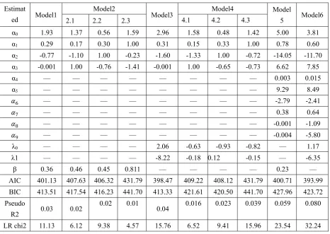
Tab 5 Estimated and statistics parameters

Estimat

ed Model1

Model2

Model3 Model4 Model

5 Model6 2.1 2.2 2.3 4.1 4.2 4.3

α0 1.93 1.37 0.56 1.59 2.96 1.58 0.48 1.42 5.00 3.81

α1 0.29 0.17 0.30 1.00 0.31 0.15 0.33 1.00 0.78 0.60

α2 -0.77 -1.10 1.00 -0.23 -1.60 -1.33 1.00 -0.72 -14.05 -11.70

α3 -0.001 1.00 -0.76 -1.41 -0.001 1.00 -0.65 -0.73 6.62 7.85

α4 — — — — — — — — 0.003 0.015

α5 — — — — — — — — 9.29 8.49

— — — — — — — — -2.79 -2.41

7 — — — — — — — — 0.38 0.64

8 — — — — — — — — -0.001 -1.09

9 — — — — — — — — -0.004 -5.80

λ0 — — — — 2.06 -0.63 -0.93 -0.82 — 1.17

λ1 — — — — -8.22 -0.18 0.12 -0.15 — -6.35

β 0.36 0.46 0.45 0.811 — — — — 0.23 — AIC 401.13 407.63 406.32 431.79 398.47 409.22 408.12 431.79 400.71 393.99 BIC 413.51 417.54 416.23 441.70 413.33 421.61 420.50 441.70 427.96 423.72 Pseudo

R2 0.03 0.02

0.02 0.01

0.04 0.016 0.023 0.039 0.059 0.080

LR chi2 11.13 6.12 9.38 4.57 15.76 6.52 9.41 15.96 23.54 32.24

directly. For the models with three parameters, model 6 is better than model 5. By contrast,

we found that the Pseudo R-2 of model 6 is larger than those of model 1 and model 3,

indicating that model 6 is much better than model 1 and model 3 with regard to goodness of

fit.

Based on the above analysis, we determined model 6 as CPM and expressed it as

follows:

N=

The excessive dispersion coefficient is:

=e

_,

where

N

— the estimate of crash amount for every year of the basic segment;

—the basic segment of the annual average daily traffic;

—the length of the basic segment; and

—the radius of the basic segment.

5.3 Prediction analysis with real data

To demonstrate the effectiveness of the prediction, we performed prediction of a certain freeway with model 1, model 3, and model 6. Then, we compared the results with the real crash data we collected from the institutions. The results are shown in Table 6.

Tab. 6 the statistics value predicted and real crashes

Obs (the sample number)

Mean Std. Dev Min Max

The real crashes 88 3.31 2.87 0 15 Prediction result of

model1

88 3.30 1.11 2.38 7.39

Prediction result of model 2

88 3.60 1.44 10.73 10.73

Prediction result of model 3

Based on the statistics of predictive value, we found that generally, the three predictive averages of the models are close to the actual casualties. When the standard deviation was used as reference, which is the description of a measurement standard of the dispersion degree of data distribution, the result of model 6 is much closer to the statistics value of the real cash data than those of the other two models. For the maximum and minimum values, the forecast range of model 6 is very close to the actual situation. Based on the above discussion, model 6 is the best among the six models.

6. Conclusion

The analysis sheds light on crash prediction of SHCS of a freeway. The influence among the different explanatory variables of the freeway traffic crash has been analyzed by super logarithmic production function. Six kinds of models from a total of 10 models were compared using AIC, BIC, and Pseudo R2 rules. Among the models, model 6, in which the interactive influence was considered, is much better than other models. Through the detailed analysis and study, the following conclusions have been drawn.

(1) With sufficient samples and data, the effective use of the GNB model in analyzing the interactive influence of explanatory variables and predicting freeway basic segments can be demonstrated.

(2) When T is selected as the excessive dispersion coefficient parameter, the AIC, BIC, and the Pseudo-R-2 values of the models tend to be small,

which indicates that the fitting effect of the

model that uses the parameter is the better than those of the others.

(3) When the interactive influence is taken into consideration, the fitting goodness of crash prediction is much better when the traffic volume, highway horizontal radius, and curve length are used.

(4) Further, prediction results with relatively good models (model 1, model 3, and model 6) have been compared to that of real data.

In summary, sufficient samples have been surveyed to establish the CMF of SHCS. Thus, the result is reliable, as proven by an example.

However, further efforts should be made to demonstrate the differences between the NB and GNB models. The experimental data were limited; thus, the model fitting effect is slightly far from ideal. Nevertheless, the influence of highway traffic crashes is universal; thus, this article adds new ideas. Furthermore, this model offers a certain reference value for crash prediction in general.

Acknowledgements

This research was supported by the National Natural Science Foundation of China (No.51408229, No. 51308059, No.51278202, No.51378222), China Postdoctoral Science Foundation（2014M552399）, Guangdong Communication Department (2013-02-068, 2015-02-003,2015-02-004), and Student Research Project of South China University of Technology (SRP:5828,7337).

Author Contributions: The experimental work, data processing and model development in this study were by Yanjie Zeng , Lineng Liu and Caifeng Jiang under the direction and supervision of Xiaofei Wang and Xinwei Li, and is based upon earlier work originally carried out by Xiaofei Wang and Xinwei Li. Yanjie Zeng and Xiaofei Wang wrote the paper.

Conflicts of Interest: The authors declare no conflict of interest.

References:

[1] Durduran S. Savas. A decision making system to automatic recognize of traffic accidents on the basis of

a GIS platform. Expert Systems with Applications.2010, 37(12): 7729-7736.

[2] White, Jules, et al. “WreckWatch: Automatic Traffic Accident Detection and Notification with

Smartphones.” Mobile Networks and Applications.2011, 16(3): 285-303.

[3] Zhong, Lian De, et al. “Accident Prediction Model of Freeway.” Journal of Beijing University of

Technology .2009,Vol.35(7):966-971.

[4] Ma Zhuang-lin, et al. Temporal-spatial Analysis Model of Traffic Accident and its Prevention Method on

Expressway. Beijing: Journal of Traffic and Transportation Engineering. 2012, Vol. 12(2).

[5] Tang Chengcheng. “Study on Key Technologies of Accident Prediction and Prevention for Two-lane

Highways [Doctor Dissertation].”Shanghai, China: Tongji University. 2009. (In Chinese)

[6] Yannis G, et al. “Driver age and vehicle engine size effects on fault and severity in young motorcyclists

accidents.” Accident Analysis and Prevention. 2005, Vol.37:327~333.

[7] Hill, J.D., and L.N. Boyle. Assessing the relative risk of severe injury in automotive crashes for older

[8] Dominique Lord. Modeling motor vehicle crashes using Poisson-gamma models: examining the effects

of low sample mean values and small sample size on the estimation of the fixed dispersion parameter.

Accident Analysis and Prevention. 2006, Vol.38:751~766.

[9] Liu, Bor Shong. Association of intersection approach speed with driver characteristics,vehicle type and

traffic conditions comparing urban and suburban areas. Accident Analysis and Prevention.

2007,Vol.39(2):216~223.

[10] N.N Sze,., and S.C. Wong. Diagnostic analysis of the logistic model for pedestrian injury severity in traffic

crashes. Accident Analysis and Prevention. 2007, Vol.39: 1267~1278.

[11] Rhodes, Nancy, and K. Pivik. Age and gender differences in risky driving: the roles of positive affect and

risk perception. Accident Analysis and Prevention.2011, Vol. 43 (3):923~931.

[12] Organization for Economic Co-operation and Development Scientific Expert Group. Road Safety

Principles and Models: Review of Descriptive, Predictive, Risk and Accident Consequence Models. Paris:

Crashes, 1997:105.

[13] Miaou, S.P., H. Lum. Modeling vehicle accident and highway geometric design relationships. Accidents

Analysis and Prevention. 1993, Vol.25 (6):42~51.

[14] Fridstrøm, Lasse, et al. Measuring the contribution of randomness, exposure, weather and daylight to

the variation in road accident counts. Accident Analysis and Prevention. 1995,Vol.27 (1): 1–20.

[15] Bozdogan, Hamparsum. Model selection and Akaike’s information criterion (AIC): the general theory and

its analytical extensions. Psychometrika. 1987, Vol. 52 (3):345~370.

[16] Christensen, L.R., D.W. Jorgenson, and L.J Lau. Transcendental logarithmic production frontiers. Review

of Economics & Statistics.1973,Vol. 55 (1):28~45.

[17] Huang, Wei. Scope Economy of China’s Insurance Industry—Based on the Generalized Translog Cost

Function. The Journal of Quantitative & Technical Economics.2007, Vol.11:86~95

[18] Li，Li, Yaoming Wu, and Liu Yang. The Application of Generalized Translog Cost Function in Scale

Economy Analysis. Statistics & Decision.2011, Vol.20: 173~176

[19] António Couto, , and Sara Ferreira. A note on modeling road accident frequency: A flexible elasticity

model. Accident Analysis and Prevention . 2011, Vol.43:2104~2111.

[20] Wu, Lurong, Fangfang Liang, and Zhikai Shi. " The Translog Production Function model of the traffic

accident loss in China." Mathematics in Practice andTheory.2010,Vol.40(22):56~61

[21] Zeng, Juan. “Research on Influencing Factors of Socio-economic Losses of Road Traffic Accident Based

on Generalized Linear Models.” Journal of Wuhan University of Technology.2010,Vol.32(6): 155~158

[22] Li, Rong，Xiang Liu, and Jian Liu.Research on Traffic Accident Frequency Prediction Based on Translog

Production Function. Journal of Hunan University(Natural Sciences).2013,Vol.40(4):49~54

[23] Liu, Xiang. Research of Road Safety Based on Human and Environment Factors [Master Dissertation].

[24] Hauer, E., and J. Bamfo. Two tools for finding what function links the dependent variable to the

explanatory variables. In: Proceedings of the ICTCT Conference, Lund. 1997.