Volume 8, No. 5, May-June 2017
International Journal of Advanced Research in Computer Science RESEARCH PAPER
Available Online at www.ijarcs.info
ISSN No. 0976-5697
Comprehensive Evaluation and Interpretation of PCAon Multiple Datasets
Rabia Nazir
StudentM. Tech, Dept. of Computer Sc& IT, Univ. of Jammu, J&K , India
Abid Sarwar
Assistant Professor Dept. of Computer Sc& IT Univ. of Jammu, J&K, IndiaAmit Sharma
Assistant Professor Dept. of Computer Sc& IT Univ. of Jammu, J&K, IndiaVinod Sharma
ProfessorDept. of Computer Sc& IT University of Jammu, India
Abstract: Principal component analysis is a statistical based technique that reduces the data size and preserves most of the variance in the form of new variables called principal components. In this paper, MATLAB is used to evaluate and analyze PCA on multiple datasets collected from multiple data sources. PCA reduces the size of the datasets by at least 68% without any loss of significant information and the effectiveness of reduced datasets is increased.
Keywords: PCA; Dimensionality Reduction; Feature Extraction; Eigenvalues; Principal components.
1. INTRODUCTION
The era we are living in is an era of Digital Universe where the size of data is doubled every two years. The rapid increase in complexity and volume of data is a major problem for data analysis [Cheng, You (2016)]. This is due to the imprecation of dimensionality. Dimensionality reduction is an efficacious approach to reduce the data size. It is process of reducing the number of arbitrary variables or attributes under consideration [Snehal K., Machchhar (2014)]. It obtains reduced representation of data set that is much more minuscule in size but generates virtually the same analytical results. It is used to solve machine learning problems in order to obtain better features for a classification or regression task. It is a data preprocessing step used to reduce data size for analysis. It is different from compression in a way that compression reconstructs the exact original data while dimensionality reduction reconstructs data that is similar to the original data. Two main approaches under dimensionality reduction are feature selection and feature extraction [Varghese et al. (2012)]. Feature selection approaches endeavor to find a subset of the primary variables. Feature selection is a technique which is utilized to find the good quality of relevant features from the initial dataset utilizing some objective measures [Kumar, Elavarasan (2014)]. Main purposes of feature selection are- it makes training efficient and it removes noise feature that otherwise tends to increase classification error on new data. Three basic methods of feature selection are filter method, wrapper method and embedded method.
Feature extraction approach obtains the most relevant information from original dataset by reducing the number of resources that are required to represent the original dataset. Combinations of the variables are used to solve problems while still retaining the information with sufficient accuracy. Two basic methods of feature extraction are principal component analysis and linear discriminant analysis.
2. LITERATURE REVIEW
The most widely used techniques in face recognition PCA and LDA are discussed. These two techniques are explained and their merits and demerits are used to compare these two techniques. The differences between PCA and LDA are highlighted. Analyzing the performance of both techniques on images, it is concluded that PCA performs better as compared to LDA [Kaur et al. (2014)].
Face recognition is performed using PCA and LDA. Results show that LDA has greater accuracy than the accuracy of PCA when sample size is high. For both algorithms same databases are used i.e, ORL and UMIST. Images of ORL database are front viewed and the images obtained from UMIST database are side viewed. Quick comparison between test images and learned training images are performed by PCA and thus, eigenfaces are used as compact storage. For UMIST database PCA shows 88.33% accuracy and LDA has 91.11% accuracy. For ORL database, PCA has 96.11% and LDA has 98.22% accuracy [Mahmud et al. (2015)].
A general overview of PCA is presented along with its advantages and applications. Staring with the importance of PCA in biometrics, features and importance of PCA in face recognition are highlighted. The algorithm of PCA is discussed along with its advantages and disadvantages. Since PCA is unsupervised technique it is more suitable for databases with no class labels. Detailed description of PCA utilized in face recognition is presented [Karamizadehet al.
(2013)].
A hybrid approach of PCA and DCT is proposed for face recognition. This hybrid method is used to improve the recognition rate of face recognition system. FACES94 and ORL are the standard databases used to analyze experimental results and it is observed that the proposed hybrid system achieves more accurate results. DCT is used as a preprocessing step and then features are extracted using PCA. DCT is used to eliminate redundancies and extract most significant elements from an image and PCA expresses every image by operating linearly on eigenvectors [Kadam (2014)].
Principal component analysis is evaluated in presence of missing values and it was found that principal component analysis can be suitable for most of the practical datasets. If the observations are sparse and the missing values are to be reconstructed using the available data, a probabilistic formulation of PCA is used. The correlation between variables is captured to reconstruct the missing values. Experiments are conducted on Netflix data. PCA is considered as one of the most popular techniques by Netflix contestants [Ilin ,Raiko (2010)].
3 MATERIAL AND METHODS
3.1 Datasets
Principal component analysis is applied on four datasets using MATLAB 2013a. The description about the datasets is given below.
3.1.1 Breast cancer Wisconsin (diagnostic) data set: Features from the digitized image of breast mass are computed. The fine needle aspirate (FNA) of a breast mass describes the characteristics of the cell nuclei present in the image.
Attribute Information- First is ID number and 2-31 are ten real valued features computed for nucleus of every cell. The ten features are radius, texture, perimeter, area, smoothness, compactness, concavity, concave points, and symmetry and fractal dimension. This dataset is available at kaggle.com. 3.1.2 Credit card fraud detection:
The dataset contains information about transactions made by European cardholders on September 2013 using credit cards. Transactions of only two days are present in the dataset and it consists of 492 frauds out of 284,807 total transactions. A research collaboration of Worldline and the Machine Learning Group of UniversiteLibre de Bruxelles collected and analyzed the data on big data mining and fraud detection. The data is available at kaggle.com.
3.1.3 Face dataset:
Image is a collection of pixels and each pixel contains information of its position and intensity. Using the pixel information of each pixel the data is stored in numeric form. The dataset consists of pixel level image of faces of various persons. Input is 48 × 48 pixel gray level values between 0- 255. The dataset consists of 4178 images and each image has 2304 attributes. The data is available at inclass.kaggle.com.
3.1.4 Smear dataset:
Data is used from the thesis of Byriel (1999). It is a dataset of pictures of pap smear cells of uterine cervix. Features are extracted from the pictures by segmenting the images and then analyzing the original and segmented images. Measurements of each feature of the cells are stored in tabular form. The features are nucleus area, nucleus
brightness, nucleus longest diameter, cytoplasm shortest diameter, cytoplasm roundness, nucleus relative position, maxima in cytoplasm, cytoplasm area, cytoplasm brightness, nucleus elongation, cytoplasm longest diameter, nucleus perimeter, maxima in nucleus, maxima in cytoplasm, nucleus to cytoplasm ratio, nucleus roundness, cytoplasm elongation, cytoplasm perimeter and minima in nucleus. This dataset is available at http://mde-lab.aegean.gr.
3.2 Algorithm (PCA)
Principal component analysis is a data reduction technique, developed by Karl Pearson in 1901 and then later on independently developed and named by H.Hotelling in 1933. Data size is reduced in such a way that most of the variation of original data is retained [Nick et al. (2015)]. Principal component analysis is a statistical based approach in which orthogonal transformations are used to convert a set of observations that may be correlated into a set of variables that are linearly uncorrelated [Elavarasan, Mani (2015)]. These set of new variables are called as principal components and the number of principal components may be less or equal to the number of original variables. This transformation is based on the variance of the data and the first principal component always represents the highest variance [Paul et al. (2013)]. Principal component analysis is used in various areas like Image Compression, Biometrics, Face Recognition, Protein Classification etc. [Ramadevi ,Usharani (2013)].
4 METHODOLOGY
The following steps are involved in principal component analysis.
I. Get data and normalize it
We can take any dataset and in the first step we have to normalize it. I have taken a dataset of faces where row vector represents various images and column vector contains pixel values of images. First we have to calculate mean of the dataset and then subtract the mean value from each value of the dataset.
𝜇𝜇=�1𝑛𝑛� � 𝑥𝑥𝑖𝑖 𝑛𝑛
𝑖𝑖=1
Where X is a vector containing all values of the dataset and n is the number of values in the whole dataset.
𝑋𝑋𝑁𝑁=𝑋𝑋 − 𝜇𝜇
Where 𝑋𝑋𝑁𝑁 is the normalized vector and X is original vector. The normalized vector has zero mean value. It centralizes the data and thus simplifies computation.
II. Calculate covariance matrix
Covariance is a measure of joint variability of two variables. Variance is measure of spread of data in a dataset. These two terms are same but variance is for one dimensional data and covariance is measured between two dimensions.
𝐶𝐶=∑𝑛𝑛𝑖𝑖=1𝑛𝑛 −𝑋𝑋𝑁𝑁1𝑋𝑋𝑁𝑁𝑇𝑇
An eigenvector is a vector on which when we apply any operator it gives scalar multiple of itself. Eigenvectors give us information about the patterns in data. Let e be a vector and C be the matrix. Multiplying matrix by the vector, then𝐶𝐶𝐶𝐶 is the new vector. 𝐶𝐶𝐶𝐶is just e multiplied by a number
𝜆𝜆. Therefore,
𝐶𝐶𝐶𝐶= 𝜆𝜆𝐶𝐶
is the equation that has to be solved to get eigenvectors and eigenvalues.
IV. Construct a feature vector
Arrange all the eigenvalue in non-increasing order. The eigenvectors with highest eigenvalues contain most of the information, thus, we can ignore eigenvectors with lower eigenvalues. By arranging eigenvectors we get components in order of significance. Now we can ignore eigenvectors with lesser significance. By leaving out some components the final dataset will have less number of dimensions. Take
𝐾𝐾 number of highest eigenvectors and place in a matrix. This matrix is feature vector.
V. Derive new variables
Take transpose of both feature vector and normalized dataset. Feature vector is transposed so that eigenvectors are represented by rows with most significant eigenvectors at the top. Normalized dataset is transposed so that each row holds a separate dimension. The final dataset that is obtained in this step contains data items in columns and dimensions in rows. Now we represent data in terms of eigenvectors or principal components.
𝐹𝐹𝑖𝑖𝑛𝑛𝐹𝐹𝐹𝐹𝐹𝐹𝐹𝐹𝐹𝐹𝐹𝐹= (𝐹𝐹𝐶𝐶𝐹𝐹𝐹𝐹𝐹𝐹𝐹𝐹𝐶𝐶𝐹𝐹𝐶𝐶𝐹𝐹𝐹𝐹𝐹𝐹𝐹𝐹)𝑇𝑇× (𝑋𝑋 𝑁𝑁)𝑇𝑇
VI. Recover original data
Take inverse of transposed feature vector and multiply it with the final dataset that was calculated in previous step. Then add mean value to the result.
𝑅𝑅𝐶𝐶𝐹𝐹𝐹𝐹𝐹𝐹𝐶𝐶𝐹𝐹𝐶𝐶𝑅𝑅𝐹𝐹𝐹𝐹𝐹𝐹𝐹𝐹
= (𝐹𝐹𝐶𝐶𝐹𝐹𝐹𝐹𝐹𝐹𝐹𝐹𝐶𝐶vector−1×𝐹𝐹𝑖𝑖𝑛𝑛𝐹𝐹𝐹𝐹𝐹𝐹𝐹𝐹𝐹𝐹𝐹𝐹) + 𝜇𝜇
5 EXPERIMENTAL RESULTS
The datasets are stored in Microsoft excel file with .xls or .xlsx extension. To use the dataset in MATLAB we convert the files to .mat format. Then the datasets are loaded into MATLAB and PCA is performed.
The first dataset is breast cancer dataset with 570 instances and each instance consists of 31 attributes. Number of features or principal components selected for dimensionality reduction depends on the variance of data. While selecting the number of principal components, the maximum variance of the data should be retained. We select first 7 components retaining 90% of the variance. After applying PCA we plot the original normalized data and the recovered data. We chose an instance of the dataset randomly and plot its original and recovered attributes separately.
[image:3.595.318.561.56.283.2]Analyzing the scatter plot (Fig. 1.) of original and recovered data, there is not much difference. Only the scaling factor varies. Thus PCA reduced the size of dataset by 70% while retaining the information needed.
Fig. 1. Output of breast cancer dataset.
The second dataset is credit card fraud detection consisting of 250 instances and each instance has 31 attributes. In this dataset only 5 principal components are selected. A random instance of the data is selected to plot the original and recovered data. Recovered data is the data that is recovered from the principal components.
Fig. 2. Output of credit card fraud detection dataset.
It is evident from the scatter plots (Fig. 2.) that there is no visible difference between the two. Thus PCA reduces the size of the dataset by approx. 83% without loss of any valuable information.
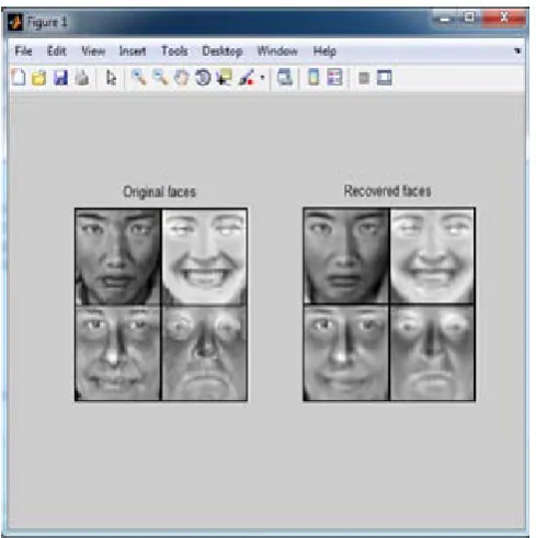
[image:3.595.318.556.395.626.2]principal components to represent the whole data can be changed to analyze the effect on recovered images.
Fig. 3. Output of face dataset with number of eigenvectors = 90.
Fig. 4. Output of face dataset with number of eigenvectors = 300.
The number of eigenvectors chosen to represent the dataset depends on the quality of images we want to recover. After analyzing the results by varying the number of eigenvectors(𝐾𝐾) it was observed that
• At 𝐾𝐾= 90 (Fig. 3.), the recovered images are blur and the images cannot be identified properly.
• At 𝐾𝐾= 300 (Fig. 4.), the recovered images are less blur and the images can be identified.
• At 𝐾𝐾= 800(Fig. 5.), the recovered images are better.
[image:4.595.318.572.113.354.2]• Further increasing the value of 𝐾𝐾 has no significant effect on the images.
Fig. 6. Output of face dataset with number of eigenvectors = 800.
Next dataset is cervical cancer dataset. It consists of various features of pap smear cells of uterine cervix. The dataset contains 454 instances and each instance has 25 features. 8 Eigen vectors or principal components are selected. A random instance of the data is selected to plot the original and recovered data. Recovered data is the data that is recovered from the principal components.Reducing the size of dataset by almost 68%, PCA retains the important information.
[image:4.595.39.284.372.618.2] [image:4.595.318.562.524.731.2]6 CONCLUSION
Dimension reduction was brought in to overcome the problem of dimensionality when dealing with high dimensional data. Principal component analysis is used as a tool for reducing the number of variables in the original dataset to a smaller number of variables that capture most of the variance of original dataset. All attributes used to represent data do not contain valuable information and thus least significant attributes can be ignored. Various datasets have been used and it is observed that PCA is an effective technique of reducing the dimension without losing any substantial information.
7 FUTURE SCOPE
In future, principal component analysis can be applied to various other image processing algorithms in different domains. Also, PCA could be implemented on tools other than MATLAB. Some other datasets can be also studied. PCA can be compared to other dimensionality reduction techniques.
REFERENCES
1. BoradeSushmaNiket; Dr. Adgaonkar Ramesh P. (2011); Comparative analysis of PCA and LDA. ICBEIA.
2. Cheng Long; You Cheny (2016): Hybrid Non-Linear Dimensionality Reduction Method Framework Based on Random Projections, IEEE International Conference on Cloud Computing and Big Data Analysis.
3. Elavarasan N.; Dr. Mani K. (2015): A Survey on Feature Extraction Techniques ,IJIRCCE, Vol. 3, Issue 1.
4. Ilin Alexander; RaikoTapani (2010): Practical Approaches to Principal Component Analysis in the Presence of Missing Values, JMLR 11.
5. Kadam Kiran D. (2014): Face Recognition using Principal Component Analysis with DCT. IJERGS, Volume 2, Issue 4. 6. KaramizadehSasan; Abdullah Shahidan M.; ManafAzizah
A.; ZamaniMazdak; HoomanAlireza (2013): An Overview of Principal Component Analysis. SCIRP, 4,pp. 173-175. 7. Kaur Amritpal; Singh Sarabjit; Taqdir (2015): Face
recognition using PCA and LDA techniques, IJARCCE, Vol. 4, Issue 3.
8. Kumar V. Arul; Elavarasan N. (2014): A Survey on Dimensionality Reduction Technique. IJETTCS, Volume 3, Issue 6.
9. Mahmud Firoz; TaskiaKhatunMst.; TauhidZuhori Syed; Afroge Shyla; Aktar Mumu; pal Biprodip (2015): Face recognition using principal component analysis and linear discriminant anlysis”, 2nd Int'l Conf. ICEEICT Jahangirnagar University, Dhaka, Bangladesh.
10. Nick William; Shelton Joseph; Bullock Gina; Esterline Albert; AsameneKassahun (2015): Comparing Dimensionality Reduction Techniques, Proceedings of the IEEE Southeast Con 2015, Florida.
11. Paul Linton Chandra; Al Saman Abdulla; Sultan Nahid: Methodological Analysis of Principal Component Analysis (PCA) Method. IJCEM, Vol. 16 Issue 2.
12. Ramadevi G. N.; Usharani K. (2013): Study on Dimensionality Reduction Techniques and Applications. IJPAPER, Vol 04, Special Issue01.
13. Snehal K Joshi.; MachchharSahista (2014): An Evolution and Evaluation of Dimensionality Reduction Techniques- A Comparative Study. IEEE International Conference on Computational Intelligence and Computing Research. 14. Varghese Nebu; Verghese Vinay; Prof. P. Gayathri and Dr.