www.ijiset.com
Solving Aggregate Planning Problem Using LINGO
Anand Jayakumar AP
1
P
, Krishnaraj CP
2
P
and Balakrishnan SP
3
P
1
P
Department of Mechanical Engneering, SVS College of Engineering, Coimbatore, Tamil Nadu, India
P
2
P
Department of Mechanical Engneering, Karpagam College of Engineering, Coimbatore, Tamil Nadu, India
P
3
P
Department of Mechanical Engneering, United Institute of Technology, Coimbatore, Tamil Nadu, India
Abstract
The goal of aggregate planning is to maximize profit while meeting demand. Aggregate planning is an operational activity that does an aggregate plan for the production process, in advance of 6 to 18 months, to give an idea to management as to what quantity of materials and other resources are to be procured and when, so that the total cost of operations of the organization is kept to the minimum over that period. In this paper we solve a numerical problem using LINGO software.
Keywords: 25TAggregate planning; Maximize profit; LINGO.
1. Introduction
The goal of aggregate planning is to maximize profit while meeting demand. Every company, in its effort to meet customer demand, faces certain constraints, such as the capacity of its facilities or a supplier’s ability to deliver a component. A highly effective tool for a company to use when it tries to maximize profits while being subjected to a series of constraints is linear programming. Linear programming finds the solution that creates the highest profit while satisfying the constraints that the company faces.
2. Literature Review
Ghulam Asghar et al (1), have made a study about the suggestion of an alternate model of medium range/aggregate production planning (APP) for the process industry. This research is conducted according to the forecasted demand of six months of a leading Cement Industry of Pakistan. Different alternatives have been discussed and a proposed model has been developed and analyzed.
Seema Sarkar (Mondal) and Savita Pathak (2) have presented an application of fuzzy mathematical programming model to solve aggregate production
planning (APP). Fuzzy logic was applied to solve the uncertain production, demand, capital and warehouse spaces. All costs are taken as triangular fuzzy numbers. Model is developed such that the system takes minimum subcontracted units in each period and no inventories at the end of the planning horizon
Mohamed K. Omar et al (3) have developed a a fuzzy mixed-integer linear programming (FMILP) modeling approach to deal with the multi-product APP problems confronting the specialty chemical plant. The objective of the proposed model is to minimize the sum of production, set-up, inventory, backorder and workforce costs. The model formulation incorporates the fuzzy set theory and possibilistic theory to define the uncertainties that appear in the model’s objective and constraints.
Navid Mortezaei et al (4), develop a new multi-objective linear programming model for general APP for multi-period and multi-product problems. They have assumed that, there is uncertainty in critical input data (i.e., market demands and unit costs). This model is suitable for 24-hour production systems. To show practicality of their model, they have implemented this model in a case study.
MstNazma Sultana et al (5), have discussed aggregate planning strategies and a special structure of transportation model is investigated for the aggregate planning purpose of ―Bangladesh Cable Shilpa Ltd, Khulna‖. For this transportation problem, all the unit costs, supplies, demands & other values are taken from a case study. The forecasting demand values are determined using Single Exponential Smoothing Forecasting technique. A real life unbalanced transportation problem is discussed and solved to bring the most efficient technique of reducing transportation and storage cost.
www.ijiset.com
generalized model of single-item resource constrained aggregate production planning (APP) with linear cost functions. In this paper, They have developed the proposed genetic algorithm with effective operators for solving the proposed model with an integer representation. This model is optimally solved and validated in small-sized problems by an optimization software package, in which the obtained results are compared with GA results. The results imply the efficiency of the proposed GA achieving to near optimal solutions within a reasonably computational time.
Mansoureh Farzam Rad and Hadi Shirouyehzad (7), have suggested an aggregate production planning model for products of Hafez tile factory during one year. Due to this fact that the director of the company seeks 3 main objectives to determine the optimal production rate, the linear goal planning method was employed. After solving the problem, in order to examine the efficiency and the distinctiveness of this method in compare to linear programming, the problem was modeled just by considering one objective then was solved by linear programming approach. The findings revealed the goal programming with multi objectives resulted more appropriate solution rather than linear programming with just one objective.
Reza Ramezanian et al (8), have presented a paper on multi-period, multi-product and multi-machine systems with setup decisions. In this study, they developed a mixed integer linear programming (MILP) model for general two-phase aggregate production planning systems. Due to NP-hard class of APP, they implement a genetic algorithm and tabu search for solving this problem. The computational results show that these proposed algorithms obtain good quality solutions for APP and could be efficient for large scale problems.
Carlos Gomes da Silvaa et al (9), have presented an aggregate production planning (APP) model applied to a Portuguese firm that produces construction materials. A multiple criteria mixed integer linear programming (MCMILP) model is developed with the following performance criteria: (1) maximize profit, (2) minimize late orders, and (3) minimize work force level changes. It includes certain operational features such as partial inflexibilityof the work force, legal restrictions on workload, work force size (workers to be hired and downsized), workers in training, and production and inventory capacity . The purpose is to determine the number of workers for each worker type, the number of overtime hours, the inventory level for each product category, and the level of subcontracting in order to meet the forecasted demand for a planning period of 12 months.
Mohammed. Mekidiche et al (10), have presented a new formulation of Weighted Additive fuzzy goal programming model. The proposed formulation attempts to minimize total production and work force costs, carrying inventory costs and rates of changes in Work force. A real-world industrial case study demonstrates applicability of proposed model to practical APP decision problems. LINGO computer package has been used to solve final crisp linear programming problem package and getting optimal production plan.
Simon Chinguwa et al (11), have made a study that investigates the best model of aggregate planning activity in an industrial firm and uses the trial and error method on spreadsheets to solve aggregate production planning problems. Also linear programming model is introduced to optimize the aggregate production planning problem. Application of the models in a furniture production company is evaluated to demonstrate that practical and beneficial solutions can be obtained from the models. Finally some benchmarking of other furniture manufacturing industries was undertaken to assess
relevance and level of use in other furniture firms.
F. Khoshalhan and A. Cheraghali Khani (12), have proposed an integrated aggregate production planning model considering the time and costs of maintenance. This model indicates the optimum production size among the optimum time of preventive maintenance. As a final point, in order to check the reliability of the proposed model, an example has been examined. Results show that a considerable amount of cost has been saved by applying the model.
3. The Problem
We illustrate linear programming through the discussion of Red Tomato Tools, a small manufacturer of gardening equipment with manufacturing facilities in Mexico. Red Tomato’s products are sold through retailers in the United States. Red Tomato’s operations consist of the assembly of purchased parts into a multipurpose gardening tool. Because of the limited equipment and space required for its assembly operations, Red Tomato’s capacity is determined mainly by the size of its workforce.
For this example we use a six-month time period because this is long enough time horizon to illustrate many of the main points of aggregate planning.
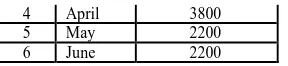
Table 1: Demand Forecast at Red Tomato Tools S.No Month Demand Forecast
www.ijiset.com
4 April 3800
5 May 2200
6 June 2200
The demand for Red Tomato’s gardening tools from consumers is highly seasonal, peaking in the spring as people plant their gardens. This seasonal demand ripples up the supply chain from the retailer to Red Tomato, the manufacturer. Red Tomato has decided to use aggregate planning to overcome the obstacle of seasonal demand and maximize profits. The options Red Tomato has for handing the seasonality are adding workers during the peak season, subcontracting out some of the work, building up inventory during the slow months, or building up a backlog of orders that will be delivered late to the customers. To determine how to best use these options through an aggregate plan, Red Tomato’s vice president of supply chain starts with the first task – building a demand forecast. Although Red Tomato could attempt to forecast this demand itself, a much more accurate forecast comes from a collaborative process used by both Red Tomato and its retailers to produce the forecast shown in Table 1.
Red Tomato sells each tool to the retailers for $40. The company has a starting inventory in January of 1000 tools. At the beginning of January the company has a workforce of 80 employees. The plant has a total of 20 working days in each month and each employee earns $4 per hour regular time. Each employee works eight hours per day on straight time and the rest on overtime. As discussed previously, the capacity of the production operation is determined primarily by the total labor hours worked. Therefore, machine capacity does not limit the capacity of the production operation. Because of labor rules, no employee works more than 10 hours overtime per month. The various costs are shown in Table 2.
Table 2: Demand Forecast at Red Tomato Tools
S.No Item Cost
1 Material cost $10/unit 2 Inventory holding cost $2/unit/month 3 Marginal cost of stockout/ $5/unit/month
backlog
4 Hiring and training costs $300/worker 5 Layoff cost $500/worker 6 Labor hours required 4/unit 7 Regular time cost $4/hour 8 Overtime cost $6/hour 9 Cost of subcontracting $30/unit
Currently, Red Tomato has no limits on subcontracting, inventories and stockouts /backlog. All stockouts are backlogged and supplied from the following month’s production. Inventory costs are incurred on the ending inventory in the month. The supply chain manager’s goal is to obtain the optimal aggregate plan that allows Red Tomato to end June with at least 500 units (ie, no
stockouts at the end of June and at least 500 units in inventory).
The optimal aggregate plan is one that results in the highest profit over the six month planning horizon. For now, given Red Tomato’s desire for a very high level of customer service, assume all demand is to be met, although it can be met late. Therefore the revenues earned over the planning horizon are fixed. As a result, minimizing cost over the planning horizon is the same as maximizing profit. In many instances, a company has the option of not meeting certain demand, or price itself may be a variable that a company has to determine based on the aggregate plan. In such a scenario, minimizing cost is not equivalent to maximizing profits.
4. The Modeling Framework
Decision Variables
The first step in constructing an aggregate planning model is to identify the set of decision variables whose values are to be determined as part of the aggregate plan.
WRtR = workforce size for month t, t = 1…..6 HRtR = number of employees hired at the beginning of Month t, t = 1…..6
LRtR = number of employees laid off at the beginning of Month t, t = 1…..6
PRtR = number of units produced in Month t, t….6 IRtR = Inventory at the end of Month t, t….6 SRtR = number of units stocked out/backlogged at the end of Month t, t….6
CRtR = number of units subcontracted for Month t, t….6 ORtR = number of overtime hours worked in Month t, t….6 Objective Function
Denote the demand in Period t by DRtR. The values of DRtR are as specified by the demand forecast in Table 1. The objective function is to minimize the total cost (equivalent to maximizing total profit as all demand is to be satisfied) incurred during the planning horizon. The cost incurred has the following components:
1. Regular – time labor cost: Recall that workers are paid a regular – time wage of $640 ($4/hour x 8 hours/day x 20 days/month) per month. Because WRtR is the number of workers in period t, the regular – time labour cost over the planning horizon is given by
www.ijiset.com
worked in period t, the overtime cost over the planning horizon is
3. Cost of hiring and layoffs: The cost of hiring a worker is $300 and the cost of laying off a worker is $500. HRtR and LRtR represent the number of hired and the number laid off, respectively in Period t. Thus, the cost of hiring and layoff is given by
4. Cost of inventory and stockout: The cost of carrying inventory is $2 per unit per month and the cost of stocking out is $5 per unit per month. IRtR and SRtR represent the units in inventory and the units stocked out respectively in period t. Thus the cost of holding inventory and stocking out is
5. Cost of materials and subcontracting: The material cost is $10 per unit and the subcontracting cost is $30/unit. PRtR represents the quantity produced and CRtR represents the quantity subcontracted in period t. Thus the material and subcontracting cost is
6. Final Objective: The total cost incurred during the planning horizon is the sum of all the aforementioned costs and is given by
Red Tomato’s objective is to find an aggregate plan that minimizes the total cost incurred during the planning horizon. The values of the decision variables in the objective function
cannot be set arbitrarily. They are subjected to a variety of constraints defined by available capacity and operating policies. The next step in setting up the aggregate planning model is to define clearly the constraints linking the decision variables.
Constraints
• Workforce, hiring and layoff constraints: the
workforce size Wt in period t is obtained by adding the number hired Ht in period t to the workforce size Wt-1 in period t-1, and subtracting the number laid off Lt in Period t. The starting workforce size is given by W0 = 80.
• Capacity constraints: In each period, the amount produced cannot exceed the available capacity. This set of constraints limits the total production by the total internally available capacity (which is determined based on the available labour hours, regular or overtime). Subcontracted production is not included in this constraint because the constraint is limited to production within the plant. As each worker can produce 40 units per month on regular time (four hours per unit ) and one unit for every four hours overtime, we have the following
• Inventory balance constraints: The third set of constraints balances inventory at the end of each period. Net demand for Period t is obtained as the sum of the current demand Dt and the previous backlog S. This demand is either filled from current production (in-house production Pt, or subcontracted production Ct) and previous inventory It-1 (in which case some inventory It may be left over) or part of it is backlogged St. This relationship is captured by the following equation. The starting inventory is given by I0 = 1000, the ending inventory must be at least 500 units (i.e. I0 > 500), and initially there are no backlogs (i.e. S0 = 0).
• Overtime limit constraints: The fourth set of
constraints requires that no employee work more than 10 hours of overtime each month. This requirement limits the total amount of overtime hours available as follows. In addition, each variable must be nonnegative and there must be no backlog at the end of period 6 (i.e. S0 = 0).
5.
LINGO PROGRAM
Model:
Min = Total_cost;
www.ijiset.com
RTLC = 640 * (W1 + W2 + W3 + W4 + W5 + W6);
OLC = 6 * (O1 + O2 + O3 + O4 + O5 + O6); CHL = 300 * (H1 + H2 + H3 + H4 + H5 + H6)
+ 500 * (L1 + L2 + L3 + L4 + L5 + L6);
CIS = 2 * (I1 + I2 + I3 + I4 + I5 + I6) + 5 * (S1 + S2 + S3 + S4 + S5 + S6);
CMS = 10 * (P1 + P2 + P3 + P4 + P5 + P6)
+ 30 * (C1 + C2 + C3 + C4 + C5 + C6);
W0 = 80;
W1 = W0 + H1 - L1; W2 = W1 + H2 - L2; W3 = W2 + H3 - L3; W4 = W3 + H4 - L4; W5 = W4 + H5 - L5; W6 = W5 + H6 - L6; P1 <= 40 * W1 + O1/4; P2 <= 40 * W2 + O2/4; P3 <= 40 * W3 + O3/4; P4 <= 40 * W4 + O4/4; P5 <= 40 * W5 + O5/4; P6 <= 40 * W6 + O6/4; S0 = 0;
I0 = 1000; I6 = 500; S6 = 0; D1 = 1600; D2 = 3000; D3 = 3200; D4 = 3800; D5 = 2200; D6 = 2200;
I0 + P1 + C1 = D1 + S0 + I1 - S1; I1 + P2 + C2 = D2 + S1 + I2 - S2; I2 + P3 + C3 = D3 + S2 + I3 - S3; I3 + P4 + C4 = D4 + S3 + I4 - S4; I4 + P5 + C5 = D5 + S4 + I5 - S5; I5 + P6 + C6 = D6 + S5 + I6 - S6; O1 <= 10 * W1;
O2 <= 10 * W2; O3 <= 10 * W3; O4 <= 10 * W4; O5 <= 10 * W5; O6 <= 10 * W6;
W1 >= 0; W2 >= 0; W3 >= 0; W4 >= 0;W5 >= 0;W6 >= 0; O1 >= 0;O2 >= 0;O3 >= 0; O4 >= 0;O5 >= 0;O6 >= 0; H1 >= 0;H2 >= 0;H3 >= 0; H4 >= 0;H5 >= 0;H6 >= 0; L1 >= 0;L2 >= 0;L3 >= 0; L4 >= 0;L5 >= 0;L6 >= 0; I1 >= 0;I2 >= 0;I3 >= 0;
I4 >= 0;I5 >= 0;I6 >= 0; S1 >= 0;S2 >= 0;S3 >= 0; S4 >= 0;S5 >= 0;S6 >= 0; P1 >= 0;P2 >= 0;P3 >= 0; P4 >= 0;P5 >= 0;P6 >= 0; C1 >= 0;C2 >= 0;C3 >= 0; C4 >= 0;C5 >= 0;C6 >= 0;
@GIN(W1);@GIN(W2);@GIN(W3);
@GIN(W4);@GIN(W5);@GIN(W6);
@GIN(H1);@GIN(H2);@GIN(H3);
@GIN(H4);@GIN(H5);@GIN(H6);
@GIN(L1);@GIN(L2);@GIN(L3);
@GIN(L4);@GIN(L5);@GIN(L6);
@GIN(I1);@GIN(I2);@GIN(I3);
@GIN(I4);@GIN(I5);@GIN(I6);
@GIN(S1);@GIN(S2);@GIN(S3);
@GIN(S4);@GIN(S5);@GIN(S6);
@GIN(P1);@GIN(P2);@GIN(P3);
@GIN(P4);@GIN(P5);@GIN(P6);
@GIN(C1);@GIN(C2);@GIN(C3);
@GIN(C4);@GIN(C5);@GIN(C6);
End
6.
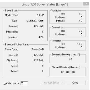
Computational Efficiency
An intel CORE i5 processor (Second Generation) with 4GB RAM was used to process the model. Windows 7 was the operating system. Branch and Bound solver was used.
A. Numerical Problem size
Total variables: 52 Nonlinear variables: 0 Integer variables: 40 Total constraints: 79 Nonlinear constraints: 0 Total nonzeros: 189 B. Run Time
The problem was solved in less than 1 second.
www.ijiset.com
7.
Result
By optimizing the objective function subjected to listed constraints the aggregate plan is shown in table 3 and 4.
TABLE 3: Aggregate Plan – Part I
TABLE 4: Aggregate Plan – Part II
Total cost over the planning horizon is $422660. Red Tomato lays off a total of 16 employees at the beginning of January. After that the company maintains the workforce and production level. They use the subcontractor during the month of April. They carry a backlog only from April to May. In all other months, they plan no stockouts. In fact Red Tomato carries inventory in all other periods. We describe this inventory as seasonal inventory because it is carried in anticipation of a future increase in demand. Given the sale price of $40 per unit and total sales of 16000 units revenue over the planning horizon is $640000.
8. Conclusion
Thus the global optimal solution was found. Thus in this paper we have used LINGO program to solve the SCND problem. The answer is the same as obtained using excel solver by Sunil Chopra et al (13). The LINGO program is much faster. All optimization problems can be solved by using LINGO.
References
[1] Ghulam Asghar, Wasif Safeen, Mirza Jahanzaib, ―An alternate model of aggregate production planning for process industry: a case of cement plant‖, Technical Journal, Vol. 20(SI) No II (S) , 2015, pp 12 – 18.
[2] Seema Sarkar (Mondal) and Savita Pathak , ―Possibilistic
linear programming approach to the multi item aggregate
production planning‖, International Journal of Pure and
Applied Sciences and Technology, 7(2), 2011, pp. 117 – 131. [3] Mohamed K. Omar, Muzalna Mohd Jusoh and Mohd
Omar, ―Fmilp formulation for aggregate production
planning‖, World Applied Sciences Journal 21 (Mathematical Applications in Engineering): pp68-72, 2013
[4] Navid Mortezaei, Norzima Zulkifli, Tang Sai Hong, Rosnah Mohd Yusuff,, ―Multi-objective aggregate production planning model with fuzzy parameters and its solving methods‖, Life Science Journal 2013;10(4), pp. 2406 – 2414. [5] MstNazma Sultana, Shohanuzzaman Shohan, Fardim
Sufian, ―Aggregate planning using transportation method: a case study in cable industry‖, International Journal of Managing Value and Supply Chains (IJMVSC) Vol.5, No. 3, September 2014, pp. 19-35.
[6] R. Tavakkoli-Moghaddam, N. Safaei, ―Solving a
generalized aggregate production planning problem by genetic algorithms‖, Journal of Industrial Engineering International, March 2006, Vol. 2, No. 1, 53 – 64.
[7] Mansoureh Farzam Rad, Hadi Shirouyehzad, ― Proposing
an aggregate production planning model by goal programming approach, a case study‖, Journal of Data Envelopment Analysis and Decision Science 2014 (2014) 1-13.
[8] Reza Ramezanian, Donya Rahmani, Farnaz Barzinpour, ―An aggregate production planning model for two phase production systems: Solving with genetic algorithm and tabu search‖, Expert Systems with Applications 39 (2012) 1256–1263.
[9] Carlos Gomes da Silvaa, José Figueirab, João Lisboab, Samir Barmane, ―An interactive decision support system for an aggregate production planning model based on multiple criteria mixed integer linear programming‖, Omega 34 (2006) 167 – 177.
[10] Mohammed. Mekidiche, Mostefa Belmokaddem, Zakaria Djemmaa, ―Weighted additive fuzzy goal programming approach to aggregate production planning‖, I.J. Intelligent Systems and Applications, 2013, 04, 20-29.
[11]Simon Chinguwa¹, Ignatio Madanhire², Trust Musoma, ―A decision framework based on aggregate production planning strategies in a multi product factory: a furniture industry case study‖, International Journal of Science and Research, Volume 2 Issue 2, February 2013, pp. 370 – 383.
[12]F. Khoshalhan and A. Cheraghali Khani, ―An integrated
model of aggregate production planning with maintenance costs‖, International Journal of Industrial Engineering & Production Management, June 2012, Volume 23, Number 1 pp. 67-77.
[13]Anand Jayakumar A, Krishnaraj C, S. R. Kasthuri Raj, ―LINGO Based Revenue Maximization Using Aggregate Planning‖, ARPN Journal of Engineering and Applied Sciences, VOL. 11, NO. 9, May 2016 , pp 6075 – 6081.
[14]Anand Jayakumar A, Krishnaraj C, ―Lingo Based Pricing
And Revenue Management For Multiple Customer Segments‖, ARPN Journal of Engineering and Applied Sciences, VOL. 10, NO. 14, AUGUST 2015, pp 6167 -6171. [15]Anand Jayakumar A, Krishnaraj C, ―Pricing and Revenue
Management for Perishable Assets Using LINGO‖, International Journal of Emerging Researches in Engineering Science and Technology, Volume 2, Issue 3, April 2015, pp 65-68.
t Ht Lt Wt Ot 0 0 0 80 0 1 0 16 64 0 2 0 0 64 0 3 0 0 64 0 4 0 0 64 0 5 0 0 64 0 6 0 0 64 0