Application of petri nets in manufacturing planning and control

DEPARTMENT OF COMPUTER AND

MATHEMATICAL SCIENCES

Application of Petri Nets m

Manufacturing Planning and Control Gap Dewalagama

Peter Cerone (29 EQRM IO)

July 1993

TECHNICAL REPORT

VICTORIA UNIVERSITY OF TECHNOLOGY

(P

0

BOX 14428) MELBOURNE MAIL

CENTRE

MELBOURNE, VICTORIA, 3000

AUSTRALIA

TELEPHONE

.

(03) 688 4249 I 4492

FACSIMILE (03) 688 4050

APPLICATION OF PETRI NETS

IN

MANUFACTURING PLANNING AND CONTROL

GAP Dewalagama, P. Cerone

ABSTRACT

1

INTRODUCTION

The behaviour of manufacturing systems is extremely complex and it is difficult to analyze theoretically. Thus a Petri net model may be used to analyze the behaviour of the manufacturing system in its design stage, performance and reliability evaluation, production planning and control and so forth.

One problem in simulating a manufacturing system is to describe the stochastic behaviour, such as variation of processing time, failure of machines, repair time etc. Stochastic Petri nets are effective tools for modelling the dynamic and stochastic behaviour of continuous-time discrete concurrent processes, [Hatono et al. (1989)]. They can be applied to model manufacturing systems under uncertainty.

The applicability of the Stochastic Petri net approach to anything but the smallest examples rests on the availability of efficient tools for the model construction and debugging, model analysis and simulation, computation of aggregate results and display of results. The user friendliness and the graphical capabilities of the tool are of paramount importance.

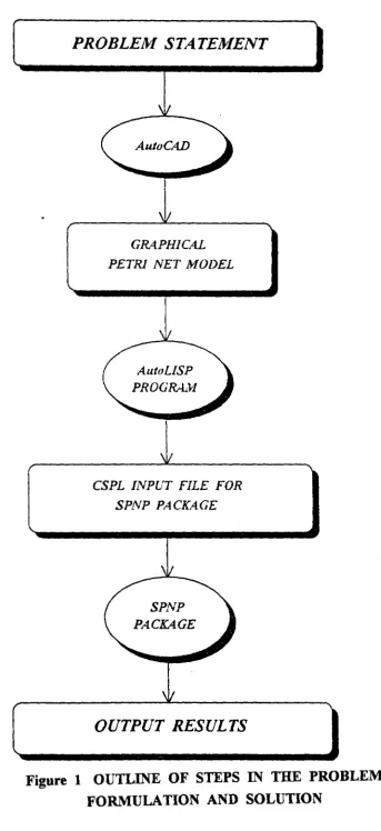
In this paper a manufacturing system using two processing machines and an assembly machine is modelled using Stochastic Petri nets. This stochastic Petri net is analyzed to obtain performance indices. The tool used is the Stochastic Petri Net Package ( SPNP ), developed at Duke University by Trivedi and coworkers, in which the stochastic Petri nets are described in the input language for SPNP called CSPL ( C-based SPN Language). A drawback with the SPNP package is that it does not have a graphical interface.

PROBLEM STATEJttJENT

Auto CAD

GRAPHICAL

PETRJ NET /ltf ODEL

CSPL INPUT FILE FOR SPNP PACKAGE

SPNP

OUTPUT RESULTS

2

STOCHASTIC AND GENERALISED STOCHASTIC

PETRI NETS

A Stochastic Petri net can be defined as a tuple;

SPN = { P, T, II(.), I(.), 0(.), H(.), W(.), Mo }, (1)

where PN = { P, T, II(.), 1(.), 0(.), H(.), Mo } is the Petri net underlying

the SPN defined above [ Ajmone et al. (1991) ]. The function W(.) defines the stochastic component of the SPN model, and it maps transitions into real positive numbers. For the transition ti E T, the function W(.), represented as wi is called the 'rate' of the transition ti. In the case where several transitions are simultaneously enabled, the transition that has the shortest delay time will fire first. An enabled transition ti will not fire when it becomes disabled because of the firing of other transitions, before its firing time di has passed. A set of enabled transitions is said to be conflicted at time 't, if for any pair of transitions

1i

1i

In order to cope with the state-space explosion problem, stochastic Petri nets have been extended to a class of generalized stochastic Petri nets ( GSPN ), [ Tadao Murata (1989)]. In a GSPN there are two types of transitions:

• Time delays associated with transitions are exponentially distributed random variables. These are called timed transitions, and are represented as bars,

( - - ) .

• Time delays associated with transitions are deterministically zero. These are called immediate transitions and are used to represent logical controls or activities whose delay times are negligible, compared with those associated with timed transitions. Immediate transitions are represented as boxes, ( I I ).

6 transition firings is called a loop ( of vanishing markings ). A loop is said to be absorbing, if no marking in it reaches a marking outside the loop, otherwise the loop is said to be transient. An absorbing loop is considered an error. The dynamic behaviour of the GSPN is equivalent to a continuous-time stochastic process. In a vanishing marking, the probability values associated with the enabled immediate transitions are used to probabilistically select the enabled immediate transitions to fire. The time spent in any vanishing marking is deterministically equal to zero. Reduction of the state-space can be achieved by discarding vanishing markings that correspond to some intermediate states in which the system spends zero or negligible amount of time.

The Stochastic Petri net model is analyzed by studying the structural properties of the underlying Petri net and by computing the steady state or transient probability distribution of the associated stochastic model. The SPN model can be translated into continuous-time Markov chains, [ see Ajmone et al. (1991) ]. There are a large number of techniques available to analyze this kind of stochastic model.

Due to the memoryless property of the exponential distribution of firing delays, the reachability graph of a bounded stochastic Petri net is isomorphic to a finite state Markov Chain. The Markov Chain of a SPN can be obtained from the reachability graph of the Petri net underlying the SPN. The Markov Chain state space is the reachability set R(M0 ), of the Petri net.

Suppose the delay di associated with transition ~ is represented by a non-negative continuous random variable X with the exponential distribution function :

Fx(x)

=

=

The average delay time is given by :

CIC> 0 0

d·

J [

1 - F (x) ] dx

0 X

- J

e-wix dx = 1 I W·

0 l (2)

Where wi is the firing rate of transition ti [ Tadao Murata (1989)]. The transition rate from state Mi to state Mj is given by :

( for transitions t_1, t_{2, .} . . . transforming Mi into Mj ). The square matrix Q

= [

I

I

For the reversible stochastic Petri net, i.e. Mo E R(Mi) for every Mi E R(M_{0 ),} it

is possible to compute the steady-state probability distribution TI, [see, Tadao Murata (1989) ] from the continuous-time Markov chain, by solving the linear system,

s

TIQ=O, "'"' _L..J 1t· = 1

I ' (3)

i =I

where xi is the probability of being in state Mi and II= ( x_1, x_2, . .. . x₈ ). From

the steady-state distribution

n,

1. The probability of a particular condition.

Let A be the subset of the reachability set R(M0 ), satisfying a particular

condition. Then the probability of satisfying the condition A is given by,

p {A}=

L

1t· _I

2. The expected value of the number of tokens in a place Pi·

(4)

Let B(i,n) be the subset of R(M0 ) for which the number of tokens in a

k-bounded place Pi is n. Then, the expected value of the number of tokens in place Pi is given by,

k

E (md -

L

8

3. The mean number of firings of a transition tj, in unit time.

Let Bj be the subset of R(M0 ) in which a transition tj is enabled. Thus, the mean

number of firings of transition tj in unit time is given by,

f. =

J (6)

3

APPLICATION OF GENERALIZED

STOCHASTIC PETRI NETS

Real-time control systems are, in general, highly concurrent by nature. Because of their conceptual complexity, the designer of such systems needs some help from specification through to implementation. Petri nets are among the most promising formal tools for managing concurrency. This approach needs a specification or modelling formalism in which the assertions expressing the properties under study can be mathematically proved. Thus it must be clear and unambiguous. The important features for a good specification formalism are, [ Silva (I 989) ] :

*

• Practical expressive power, allowing the model building by means of stepwise refinement and modular composition methodologies.

• Clear and explicit modelling of activities and events.

• Graphical representation, as a way to improve the necessary dialog between designers and users, and as a way to facilitate documentation tasks.

*

• The existence of a powerful analysis and verification theory to allow the formal verification of the specification. Properties can be of logical or qualitative nature such as dead-lock freeness, mutual exclusion, liveness, boundedness, reachability, fairness, etc., or performance indices or quantitative properties such as upper I lower bounds, average behaviour for throughputs, working ratios, queue lengths, etc ..

• The existence of computer packages to help the designer during the design, analysis and verification phases.

• Petri nets provides an easy-to-understand and ngorous semantic of true concurrency.

• There exists an extensive body of theory that allows formal validation of Petri net models, such as boundedness and liveness properties, mutual exclusion, synchronic distance, fairness, etc.

• The graphical representation of Petri net models make them a well suited support for the necessary dialog between users and designers.

• The independence of implementation techniques. There are a wide variety of applications from programmable logic controllers to ADA - based implementations.

There are several steps to be followed in the study of a system using the GSPN approach, [ Ajmone et al. (1991)].

• The model must be constructed using a structural technique, using either top-down or bottom-up approach, depending on the type of the system to be modelled.

• The constructed model must be validated using structural analysis methods, possibly proving some behavioural properties of the model.

• The performance indices required, must be defined, in terms of GSPN markings and the transition firings.

• The reachability set and the reachability graph are generated, in order to obtain the continuous-time Markov chain, associated with the GSPN model.

• The Markov chain is solved.

• The performance indices are computed from the Markov chain solution.

By using a Petri net based approach, formal specification and formal validation of the system under consideration can be easily achieved. If the model is a good abstraction of the system, the analyst can quickly c.arry out trade-off studies, answer "what if' questions, perform sensitivity analysis and design alternatives. As running of simulations can sometimes be very time consuming, it is useful for the system designers to use analytic models, instead of, or in addition to simulation models. Each kind of analytic model is well suited for some particular set of applications, but every model type also has its limitations.

Modelling tools for designing complex systems must be selected such that, qualitative and quantitative analysis can be achieved in an efficient manner. Markov chains and queuing network models have been used for the exact quantitative analysis. As

discussed above, Petri net models have been introduced for designing, validating and computing performance measures of complex systems. In these models, either stochastic or deterministic timing interpretation is added to the autonomous Petri net scheme, as well as a given decision policy for the resolution of conflicts. Petri nets provide synchronization capabilities that are not allowed with classical queuing networks.

Stochastic Petri net models are 'state-space' models, that is, the analysis requires the generation of a 'state-space', an enumeration of the possibilities of what can happen to the system, [ Sahner et al. (1991) ]. However, certain kinds of real-life system structures and dependencies violate the assumptions made by these models. State-space methods, such as those based on Markov and semi-Markov models, can capture system dependencies. They are very widely applicable, but a possible large size of state-space can be a problem during model generation and model analysis. Another important feature is that the possibility to set up multiple models for the same underlying system. This is a good validity check for both the construction and analysis of the models.

One decomposition approach is to decompose the system into subsystems and an SPN sub-model for each subsystem is developed. Then an overall model is composed from the constituent sub-models, talcing into account various interactions among subsystems. This approach consists of taking advantage of the natural decomposition by solving subsystems in isolation and exchanging solution components as and when required.

In model reduction, some of the places and I or transitions which will not have any effect on the numerical results, are removed from the net model. As an example, for the computation of the numerical results the GSPN is simplified by eliminating the immediate transitions. This results in a small reachability set and a small reachability graph, but it does not affect the size of the continuous time Markov chain ( CTMC) or the numerical results. In this approach the execution time and memory requirements savings are substantial.

The cost evaluation for the use of tools, there are two relevant aspects, [ Velilla et al. (1988) ]. The first aspect is the extra memory occupation, and the other is the time overhead in execution. Extra memory occupation is estimated based on the net structural parameters, such as the number of transitions ( m ), number of places ( n ), the amount of synchronization ( number of input places per transition f_{5 ),} the amount of parallelism ( number of output places per transition fp ), the amount of descendence ( number of output transitions per place fd ), and the amount of ascendance ( number of input transitions per place f_{8 )}. Of course, not all these

parameters are independent. In particular,

and

fp.

fa.

4

APPLICATION OF PETRI NETS TO

MANUFACTURING SYSTEMS

Design and Per/ ormance Analysis

The design of a manufacturing system requires extensive performance evaluation, to be able to decide among alternatives. Typical performance figures are throughputs ( product rates ), work in process and time span for each product, machine utilizations ( use ratios ), queue lengths or time distributions to access machines or transport subsystems, and so on. Alternatives to be considered at this level are : different layouts and transport systems, number of machines in a given work station, machines of different speeds and stores of different sizes, for example.

The introduction of stochastic or deterministic timing specification is essential if we want to use Petri net models for the performance evaluation of manufacturing systems. Since Petri nets are bipartite graphs, there can be two ways of introducing the concept of time in them, namely, associating a time interpretation with either places or transitions. Since transitions represent activities that change the state ( marking ) of the net, it seems natural to associate a duration with these activities ( transitions ). This allows the modeller to set up and solve a variety of model types, to compare results for different models of the same system, to see how altering system parameters affects measures of effectiveness of the system, and to experiment . with modelling techniques.

The instances of exceptional situations such as emergency stoppages due to

breakdowns, discarding of products, etc., can also be represented in the Petri net model for the manufacturing system. The occurrences of these exceptional situations can alter the net state and abort the tasks associated with transition firings. Constraints in a manufacturing system can define preferences relative to the time intervals surrounding the operations. Also some local constraints can define local preferences associated with the orders and resources involved in the conflict ( e.g. order priority, machine reliability, etc. ). They admit a certain amount of flexibility in interpretation. In practice some of these problems are considered prior to execution, in producing the production schedule, while others involve problems at a decision -making level (i.e. in which order should two waiting products be loaded onto a free machine ).

The integration of control functions of manufacturing systems require the identification of the following characteristics of such a system, [ Dewasurendra ,et al. ( 1991) ]

• Some common modelling environment for the different functions.

• Possibility to carry out substantial structural changes in a part of the system without affecting the whole system.

• Possibility of quick reaction to external events.

• Efficient communication among modules of the system.

• Ability to generate efficient action plans in the absence of well defined goals or

criteria.

• The ability to work with estimated parameters (temporal, for instance).

• The ability to test the action plans in simulation.

• The ability to revise action plans locally.

resulting in multiple production routes for products, large variation m production

batch sizes, tool capacity constraints, and the random failure of the resources. From

the point of view of the operations, a machine can perform an operation without

changing its current tool configuration or it can demand a set-up operation before

starting the given operation. The behaviour of all machines can be represented by

linear combinations of these two elementary behaviours. Thus the part of the Petri net

which corresponds to the Generic Machine will not change in its structure for different

manufacturing systems.

order arrives

order is waiting

processing starts

operator is idle waiting for work

order is being processed by the operator

processing is complete

using the machine

machine is idle, waiting for work

order is complete

order is delivered

Figure 2 PETRI NET MODEL OF A MANUFACTURING SYSTEM

Figure 2 represents a behavioural model of a manufacturing system which consists of

a Petri net. Its vision of the system state at any time is defined by the net marking. The

evaluation of the system state is achieved by firing transitions. The net's transitions are

defined with tasks to be done at the plant level. Firing a transition induces the

Reliability of Manufacturing Systems

Let us assume that the manufacturing system is able to detect a machine failure and reconfigure itself automatically. The system can still operate as long as 'enough' machines are available, which depends on the structural design of the system. The trade-offs involved in terms of system's reliability are as follows, [ Sahner et al.

(1991)] :

• The number of machinery needed to continue operations depends on the particular system design. System reliability is higher, if fewer machine items are required for the process. But the designing of a system requiring fewer number of machinery may increase the capital cost of machinery and design cost.

• Another arrangement may be to design a system with dedicated machines for some operations and some machines for multiple operations. This system could potentially have better performance than the first design, but it could be less reliable.

5

PROBLEM DESCRIPTION AND THE PETRI NET MODEL

In this paper a roller door manufacturing system is modelled using Petri nets. Figure 3

shows the layout diagram of the manufacturing facility. The system consists of two

loading bays, one for galvanised material and the other for coloured material, where

the raw materials are loaded onto the roll forming machines. Two roll forming

machines produce the 'curtains', one for a galvanised finish and the other for colours.

The galvanised roll former produces curtains in galvanised finish as and when orders

for galvanised doors are received. The colour roll former produces curtains in different colours depending on the number of orders for each colour. The colour roll former is

loaded with a certain colour when an economical quantity of orders ( the buffer size

for coloured door orders ) have been received for that colour. The economical

quantity for colour doors may be determined based on the following criteria:

• Minimize wastage of material due to change over of colour.

• The demand for different colours.

• Urgent orders for certain colours.

The processing time for roll forming of material for orders is not a constant. This is an important reason why Stochastic Petri nets may be used in the modelling. As the curtain is made by joining 950 mm wide panels, the processing time for an order varies

according to the door height and the door width.

There is a separate facility for the manufacture of drum assemblies for the doors. The

drum assemblies are basically the same for all types of doors. Again the processing

time varies according to the door measurements, as the number of springs varies.

Roll formed panels are seam-joined and assembled to the roller drum using the

assembly machine. This assembly time also varies according to the door size. The same

assembly machine is used for galvanised and colour doors. The assembled doors are sent to the dispatch bay for loading to the delivery trucks.

It is required to find out the optimum quantity of orders to be processed for one cycle of operation ( a normal working day ), and to determine the average queue lengths of

machines. This can be done in a manner as outlined in Section 2 and using in particular

equations (2) - (6). Also the buffer size for coloured door orders is to be determined.

In this analysis the following assumptions were made :

• Interarrival time for orders is considered to be zero, as all the orders to be

processed for a day are from the previous day.

• Processing times and repair or maintenance times are assumed to be exponentially

distributed.

• Movement of roll formed panels to the assembly machine is considered very small.

GALV.·

LOADING

GALV.

ROLL FORM.

ASSEMBLY

BUFFER

ASSEMBLY

MACHINE

COLOUR

ROLL FORM.

DISPATCH

Figure 3 LAYOUT DIAGRAM OF THE ROLLER DOOR

6

THE PETRI NET MODEL

The Petri net model for the 'Roller Door' manufacturing system described is shown in

Figure 4 and Figure 5. This Petri net is drawn using the AutoCAD design and drafting

package incorporating attribute blocks. Use of AutoCAD and AutoLISP to enhance

the modelling power of Petri nets is described in Appendix A.

The Detailed Petri Net Model

Tokens in the place p_order represent the receipt of orders for roller doors of all

types. The immediate transitions t_gal, t_gray, and t_brown, with the probability

values assigned to them are used to logically represent the distribution of orders for

galvanised finish, gray colour, and brown colour doors. Tokens in the places

p _gal_ buf, p _gr_ buf, and p _ br _buf represent the orders for different finishes in

respective buffers awaiting processing.

A token in each place p _ml _free and p _ m2 _free represent the idling state of the

galvanised roll former and of the roll former for coloured material respectively. Firing

of the immediate transition t_gal_ml_set represents the assigning of the galvanised

roll former to produce galvanised panels. It is assumed that this machine is always

loaded with galvanised material. A token in the place p_gal_in_ml represents the roll

forming of galvanised panels for an order. Firing of the timed transition t_gal_ml_rel

represents the end of processing, and the release of the roll former to the idling state.

Tokens in the place p_gal_wait_m3 represent the panels for galvanised finish orders

awaiting assembly. It is important here to note that the number of panels for an order

is usually between three to seven depending on the door height, and the length of a

panel for an order is the same, but may be different from order to order.

Firing of the immediate transition t_gr_m2_set ( t_br_m2_set ) represents the

assigning of the second roll former for gray ( brown ) coloured orders. Only one out of

these two transitions will fire when there are 'Y' tokens ( number of orders for each

colour ) in the places p _gr_ buf or p _ br _ buf. The quantity 'Y' ( the batch size or the

buffer size ) is to be determined for the optimal operation of the system. Firing of one

of these transitions will remove 'Y' tokens from the place p _gr_ buf ( p _ br _ buf) and

assigns 'Y' tokens to the place p_gr_in_m2 ( p_br_in_m2 ). This represents the roll

20 the input and output arcs of transition t_gr_m2_set ( t_br_m2_set) with a weight of magnitude 'Y'. Firing of the timed transition t_gr_end ( t_br_end) represents the end of processing of one order for gray colour. Roll formed panels go to the buffer represented by the place p_col_wait_m3 and await assembly. The number of tokens in this place represent the number of coloured orders awaiting assembly.

Also the firing of the timed transition t_gr_end ( t_br_end ) places a token in the place p_gr_end ( p_br_end ). When 'Y' tokens are collected in the place p_gr_end ( p_br_end ) the immediate transition t_gr_m2_rel ( t_br_m2_rel ) is enabled and can fire, indicating the release of the roll former for coloured panels to the idling state, after processing 'Y' gray ( brown ) orders. The processing of a batch of 'Y' orders is represented by assigning the input arc to the immediate transition t _gr_ m2 _rel ( t _ br _ m2 _rel ) with a weight of magnitude 'Y'.

Now the firing of the immediate transition t_gal_m3 ( t_col_m3 ) assigns the assembly machine for the assembly of galvanised ( coloured ) panels to produce galvanised ( coloured ) finish doors. A token in the place p _gal_ in_ m3 ( p_col_in_m3) represents the assembly process of galvanised (coloured) panels for an order. The firing of the timed transition t_gal_m3_rel ( t_col_m3_rel) represents the completion of the assembly process of a galvanised ( coloured ) finish door, and the release of the assembly machine to the idling state.

p_order

--Lgroy Lbrown

p_gr_buf p_br_buf

p_m1_free p_m2._free

y _y

Lgr_m2._set Lbr_m2._set

y

y

p_gaLin__m 1 p_gr_in__m2

LgaLm1_rel

p_gaLwoiLm3 p_olLwoiLm3

LgoLm3 Lo1Lm3

p_goLin__m3 p_a1Un__m3

LgaLm3_rel Lo1Lm3_rel

p_producLreody

Lexit

22

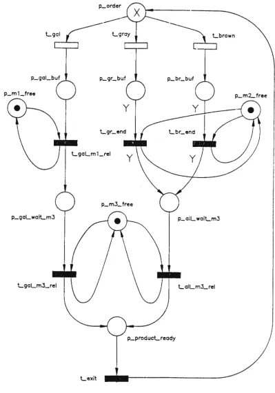
The Modified Petri Net Model

The Petri net model described in Figure 4 gives a very good graphical representation

of the system being modelled. The model consists of places, immediate transitions, timed transitions, input arcs and output arcs. The immediate transitions were used as

logical controls and to represent activities which consume negligible amount of time.

As the number of nodes ( places and transitions ) in a Petri net increases, the time

taken to analyze the net also increases, due to the state space explosion. The analysis

time can be reduced significantly by reducing the number of nodes in the net model.

This can be achieved by deleting some of the immediate transitions and places which are used only for logical control of the net, but do not have any effect on the

analytical results.

In the previous net model, the immediate transitions t_gal, t_gray, and t_brown

cannot be removed from the net model as they represent the probabilistic distribution of orders for different finishes of doors.

The removal of the transition t_gal_ml_set and the place p_gal_in_ml will not have

any effect on the analysis. This part of the net has to be rearranged as shown in Figure

5. The removal of the immediate transitions t_gr _ m2 _set and t_ br _ m2 _set together with places p_gr_in_m2 and p_br_in_m2 however, has to be done carefully as a batch of orders ( 'Y' ) is involved here. This is achieved by multiplying the time delays

associated with the timed transitions t_gr_end and t_br_end by the batch size ( 'Y' ) and assigning the input and output arcs of these transitions a weight equal to the batch size ( 'Y' ). Also by introducing input and output arcs (with weights of magnitude

one) between t_gr_end ( t_br_end) and p_m2_free, the assignment and the release of the roll former for coloured panels can be represented. The timed transition

t_gr_end ( t_br_end) in the modified net will be enabled when there are 'Y' tokens in

the place p_gr_buf ( p_br_buf ). Now the firing of the timed transition t_gr_end ( t_br_end) ends the processing of 'Y' gray (brown) coloured orders, depositing 'Y'

tokens in the place p_col_wait_m3, and releases the roll former to the idling state.

The tokens in the place p_gal_wait_m3 ( p_col_wait_m3) represent the galvanised (coloured) orders awaiting assembly. The firing of the timed transition t_gal_m3_rel

( t_col_m3_rel ) represents the end of assembly of a galvanised finish ( coloured )

The number of tokens in the place p _product_ ready represent the completed doors

of all types, awaiting delivery. The firing of the timed transition t_ exit represents the

end of loading of a door. This transition is connected to the place p _order by the

output arc for the steady state operation.

p_order

Lgol

p_gol_buf p_gr_buf p_br_buf

p_m1_free _{p_m.2_free}

y

Lgr_end Lbr_end

LgoLm1_rel

_y

y

p_mJ_free

p_gaLwait_mJ _{p_alLwoiLmJ}

LgcLmJ_rel _{LolLmJ_rel}

p_producLrecdy

Lexit

7

ANALYSIS AND RESULTS

In order to reduce the complexity of the analysis, the GSPN model was structurally

reduced before approaching the solution phase. In the reduction process most of the

immediate transitions were eliminated as described in Section 6. The advantages

obtained with the reduction are that by reducing the vanishing markings the complexity

is reduced in the solution of the continuous-time Markov chain underlying the GSPN.

In order to numerically solve, with acceptable time and space complexity, the

Markovian model derived from a GSPN description is in the restriction to exponential

distributions and finite buffer ( queue ) sizes, and in the model dimensions. For this

reason, only exponential distributions were considered in the model for the different

processing times. Also the maximum number of orders ( tokens ) were limited to a

smaller number. The analysis process was repeated using different number of tokens in

the order buffer, starting from 6 and increasing in steps of 2 to a maximum of 20. By

plotting the results into line graphs, it was possible to study the behaviour of the

system.

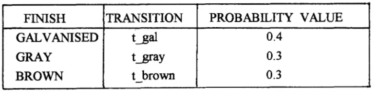
The sales data for the past six months were analysed to determine the distribution of

different finishes for doors being manufactured. This distribution is represented by

assigning probability values to the following transitions.

FINISH TRANSITION PROBABILITY VALUE

GALVANISED t_gal 0.4

GRAY t_gray 0.3

BROWN t brown 0.3

Table 1 TRANSITION PROBABILITIES

The mean processing times were obtained by averaging the processing times for the

past six months. The reciprocal of these values ( see equation (2) ) give the rate values

needed for the GSPN. Table 2 gives the mean processing times and the processing

25

PROCESS TRANSITION :MEAN TI:ME RATE VALUE

(min.) ( sec.-1)

GAL. ROLL FORMING t_gal_ml_rel 15.0 1. llE-3

GRAY ROLL FORMING t_gr_end I 20.0 8.33£-4

BROWN ROLL FORMING t br end _{- -} 20.0 8.33£-4

GAL. PANEL ASSEJ\IBL Y t _gal_ rn3 _rel 10.0 1.67£-3

COL. PANEL ASSEMBLY t all m3 rel 15.0 1. llE-3

- -

-LOADING (DISPATCH ) t exit 5.0 3.33£-3

Table 2 MEAN PROCESSING TIMES AND RATES

In the SPNP input file ( CSPL ) the predefined function pr_ expected is used to

output the information about the places and transitions which represent manufacturing

functions to be studied.

For example, to detennine the average queue length for the assembly machine for

coloured doors, the following functions were used (equation (5) ):

reward_type qlenallmJ() { return(mark("p_all_wait_mJ"));}

pr_expected("Ave. Q. Len. of Colours Awaiting Assembly", qlenallm3);

To determine the average utilization of the assembly machine by the coloured panels:

reward_type utilm3all() { retum(enabled("t_all_m3_rel"));}

pr_expected("Utilization of Assembly Machine for Colours", utilm3all);

To determine the average throughput of coloured doors (equation (6) ):

reward_type tputallO { return(rate("t_all_m3_rel"));}

pr_expected("Average Throughput of Coloured Doors", tputall);

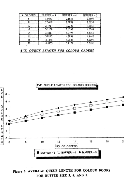
The results obtained are shown in Figures 6 to 11 and the curves plotted using these values versus the number of tokens ( number of orders for doors ) in the order

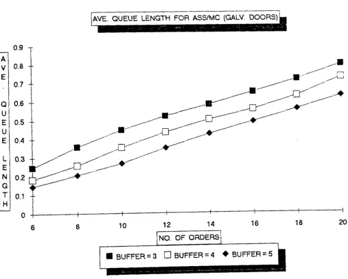
buffer. Figures 6 and 7 show the average queue length for processing color doors and

average queue length for assembly machine ( for galvanised doors ), respectively for

26

and average utilization of assembly machine by coloured doors, respectively for buffer

size 3, 4 and 5. Figures 10 and 11 show the average throughput of galvanised doors

and average throughput of coloured doors, respectively for buff er size 3, 4 and

5. The average queue length is given as the average number of doors ( tokens )

waiting at a particular station. The average throughput is given as the average number of doors ( tokens ) per second.

The impact of the buffer size on the results is smaller as the number of orders

increases. This is because the system tends to get saturated as the number of orders increases. In this situation the buffer size can be determined considering the other

factors such as priority orders. Another important fact to be observed here is that the

optimal capacity of this manufacturing system is around 20 orders for a cycle of

operation. Any increase in the number of orders beyond 20 will not have any

A

v

E

5

E 1 N

1;10

l!iJ

#ORDERS BUFFER=3 BUFFER= 4 BUFFER=5 6 1.9643 2.1856 2.3897

8 2.3648 2.7881 3.0135

10 2.7517 3.2222 3.6157

12 3.1109 3.6292 4.0744 14 3.4411 4.0195 4.4955

16 3.8192 4.3831 4.8442

18 _' 4.1845 4.7536 5.2091 20 4.4873 5.1178 5.5691

.

AVE. OUEUE LENGTH FOR COLOUR ORDERS

!AVE. QUEUE LENGTH FOR COLOUR ORDERS'

8 10 12 14 16 18

NO. OF ORDERS

• BUFFER= 3

0

+

Figure 6 AVERAGE QUEUE LENGTH FOR COLOUR DOORS FOR BUFFER SIZE 3, 4, AND 5

I 0.9 A

v

E

0.7

Q 0.6

ul

E 0.5

u

E 0.4

6

28

#ORDERS BUFFER 3 BUFFER 4 BUFFER 5

6 0.2455 0.1832 0.1461

8 0.3576 0.2581 0.2064

10 0.4491 0.3541 0.2682

12 0.5242 0.4357 0.3521

14 0.5849 0.5037 0.4263

16 0.6512 0.5601 0.4926

18 0.7216 0.6319 0.5603

20 0.8019 0.7313 0.6329

AVE. QUEUE LENG11l FOR ASS/J-IC (GAL

1'

:

AVE. QUEUE LENGTH FOR ASS/MC (GALV. DOORS)

8 10 12 14 16 18

I I

NO. OF ORDERS\

• BUFFER::: 3

0

+

Figure 7 AVERAGE QUEUE LENGTH FOR ASSEMBLY MACHINE

( GALV. DOORS ) FOR BUFFER SIZE 3, 4, AND 5

A

v

u

T

I

L

I

z

T

I 0 N

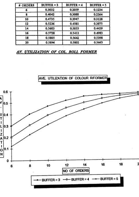
#ORDERS BUFFER-3 BUFFER=4 BUFFER=5

6 0.3032 0.2059 0.1234

8 0.4042 0.3088 0.2264

10 0.4735 0.3947 0.3128

12 0.5236 0.4581 0.3815

14 0.5603 0.5053 0.4459

16 0.5728 0.5412 0.49&3

18 0.5805 0.5642 0.5398

20 0.5896 0.5802 0.5663

AV. UTJUZATION OF COL ROLL FORMER

!AVE. UTILIZATION OF COLOUR RIFORMER'

0.6

0.5

0.4

0.3

0.2

0.1

0

6

1

0.9

u

I 0.7

AL 0.6

v'

A · T 0.4

I

0 0.3

N 0.2

0.1

30

#ORDERS BUFFER=3 BUFFER=4 BUFFER-S

6 0.4551 0.3198 0.2084

8 0.6066 0.4634 03518

10 0.7107 0.5925 0.4695

12 0.7858 0.6876 0.5816

14 0.8411 0.7584 0.6694

16 0.8702 0.8123 0.7483

18 0.8913 0.8548 0.8062

20 0.9034 0.8861 0.8576

AV. UTIUZATION OF ASS/MC BY COL DOORS

!Av. UTILIZATION oF ASS/Mc ev coLouR

oooRS

I

0

' 6 8 10 12 14 16 18

!No OF ORDERS!

Figure 9 AVERAGE UTILIZATION OF ASSEMBLY MACHINE BY COLOURED DOORS, FOR BUFFER SIZE 3, 4, AND 5

# ORDERS BUFFER=3 BUFFER.=4 BUFFER.=5

6 0.00029 0.000219 0.000129

8 0.00043 0.000341 0.000249

10 0.00055 0.000441 0.000357

12 0.00062 0.000509 0.000431

14 0.00065 0.000561 0.000495

16 0.00067 0.000601 0.000542

18 0.00068 0.000638 0.000598

20 0.00069 0.000665 0.000634

AV. THROUGHPUT OF GAL DOORS

0.0007

A

v

E'

. 0.0005

T H R 0

u

G

H

p

u

T

0.0004

0.0003

0.0002

0.0001

0

6 8 10 12 14 16 18 20

'NO OF ORDERS!

Figure 10 AVERAGE THROUGHPUT OF GALVANISED DOORS

0.001

A 0.0009

v

E 0.0008

. 0.0007

T 0.0006

H

R 0.0005 0

u

H 0.0003

p 0.0002

u

T 0.0001

32

# ORDERS BUFFER=3 BUFFER=4 BUFFER=S

6 0.0005 0.000355 0.000231

8 0.00067 0.000511 0.000391

10 0.00079 0.000661 0.000521

12 0.00087 0.000763 0.000646

14 0.00093 0.000842 0.000743

16 0.00095 0.000902 0.000833

18 0.00096 0.000913 0.000874

20 0.00097 0.000924 0.000902

AV. THROUGHPUT OF COLOUR DOORS

jAv.

0 + - - - 1 - - - - + - - - + - - - - + - - - + - - - 1 r - - - t

6 8 10 12 14 16 18

jNO OF ORDERS!

_ _ B_U_F_F_E_R_=_S...,

Figure 11 AVERAGE THROUGHPUT OF COLOURED DOORS FOR BUFFER SIZES 3, 4, AND 5

33

8

CONCLUSIONS

In this paper a summary of the structural and temporal definitions that lead to the

Generalised Stochastic Petri Net approach for the modelling of manufacturing systems

has been presented. Also the problem of computing the steady-state performance

measures of some classes of manufacturing systems modelled with Generalised

Stochastic Petri Nets has been addressed. As an example, a roller door manufacturing

system was modelled and its performance measures such as the queue length,

throughput and utilisation values were computed for different set-ups of the system. It

has been shown how the use of Petri nets and Petri net Tools can help the examination

of different aspects of a manufacturing system design and performance analysis.

It has been shown in the literature that GSPN permit a modular approach to the model

development process, using either a top-down or a bottom-up approach [ Hatono et

al. (1989) ], in which the specification of the model components can be represented in greater detail. Also the modular approach helps in tackling the high memory

requirement and long CPU times needed for the analysis of very large systems. Use of

a coloured Petri net tool would make the net much simpler by reducing the number of

places and transitions.

For the generation of the Petri net model and the input file for the SPNP package,

AutoCAD Release 9 and AutoLISP Release 9 were used. Now AutoCAD and

REFERENCES

Ajmone M., G. Balbo, G. Chiola, G. Conte, S. Donatelli and G. Franceschinis (1991), An Introduction to Generalized Stochastic Petri Nets. Microelectronics and Reliability, Vol. 31, No. 4, pp 699-725, 1991.

AutoCAD Release 9 ( 1987), Reference Manual, AUTODESK, INC.

AutoLISP Release 9 (1987), Programmer's Reference, AUTODESK, INC.

Ciardo Gianfranco and Jogesh K. Muppala (1992), Reference manual for the SPNP Package, Version 3. 1. Dept of Electrical Engineering, Duke University, Durham, NC (USA).

Dewasurendra Devapriya, Descotes-Genon Bernard and Ladet Pierre ( 1991 ), A Petri Net Based Blackboard Type Architecture for FMS, Laboratoire d'Automatique de Grenoble, Martin d'Heres (France).

Hatono Itsuo, Norihiro Katoh, Keiichi Yamagata and Hiroyuki Tamura (1989), Modelling of FMS under Uncertainty Using Stochastic Petri Nets. Proceedings of the 3rd International Workshop of Petri Nets and Performance Models, Kyoto

(Japan), December 1989, pp 122-129.

Murata Tadao (1989), Petri Nets: Properties, Analysis and Applications. Proceedings of the IEEE, Vol. 77, No. 4, pp. 541-580.

Sahner Robin A and Kishor S. Trivedi (1991), A Toolchest for Stochastic Models.

Duke University, Durham (USA).

Silva Manuel and Robert Valette (1990), Petri Nets and Flexible Manufacturing.

Research Report, GISI-RR-90-3, Departamento de lngenieria Electrica e

Informatica, Universidad de Zaragoza, Spain.

35

APPENDIX A

GRAPHICAL INTERFACE

The popular PC based design and drafting software package, AutoCAD is used to enhance the modelling power, by graphically generating the Petri net model. AutoLlSP, which is an extension to AutoCAD is used to read the Petri net model from the graphic screen of AutoCAD and automatic generation of the source code for the SPNP package input file. Refer to Figure I for an overview of the problem solution plan.

AutoCAD Drawing

To draw the Petri net on the graphic screen, the AutoCAD entities called attribute blocks are used [ AutoCAD Release 9 (1987), Reference Manual]. An attribute is a drawing entity designed to hold textual data and to link that data to graphic objects ( blocks ) within the drawing database. Each time an attribute block is inserted into a drawing, the user will be prompted by the attribute to add textual information to that block. The textual information can be the name of the place, or the transition, number of tokens for a place, or the firing rate of a transition. This information will remain with that block forever. Later on, the data contained in these attribute blocks can be extracted and the information used to keep track of the objects in the drawing.

In this paper, attribute blocks are used to represent the "building blocks" of Petri nets, such as place, immediate transition, timed transition, input arc, output arc, and inhibitor arc. Following is an example of an attribute block used to represent a 'place'.

Block name

Usage

Attribute tag

prompt

Attribute tag

prompt

default value

PLACE

place

PNAME

(visible)

Place name

TOKEN

(visible)

No. of tokens

AutoLISP Program

AutoLISP is a subset of common LISP with many additional built-in graphics handling functions. AutoLISP is the programming language within AutoCAD that allows the writing of programs that will manage and manipulate the graphic and non-graphic data. [ AutoLISP Release 9 (1987), Programmer's Reference] AutoLISP lets users and AutoCAD developers write macro programs and functions in a powerful high-level language that is well suited to graphics applications.

A drawing database is structured exactly the same way as any other database. Its purpose is to describe a drawing in a non-graphic way. A drawing database file consists of records of alphanumeric descriptions of drawing primitives ( AutoCAD

drawing entities ). Here an AutoLISP program is used to extract and use data from

AutoCAD drawings of Petri nets. These data are the attribute blocks used to construct the Petri nets.

An association list is a list, structured so that it can be accessed by the "assoc"

function. The following AutoLISP program "entlst", will list all the entity association lists in a drawing :

( defun entlst

O

)

( setq e ( entnext ))

(while e

( print ( entget e ))

( terpri)

( setq e ( entnext e ))

)

; sets e to the first entity name ; loop as long as there are entities

; print the entity list

; new line

; set e to next entity

The AutoLISP program, entlst, is a basic loop structure that will look at every item in the drawing database. By inserting certain control statements in the middle of this loop structure, it is possible to cause the program to look only for drawing entities that meet certain criteria.

( setq enttyp ( cdr (assoc 0 ( entget e ))))

From the AutoCAD drawing of the Petri net consisting of attribute blocks, the

association lists are extracted using a program similar to "entlst". Only the necessary

information required for the SPNP input file is extracted from the association list,

38

APPENDIX B

STOCHASTIC PETRI NET PACKAGE

The Stochastic Petri Net Package ( SPNP) is a versatile modelling tool for solution of

stochastic Petri net ( SPN ) models. The stochastic Petri net models are described

[ Ciardo et al. (1992)] in the input language for SPNP called C-based SPN Language

( CSPL ). The CSPL is an extension of the C programming language, with some

additional constructs. The SPN models specified to SPNP are 'SPN Reward Models'

or stochastic reward nets ( SRN ), which are based on the 'Markov Reward Models'

paradigm. This provides a powerful modelling environment for dependability analysis,

performance analysis and performability modelling. The package allows the solution of

the SRN to obtain either steady-state metrics or transient metrics.

In addition to standard features available to describe the mechanisms of Petri net

models, this package has a few special features. Some of the special features are :

• The marking dependent enabling .function associated with a transition. The value

of this function is evaluated by the expression containing the marking(s) of one or

more places. If this function evaluates to 1, in a marking, then the transition ts

enabled, if the value is 0, then the transition is disabled.

• The marking dependent arc multiplicity. Arcs can have multiplicity which is not constant, but rather it is a function of the marking. This feature may help to ~educe

the size of the reachability graph, and it ·may allow compact models.

The SRN to be studied is described in a CSPL file, which is a C file specifying the

structure of the SRN and the desired outputs, by means of predefined functions, for

example, pr_std_average(); outputs, for each place, the probability that it is not

empty and its average number of tokens; for each timed transition, the probability that

it is enabled and its average throughput. The average throughput E[Ta] for transition

a is defined as ( equation ( 6) ) :

E[ Ta

l -

L

w

'

iER(a)

where R(a) is the subset of reachable markings that enable transition a, xi is the