Electronic Thesis and Dissertation Repository
4-7-2017 12:00 AM
Visual Transfer Learning in the Absence of the Source Data
Visual Transfer Learning in the Absence of the Source Data
Shuang Ao
The University of Western Ontario
Supervisor Charles X. Ling
The University of Western Ontario Graduate Program in Computer Science
A thesis submitted in partial fulfillment of the requirements for the degree in Doctor of Philosophy
© Shuang Ao 2017
Follow this and additional works at: https://ir.lib.uwo.ca/etd
Part of the Artificial Intelligence and Robotics Commons
Recommended Citation Recommended Citation
Ao, Shuang, "Visual Transfer Learning in the Absence of the Source Data" (2017). Electronic Thesis and Dissertation Repository. 4463.
https://ir.lib.uwo.ca/etd/4463
This Dissertation/Thesis is brought to you for free and open access by Scholarship@Western. It has been accepted for inclusion in Electronic Thesis and Dissertation Repository by an authorized administrator of
Image recognition has become one of the most popular topics in machine learning. With the development of Deep Convolutional Neural Networks (CNN) and the help of the large scale labeled image database such as ImageNet, modern image recognition models can achieve competitive performance compared to human annotation in some general image recognition tasks. Many IT companies have adopted it to improve their visual related tasks. However, training these large scale deep neural networks requires thousands or even millions of labeled images, which is an obstacle when applying it to a specific visual task with limited training data. Visual transfer learning is proposed to solve this problem. Visual transfer learning aims at transferring the knowledge from a source visual task to a target visual task. Typically, the target task is related to the source task, and the training data in the target task is relatively small. In visual transfer learning, the majority of existing methods assume that the source data is freely available and use the source data to measure the discrepancy between the source and target task to help the transfer process. However, in many real applications, source data are often a subject of legal, technical and contractual constraints between data owners and data customers. Beyond privacy and disclosure obligations, customers are often reluctant to share their data. When operating customer care, collected data may include information on recent technical problems which is a highly sensitive topic that companies are not willing to share. This scenario is often called Hypothesis Transfer Learning (HTL) where the source data
is absent. Therefore, these previous methods cannot be applied to many real visual transfer learning problems.
In this thesis, we investigate the visual transfer learning problem under HTL setting. Instead of using the source data to measure the discrepancy, we use the source model as the proxy to transfer the knowledge from the source task to the target task. Compared to the source data, the well-trained source model is usually freely accessible in many tasks and contains equivalent source knowledge as well. Specifically, in this thesis, we investigate the visual transfer learning in two scenarios: domain adaptation and learning new categories. In contrast to the previous methods in HTL, our methods can both leverage knowledge from more types of source models and achieve better transfer performance.
In chapter 3, we investigate the visual domain adaptation problem under the setting of Hypothesis Transfer Learning. We propose Effective Multiclass Transfer Learning (EMTLe)
that can effectively transfer the knowledge when the size of the target set is small. Specifically, EMTLe can effectively transfer the knowledge using the outputs of the source models as the auxiliary bias to adjust the prediction in the target task. Experiment results show that EMTLe can outperform other baselines under the setting of HTL.
Adaptation (GDSDA). Specifically, we show that GDSDA can effectively transfer the
knowl-edge using the unlabeled data. We also demonstrate that the imitation parameter, the hyper-parameter in GDSDA that balances the knowledge from source and target task, is important to the transfer performance. Then we propose GDSDA-SVM which uses SVMs as the base classifier in GDSDA. We show that GDSDA-SVM can determine the imitation parameter in GDSDA autonomously. Compared to previous methods, whose imitation parameter can only be determined by either brute force search or background knowledge, GDSDA-SVM is more effective in real applications.
In chapter 5, we investigate the problem of fine-tuning the deep CNN to learn new food categories using the large ImageNet database as our source. Without accessing to the source data, i.e. the ImageNet dataset, we show that by fine-tuning the parameters of the source model with our target food dataset, we can achieve better performance compared to those previous methods.
To conclude, the main contribution of is that we investigate the visual transfer learning problem under the HTL setting. We propose several methods to transfer the knowledge from the source task in supervised and semi-supervised learning scenarios. Extensive experiments results show that without accessing to any source data, our methods can outperform previous work.
Keywords: Visual Transfer Learning, Hypothesis Transfer Learning, Supervised Learning,
Semi-supervised Learning
Firstly, I would like to thank my advisor Prof Charles X. Ling for his patience and insightful guidance. He was always eager to discuss new ideas at any time help me understand the research and inspired me to thinking critically for the topic I was working on.
Thanks are also given to my colleagues: Yan Luo, Xiao Li, Bin Gu, Chang Liu, Robin Liu and Jun Wang for their collaboration and valuable discussions. Many thanks to Xiang Li. We worked together with many ideas and he is very helpful in many details of the papers we published together.
The Last gratitude is given to my families: my parents Dingan Ao and Liwen Yang, and my wife Jinglang Hu. Without their encouragements and supports, I am not able to pursuing my PhD degree in Western and finish this dissertation.
My research is supported by NSERC Grants and scholarship from the Universitys the School of Graduate Studies. This thesis would not have been possible without the generous resources provided by the Department of Computer Science.
Acknowlegements i
Abstract ii
List of Figures viii
List of Tables xi
1 Introduction 1
1.1 Overview for Image Recognition . . . 2
1.1.1 Preprocess. . . 2
1.1.2 Feature Extraction . . . 3
1.1.2.1 Hand Engineered Feature . . . 3
1.1.2.2 Representation Learning . . . 4
1.1.3 Classification . . . 6
1.2 Approaches in Visual Transfer Learning and the Limitations . . . 7
1.2.1 Intuition for Visual Transfer Learning . . . 7
1.2.2 Approaches for Visual Transfer Learning . . . 8
1.2.3 Limitation of Previous Methods . . . 9
1.3 Main Contribution . . . 10
1.3.1 Challenges . . . 10
1.3.2 Two Transfer Learning Scenarios . . . 11
1.3.3 Proposed Methods . . . 12
1.4 Summary . . . 12
2 Related Work 13 2.1 Classifiers for Image Recognition . . . 13
2.1.1 Binary Classification and Multi-class Classification . . . 13
2.1.2 Softmax Classifier . . . 14
2.1.3.3 Kernel SVM . . . 18
2.1.4 Convolutional Neural Networks . . . 20
2.1.4.1 Early Work with Convolutional Neural Networks . . . 20
2.1.4.2 Recent Achievements with Convolutional Neural Networks . 21 2.2 An Overview of Visual Transfer Learning . . . 22
2.2.1 Types of Transfer Learning from the Situations of Tasks . . . 23
2.2.2 Types of Transfer Learning from the Aspect of Source Knowledge . . . 24
2.2.3 Special Issues in Avoiding Negative Transfer . . . 26
2.3 Related Work in Hypothesis Transfer Learning . . . 28
2.3.1 Fine-tuning the Deep Net . . . 29
2.3.2 Hypothesis Transfer Learning with SVMs . . . 29
2.3.2.1 LS-SVM Classifier . . . 31
2.3.2.2 ASVM & PMT-SVM. . . 31
2.3.2.3 MULTIpLE . . . 34
2.3.3 Distillation for Knowledge Transfer . . . 34
2.4 Summary . . . 36
3 Effective Multiclass Transfer For Hypothesis Transfer Learning 37 3.1 Introduction . . . 37
3.2 Using the Source Knowledge as the Auxiliary Bias . . . 38
3.3 Bi-level Optimization for Transfer Parameter Estimation . . . 40
3.3.1 Low-level optimization problem . . . 41
3.3.2 High-level optimization problem . . . 42
3.4 Experiments . . . 43
3.4.1 Dataset & Baseline methods . . . 43
3.4.2 Transfer from Single Source Domain. . . 44
3.4.3 Transfer from Multiple Source Domains . . . 45
3.5 Summary . . . 46
4 Fast Generalized Distillation for Semi-supervised Domain Adaptation 50 4.1 Introduction . . . 50
4.2 Previous Work . . . 51
4.3 Generalized Distillation for Semi-supervised Domain Adaptation . . . 52
4.4 GDSDA-SVM . . . 57
4.4.1 Distillation with Multiple Sources . . . 57
4.4.2 Cross-entropy Loss for Imitation Parameter Estimation . . . 58
4.5 Experiments . . . 59
4.5.1 Single Source for Office datasets . . . 60
4.5.2 Multi-Source for Office datasets . . . 61
4.6 Summary . . . 62
5 Learning Food Recognition Model with Deep Representation 64 5.1 Introduction . . . 64
5.2 Tuning the Deep CNNs . . . 64
5.3 Layers in Deep CNN . . . 66
5.3.1 Convolutional Layer . . . 66
5.3.2 Pooling Layer . . . 66
5.3.3 Fully Connected Layer . . . 67
5.3.3.1 Rectified Linear Units (ReLUs) for Activation . . . 68
5.3.3.2 DropOut . . . 68
5.4 Experiment Settings . . . 69
5.4.1 Models . . . 69
5.4.2 Food Datasets . . . 70
5.4.3 Data Augmentation . . . 71
5.5 Discussion . . . 73
5.5.1 Pre-training and Fine-tuning . . . 75
5.5.2 Learning across the datasets . . . 77
5.6 Summary . . . 80
6 Conclusion 81 Bibliography 83 A Proofs of Theorems 94 A.1 Closed-form Leave-out Error for LS-SVM . . . 94
A.2 Converage of EMTLe . . . 95
B Configuration of GoogLeNet 98
1.1 Major procedure for image recognition. . . 3
1.2 Feature extraction using SIFT. . . 4
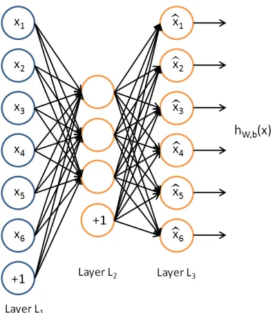
1.3 General Scheme of Auto Encoders. L1 is the input layer, possibly raw-pixel intensities. L2 is the compressed learned latent representation and L3 is the reconstruction of the given L1 layer from L2 layer. AutoEncoders tries to min-imize the difference between L1 and L3 layers with some sparsity constraint.. . 5
1.4 The architecture of ALEXNET (adopted from [58]). . . 6
1.5 An intuitive description for human to learn new concept: an okapi can be roughly described as the combination of a body of a horse, legs of the zebra and a head of giraffe. . . 7
1.6 Feature transformation. Transform the data in different domains into a aug-mented feature space. . . 9
1.7 Difference between two transfer learning scenarios . . . 11
2.1 One-vs-Rest strategy for multi-class scenario. A three classes problem can be decomposed into 3 binary classification sub-problems.. . . 14
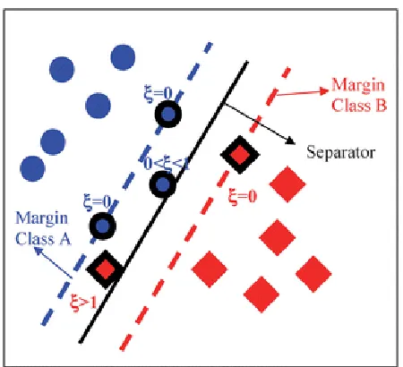
2.2 Support Vector Machine. . . 17
2.3 Slack variables for soft-margin SVM . . . 18
2.4 The hyperplane of SVM with RBF kernel for non-linear separable data. . . 19
2.5 Apart from the standard machine learning, transfer learning can leverage the information from an additional source: knoweldge from one or more related tasks.. . . 23
2.6 Two steps for parameter transfer learning. In the first step multi-source and single source combination are usually used to generate the regularization term. The hyperplane for the transfer model can be obtained by either minimizing training error or cross-validation error on the target training data. . . 25
2.7 Positive transfer VS Negative transfer. . . 27
2.8 Hierarchical Features of Deep Convolutional Neural Networks for face recog-nition. . . 30
i
model andβin is the hyperparameter (need to be estimated) to weigh the
aug-mented feature.φn(x) is augmented feature for then-th binary model.. . . 38
3.2 Demonstration of using the source class probability as the auxiliary bias to adjust the output of the target model. The source task is to distinguish the 4 pop cans while the target one is to distinguish the 4 pop bottles . . . 39
3.3 Bi-level Optimization problem for EMTLe. . . 41
3.4 Recognition accuracy for HTL domain adaptation from a single source (Part1). 5 different sizes of target training sets are used in each group of experiments. A, D, W and C denote the 4 subsets in Table 3.1 respectively. . . 47
3.5 Recognition accuracy for HTL domain adaptation from a single source (Part2). 5 different sizes of target training sets are used in each group of experiments. A, D, W and C denote the 4 subsets in Table 3.1 respectively. . . 48
3.6 Recognition Accuracy for Multi-Model & Multi-Source experiment on two tar-get datasets. . . 49
4.1 Illustration of Generalized Distillation training process. . . 52
4.2 Illustration of GDSDA training process and our “fake label” strategy. . . 53
4.3 An example of using GDSDA to generate distilled labels for the target data. . . 55
4.4 D+W→A, Multi-source results comparison. . . 61
4.5 Experiment results on DSLR→Amazon and Webcam→Amazon when there are
just one labeled examples per class. The X-axis denotes the imitation parameter of the hard label (i.e. λ1 in Fig 4.2) and the corresponding imitation parameter
of the soft label is set to 1−λ1. . . 63
5.1 Demonstration of Fine-tuning from ImageNet 1000 classes to Food-101 datasets. 65
5.2 Convolution operation with 3×3 kernel, stride 1 and padding 1.⊗denotes the
convolutional operator. . . 67
5.3 2×2 pooling layer with stride 2 and padding 0. . . 68
5.4 Dropout Layers. Adopted from Standford CS231n Convolutional Neural Net-works for Visual Recognition . . . 69
5.5 Inception Module. n×nstands for sizenreceptive field,n×n reducestands for
the 1×1 convolutional layer before then×nconvolution layer and pool pro j
is another 1×1 convolutional layer after the MAX pooling layer. The output
5.8 Visualization of some feature maps of different GoogLeNet models in different layers for the same input image. 64 feature maps of each layer are shown. Conv1 is the first convolutional layer and Inception 5b is the last convolutional layer. . . 76
2.1 Categories of our learning scenarios . . . 23
2.2 Relationship between traditional machine learning and different transfer learn-ing settlearn-ings . . . 23
2.3 Various settings of transfer learning. . . 24
3.1 Statistics of the datasets and subsets . . . 44
3.2 The selected classes of the two source domains and the classifier type of the source model. . . 45
5.1 Experimental configuration for GoogLeNet . . . 73
5.2 Top-5 Accuracy in percent on fine-tuned, ft-last and scratch model for two architectures . . . 75
5.3 Accuracy compared to other methods on Food-256 dataset in percent . . . 75
5.4 Top-1 accuracy compared to other methods on Food-101 dataset in percent . . . 75
5.5 Cosine similarity of the layers in Inception modules between fine-tuned models and pre-trained model for GoogLeNet . . . 78
5.6 Cosine similarity of the layers between fine-tuned models and pre-trained model for AlexNet . . . 78
5.7 Sparsity of the output for each unit in GoogLeNet inception module for training data from Food101 in percent . . . 79
5.8 Top5 Accuracy for transferring from Food101 to subset of Food256 in percent . 79
B.1 Configuration of GoogLeNet . . . 98
Introduction
With the explosive image resources people uploaded every day, image recognition becomes a very hot topic and has drawn many attentions in recent years. Every year, there are many in-spiring results in the ImageNet Large Scale Visual Recognition Challenge (ILSVRC). With the development of recognition technology, many IT companies want to use the image recognition techniques to serve their customers and many interesting applications have been developed, such as HowOld from Microsoft and Im2Calories from Google.
To successfully capture the diversity of different objects around us, many recognition mod-els contain thousands or sometimes even millions of parameters and require a large amount of training images to tune these parameters as well. As the visual recognition system become increasingly successful in many general recognition tasks, people expect that it can solve the recognition problems in many new and complicated areas which are paid less attention to be-fore. Unfortunately, for some real applications, it is often difficult and cost to collect a large set of training images. Moreover, most algorithms require that the training examples should be aligned with a prototype, which is commonly done by hand. In many real applications, collect-ing and fully annotatcollect-ing these images can be extremely expensive and could have a significant impact on the over cost of the whole system. Therefore, the biggest challenge of applying the current recognition algorithms to the new task is lack of training data.
On the other hand, object recognition is one of the most important parts of our human visual system. We can recognize various kinds of materials (apple, orange, grape), objects (vehicles, buildings) and natural scenes (forests, mountain). At the age of six, human can recognize about 104object categories[12]. Our human can learn and recognize a new object with just a glance,
which means we can capture the diversity of forms and appearances of an object with just a handful examples. This remarkable ability is obtained by effectively leveraging the learned knowledge and applying it to the new tasks. It could be ideal if there is a visual recognition model can have such ability, which is referred to asVisual Transfer Learning(VTL).
VTL has been increasing popular with the success of modern image recognition algorithms. In VTL, the source domain is referred to the one we have already learned and the target do-main is the one we want to learn. In VTL, measuring the relatedness of the source and target tasks is important for the transfer process. In previous studies of VTL, people assume that the source data are always available and can be freely accessed. Therefore, the relatedness of the source and target domain can be effectively measured by comparing the data in two domains. However, this assumption rarely holds in real applications. Source data are often a subject of legal, technical and contractual constraints between data owners and data customers. Beyond privacy and disclosure obligations, customers are often reluctant to share their data. On the other hand, sharing the model trained from the source data, i.e. the source model, instead of the data can avoid these obligations and is more common in real applications. VTL under this situation is usually calledHypothesis Transfer Learning(HTL) [60] and the source model is
called source hypothesis.
In this thesis, we investigate the VTL problem under the HTL setting. Specifically, we investigate the VTL problem under two scenarios: domain adaptation (transductive transfer) and learning the new categories (inductive transfer). The methods proposed in this thesis focus on how to leverage the knowledge from the source model and transfer it to the target task effectively. In this section, we first give an overview for image recognition. Then we illustrate the current approach for VTL tasks and their limitation for the real applications. Finally, we briefly demonstrate the contributions of this thesis.
1.1
Overview for Image Recognition
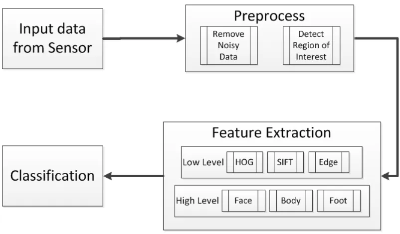
In this section, we review the major procedures for image recognition. A general image recog-nition method consists of three parts: image preprocess, feature extraction and classification.
1.1.1
Preprocess
Firstly, the optical property of an object is captured through its optical sensor of a digital camera and then the digital camera generates raw digital data of the image. After receiving the raw data of a image from the sensor, preprocess is to generate a new image from the source image. This new image is similar to the source image, but differs from it considering certain apsects, e.g. the new image has smoother edge, better contrast and less noise. Here, somepixel operations andlocal operationsare used to improve the contrast and remove the noise.
Figure 1.1: Major procedure for image recognition.
object appear in the central of the image and remove those irrelevant area.
The result of preprocess has great impact on the final result of the recognition. Clear and noise free images can make the feature extraction more effective and significantly improve the final classification accuracy.
1.1.2
Feature Extraction
Feature extraction is used to extract the optical properties of an image and represent interesting parts of an image from the raw image data as a compact feature vector. The feature vector is then used for either training the classifier or recognition. Therefore, feature extraction is the most important part for image recognition. The quality of the features extracted from a image have great impact on the recognition result. There are two major streams for feature extraction: the hand engineered method and representation learning method.
1.1.2.1 Hand Engineered Feature
[26], Scale Invariant Feature Transform (SIFT) [70], Speeded Up Robust Features (SURF) [8], Local Binary Patterns (LBP) [78], and color histograms [13]. Feature descriptors obtain from these low level features refer to a pattern or distinct structure found in an image, such as a point, the edges, or some small image patches. They are usually associated with an image patch that differs from its immediate surroundings by texture, color, or intensity. What the feature actually represents does not matter. We know that it is distinct from its surroundings. These low level
Figure 1.2: Feature extraction using SIFT.
features can be used directly for recognition. However, since they just represent certain local properties of an image and are not discriminative enough for recognition, discriminative high level features can be further learned by combining the low level features using some algorithms such as bag-of-visual words[62].
1.1.2.2 Representation Learning
Representation learning is mainly described by Deep Learning algorithms[58] or Auto En-coders [11]. The ideas is to learn a group of filters that are able to capture various kinds of features to discern one category of images from the another category with some supervised or unsupervised algorithm. Typically in representation learning, features are learned hierarchi-cally from low-level features to high level ones automatihierarchi-cally. Learning representation from an image can start from either low level hand-crafted features (for Auto Encoders) or raw pixels of an image (for Deep Learning).
Auto Encodersare widely used to combine different types of low level feature. The outputs
Figure 1.3: General Scheme of Auto Encoders. L1 is the input layer, possibly raw-pixel inten-sities. L2 is the compressed learned latent representation and L3 is the reconstruction of the given L1 layer from L2 layer. AutoEncoders tries to minimize the difference between L1 and L3 layers with some sparsity constraint.
level representations from Auto Encoders are learned by minimizing the reconstruction errors, they are still not robust enough to handle all kinds of variance of the objects in some tasks.
Deep Learning is the most popular approach for learning representations. It has been
widely used for all kinds of image recognition tasks and achieved the state-of-the-art perfor-mance on some large scale image recognition tasks, such as ILSVRC and The PASCAL Visual Object Classes Challenge (PASCAL VOC). Convolutional Neural Networks (CNN) is the most popular deep learning model for the image recognition tasks1. The first deep CNN that had great success on image recognition is the LeNet proposed by Y.LeCun in 1989 [64]. Back-propagation was applied to Convolutional Neural networks with adaptive connections. This combination, incorporating with Max-Pooling and speeding up on graphics cards has become an important part for many modern, competition-winning, feedforward, visual Deep Learners. Deep CNNs have been widely used as the feature extractor for all kinds of images recognition tasks and proven to be the most powerful method of feature extraction.
1Deep CNNs are sometimes considered as the end-to-end classifier while learning the feature representation
Figure 1.4: The architecture of ALEXNET (adopted from [58]).
1.1.3
Classification
After extracting feature representation from the images, a classifier is used to train a recogni-tion model as well as for predicting the new coming images. A supervised model is always used for training the recognition model. Discriminative Classifier such as Support Vector Ma-chine (SVM) is widely used as the classifier for recognition [24]. As we mentioned before, in order to capture different variances of the images for one category, the size of the feature representation for an image is usually very large. In order to avoid overfitting, the size of the training set should be at least the same size of the feature representation as well. Some classi-fiers such as Bayesian method or decision tree require to consider the correlations between each feature and the class labels and suffer from the large feature dimension. However, Discrimi-native Models[15] are more convenient for training. Discriminative Models can be effectively optimized with stochastic gradient descent and are suitable for the large training set.
However, to capture all variance of an object, training a good recognition model requires abundant data when we learn a model from scratch. With the limited training data, it is difficult to achieve a good classification performance. Transfer learning is an effective way to solve this problem by utilizing the knowledge from previous tasks. In this thesis, we focus on how to transfer the knowledge from the source domain for recognition tasks. The methods proposed in chapter3and chapter4mainly focus on the stage of classification while the method in chapter
Figure 1.5: An intuitive description for human to learn new concept: an okapi can be roughly described as the combination of a body of a horse, legs of the zebra and a head of giraffe.
1.2
Approaches in Visual Transfer Learning and the
Limi-tations
Previous work of visual transfer learning focuses on designing classifiers that can leverage the source knowledge effectively. In this section, we briefly review methods for the visual transfer learning and show the limitation of previous work.
1.2.1
Intuition for Visual Transfer Learning
The intuition of visual transfer learning comes from human recognition mechanism. For our human, all the information acquired is stored in our memory. This information is organized according to the properties. When we see a new concept, we don’t treat it isolated but connect it to certain previous knowledge we stored in our memory. By comparing a new concept with the organized information in our memory, we can capture the property of a new concept effectively. When referring to visual tasks, several examples can be given to show this cognitive ability. For instance, when we describe the animal ”okapi” (see Figure 1.5), we would probably say that: okapi has a body of a horse, legs of the zebra and the head of giraffe. People who never see a zebra could instantly have a rough idea of a zebra.
as transfer learning[79]. Traditional machine learning methods work under the common as-sumption: training data and testing data are drawn from the same feature space and same distribution. In transfer learning, the test data can come from a different distribution. The data from the original distribution is called source data, and data from the new distribution is called target data. Transfer learning is used to utilize the source knowledge from the source data to help to build the new model to classify the target data.
1.2.2
Approaches for Visual Transfer Learning
Successfully leveraging the source knowledge can greatly improve the performance of the tar-get model. In general, the more related the source and tartar-get domain are, the more useful the source knowledge is and the more benefit the target model can get. Leveraging unrelated knowledge cannot help to improve the performance of the target model or even hurt it. There-fore, the key issue for visual transfer learning is to identify the relatedness of the source and target domain. The major approach for Visual Transfer Learning consists of two main direc-tions: Distribution Similarity Measurement and Instance Reuse.
• Distribution Similarity Measurement. The core idea of transfer learning is to
lever-age the related source knowledge. The more related the source is, the better transfer performance we can achieve. Thus, measuring the relatedness of the source knowledge is an important part in transfer learning especially where there are multiple sources. A straight-forward approach to identify the relatedness of the source and target domain is to measure their similarity directly. Measuring the data discrepancy through some sta-tistical measurements such asMaximum Mean Discrepancy (MMD) [31], has been a
popular way to identify the source and target domain. MMD reflects the distance of two data distributions in the Reproducing Kernel Hilbert Space (RKHS) [3].
• Instance Reuse[67]. We apply transfer learning under the scenario where the target data
is scarce and we are not able to build the target model alone with the target data. A simple solution is to “borrow” some of the data from the source domain and use it to build the target model together with the target data. This approach can directly increase the size of the data in the target domain and effectively improve the performance of the target model. For example, Feature Transformation[32] can overcome the data distribution
Figure 1.6: Feature transformation. Transform the data in different domains into a augmented feature space.
1.2.3
Limitation of Previous Methods
From the review of the approaches for Visual Transfer Learning we can see that most previous methods require access to the source data to obtain the source knowledge. However, in many practical problems, these previous approaches may not be as convenient as we thought due to the following reasons:
• Data accessibility. The source data may not be able to access for some tasks. For
example, the clinical database is not allowed to access for general publics due to the privacy. Disclosure obligations and will to share the databases are also two important reasons that make the source data inaccessible.
• Size of the source data. Besides data accessibility, many previous methods [27][32]
re-quire accessing to each of the individual source instance to obtain the source knowledge which is ineffective for many large source domain. For example, it is almost impos-sible to measure the MMD for some large source domain which contains hundreds of thousands of instances.
From above we can see that these previous methods can successfully leverage the source knowledge under the assumption that the source data are freely accessible and relatively small. However, this assumption could fail in real applications. In some cases, the source data could be private (such as the clinic data from patients) and therefore, could not be shared with the public. Moreover, those large source dataset contains more knowledge and information com-pared to the small ones and thus can better improve the transfer performance of the target task. However, obtaining the similarity measurement of these large datasets with those previ-ous methods can be tediprevi-ous and inefficient. It is important to find a way to leverage the source knowledge without accessing to the source data.
for transfer learning can successfully avoid the two issues discussed above. Source model can contain as much knowledge as the source data while without containing any information regarding the individual instance. Therefore, the owner of the source data does not have to worry about the data privacy issue. For those large source dataset such as ILSVRC containing millions of images, a trained source model is normally a few hundreds megabytes and public available. Therefore, leveraging the source knowledge from source model instead of the source data is more practical for real visual transfer learning applications.
1.3
Main Contribution
In this section, we discuss the challenges that we may encounter when we can only access the source model. Then we demonstrate the learning scenarios and proposed solutions in this thesis.
1.3.1
Challenges
Despite for the general challenges in transfer learning, in our HTL settings, there are some new challenges in this thesis.
The first challenge isknowledge representation, i.e. how to obtain the source knowledge
when we are not able to access to the source data. When source data is accessible, the source knowledge is relatively explicit and we can easily obtain the source knowledge by either an-alyzing the source data distribution or make use of the source data to help training the target mode. The knowledge of the source domain is implicit and encoded in the source model using certain learning algorithms. How to effectively extract the source knowledge from the models is challenging.
The second challenge isknowledge expressiveness, i.e. how to leverage the source
knowl-edge to help training the target model. As the source knowlknowl-edge is implicit, how to effectively leverage the source knowledge and improve the transfer performance is also important. We also expect that the source knowledge extracted from the source model should be as general as possible so that the source knowledge can be extracted from different types of source model. Therefore, our transfer learning algorithm can work in many situations.
The last challenge is knowledge regularization i.e. how to guarantee the performance
Negative transfer [79] happens when the performance of target model degrades after receiving the knowledge from the source domain and how to avoid negative transfer is still an open question to all transfer learning researchers. The absence of the source data makes the situation more complicated.
1.3.2
Two Transfer Learning Scenarios
In this thesis, we mainly focus on two transfer learning scenarios: inductive transfer learning for new classes and domain adaptation. The definition of the two scenarios is as follows:
Definition Domain Adaptation[9] LetXbe the input space andY be output space. Given the source domain Ds and the target learning taskDt with marginal distribution P(Xs) and P(Xt),
we assume thatDsandDtshare the same conditional distributionP(Y|X). The goal of Domain
Adaptation is to learn theP(Xt|Yt) for the target task with the help ofDs.
Definition Inductive Transfer Learning[79] Given a source domainDsand the source
learn-ing taskTs, a target domianDt and the target learning taskDt, inductive transfer learning aims
to help improve the learning of the target task function ft(·) inDtusing the knowledge fromDs
whereDs , Dt.
The major difference between the two transfer learning scenarios is that in inductive transfer learning, the source and target tasks are two different but related tasks (e.g. from sport car to heavy truck) while in domain adaptation, the source and target tasks are the same task but with different marginal distributions (e.g. from the animation dog to the real dog).
(a) Domain Adaptation (b) Inductive transfer learning the new class
1.3.3
Proposed Methods
There are three methods proposed in this thesis, one in inductive transfer learning for new classes and two methods in domain adaptation.
In chapter 3, we extend the previous methods in HTL which are limited to using SVMs as the source model and propose a novel method Effective Multi-class Transfer Learning
(EMTLe) for supervised domain adaptation. We use the output of the source model as the auxiliary bias to adjust the target model. Here, the output of the source model is used as the prior to adjust the decision for the target model. As long as we can set a proper weight to the prior knowledge, the source model can serve well for the target task. Because we only require the source model to provide its decision, we can treat it as a black-box model and EMTLe can leverage the source model from any source classifier that can generate the class probability of an example.
In chapter4, we investigate the problem of semi-supervised domain adaptation where most of the data in the target task are unlabeled and propose a novel frameworkGeneralized Distil-lation Semi-supervised Domain Adaptation (GDSDA). In GDSDA, the source model
gen-erates “soft labels” for the target data and can improve the performance together with the true labels from target task. We use the imitation parameter to determine the relative importance of the soft label and true label. Then we propose GDSDA-SVM that can determine the imitation parameter autonomously through cross-validation.
In chapter5, we use the deep neural network to solve the transfer learning problem for food recognition. We use GoogLeNet trained from ImageNet of 1000 classes as our source model and two food databases as our target task, containing 101 classes and 265 classes respectively. In this chapter, we don’t treat the source model as a black-box. Instead, we can obtain the parameters of the original GoogLeNet. We re-use the parameters in the original GoogLeNet as the prior and fine-tune it on our target task to achieve the improved performance. By re-using and fine-tuning the parameter, i.e. features from source tasks, we can effectively learn new categories of the target task. We show that without accessing the source data, we can still achieve better performance compared to previous methods.
1.4
Summary
Related Work
In this chapter, we review some previous work related to ours. We first review the classifiers used in this thesis, providing the general concept and principle of how they work. Then we review the types of transfer learning for visual recognition from two different views and then discuss the previous work of how to alleviate negative transfer. Finally, we review some meth-ods related to the three methmeth-ods used in this thesis.
2.1
Classifiers for Image Recognition
In our scenario, we have to face the problem of image recognition. Due to the large dimension of the feature representation for each image as well as the size of training image, manual classification is hopeless. As we mentioned in Section 1.1, a recognition model is used to distinguish the objects from different categories automatically trained by supervised learning. In this section, we introduce the classifiers we used in this thesis.
2.1.1
Binary Classification and Multi-class Classification
In image recognition, we train a recognition model from a set of training images along with their labels provided. The labels are predefined in a category space. Thus, the task of image recognition is to classify each image as one predefined category. If there are only two cate-gories, this recognition task is called binary classification. For the task recognizing the objects from more than two categories, the recognition task is called multi-class classification [4] [58]. Here, we give a formal definition of the scenario for binary and multi-class classification. Generally, we can decompose the multi-class learning task into a set of binary scenarios by training a binary classifier for each class, e.g. One-VS-Rest strategy (see figure2.1)[82] [102].
Figure 2.1: One-vs-Rest strategy for multi-class scenario. A three classes problem can be decomposed into 3 binary classification sub-problems.
The binary scenario for classification can be defined as follow: given a dataset from domain
X × YwhereXis the input feature representation andYis the binary label set{1,−1}(for some
classifier,{1,0}is also used). We usually use the label 1 to denote the examples belong to one
certain category and -1 to denote examples not belong to that category. We assume that the training image setDtrain ={(xi,yi)} ⊂ X × Yand the test image setDtest = {(xti,yti)} ⊂ X × Yare
given and separated from each other. Each pair (xi,yi) denotes the input feature representation
xiand its corresponding labelyifor theithimage in the both set. Our goal of the classification
problem is to learn a decision function f : X → Yfrom the training setDtrainsuch that f can
achieve good performance on bothDtrainandDtest.
2.1.2
Softmax Classifier
In this subsection, we will introduce a widely used linear classifierSoftmax classifierin image
into the class scores and the loss function that quantifies the agreement between the predicted scores and the ground truth labels. Linear classifier often works very well when the number of dimensions of the input is large. Therefore, it is widely used as the classifier for image recognition, especially as the classifier for Convolutional Nueral Networks [64].
Typically, Softmax classifier is widely used for multi-class image classification. Softmax classifier (also called multinomial logistic regression) is a generational form of logistic regres-sion for the multi-class scenario. As logistic regresregres-sion can only handle the binary classification scenario, Softmax classifier adapts the one-vs-rest strategy where several logistic regression models are trained for each class.
Given a training set {(x1,y1),(x2,y2), ...,(xm,ym)}, we assume the label yi ∈ {1,0}and the
input feature xi ∈ Rn. For each binary logistic regression model, The score function takes the
form:
fw(x)=
1
1+exp(−wTx) (2.1)
and the parametersware optimized to minimize the following loss function:
l(w)=−[ m
X
i=1
yilog fw(xi)+(1−yi) log(1− fw(xi))] (2.2)
For Softmax classifier, it is used to handle the multi-class classification problem and sup-pose there are N classes. Therefore,ycan take from N different values{1,2,3, ...,N}instead
of just two. For a given test example x, the score function estimate the probability P(y = n|x)
for each value ofn= 1,2,3, ...,N, i.e. estimate the probability that each score assigns the input xto the N classes associated to the N different possible values. Thus, the score function will output a N-dimensional vector providingN estimated probabilities whose sum of elements is 1. TheN dimensional output of the score function can be generated according to the following form:
fw(x)=
P(y=1|x;w)
P(y=2|x;w)
...
P(y=n|x;w)
= PN 1
j=1exp w(j)Tx
exp
w(1)Tx exp
w(2)Tx
...
exp
w(N)Tx
(2.3)
Herew(1)T,w(2)T, ...,w(N)T are the parameters of the Softmax classifier model. The term 1
PN
j=1exp(w(j)Tx)
is called the normalization term so that theN distributions sum to 1.
To optimize the parameters w(1)T,w(2)T, ...,w(N)T, the cross-entropy loss used for the Soft-max classifier is defined as:
J(w)=−
l X
i=1 N
X
k=1
`{yi =k}log
exp
w(k)Tx i
PN
j=1exp w(j)Txi
Here`xis the 0-1 loss function:
`{x}=
1 xis true
0 xis false (2.5)
It is noted that Eq (2.4) is a generalized form of Eq (2.2). Minimizing Eq (2.4) can be inter-preted as minimizing the negative log likelihood of the correct class, which is equivalent to performing Maximum Likelihood Estimation (MLE) [53].
The minimum of J(w) can be obtained by gradient descent method while taking the gradi-ent:
∇J(w(n))= − l
X
i=1
xi
`{yi = n} −
exp
w(k)Tx i
PN
j=1exp w(j)Txi
(2.6)
2.1.3
Support Vector Machines
In this subsection, we will review another widely used discriminant classifier,Support Vector Machine(SVM) [24]. SVM is another classifier that has been adoptive in many image
recog-nition tasks [22] [89] [110]. In this thesis, we also use a classifier based on SVM. We will give a detailed description of SVM.
As we mentioned before, the linear classifier consists of two parts: the score function and loss function. SVM classifier can be divided into two categories based on their score function: linear SVM that uses a linear discriminant function and kernel SVM that uses kernel function. Kernel SVM can be considered as a extension version of linear SVM where kernels are used for calculate the scores of the inputs. Another difference for between linear and kernel SVM is linear SVM can be solved on the primal problem while kernel SVM is mostly optimized on its dual [24] [90].
First, we will introduce the linear SVM. Linear SVM uses the simplest representation of a score function by taking the linear combination of the input vector:
f(x)= wTx+b (2.7)
where w is called the weight vector and b is called the bias. In a binary scenario, for the input example x and the class labels y ∈ {c1,c2}, x is assigned to class c1 if f(x) ≥ 0 and
c2 otherwise. Therefore, the corresponding decision surface is defined by f(x) = 0. For two points x1 and x2 lie on the decision surface, we have f(x1) = f(x2) = 0. Then we can have
wT(x
1− x2) = 0 and hence the weight vector wis orthogonal to every point lying within the
decision surface, i.ewdetermines the orientation of the decision surface. Similarly, ifxlies on the decision surface, the normal distance from the origin to the decision surface is given by:
wTx
||w|| =−
b
(a) Different sparating hyperplanes (b) Max-Margin hyperplanes
Figure 2.2: Support Vector Machine
Therefore, we can see that, the location of the decision surface is determined by the biasb.
2.1.3.1 Hard Margin SVM
Hard margin SVM is used to find the optimal solution for the data sets that are linear separable. Given a set of n training points (x1,y1),(x2,y2), ...,(xn,yn) where yi ∈ {1,−1}, we expect to
find a decision surface that can separate the data from two classes. However, when the data from these two classes can be linearly separated, there could be several decision surfaces that can separate the data. The idea of SVM is to choose the maximal margin decision surface so that the distance between these two classes is as large as possible (called maximal margin hyperplane). For example, in figure2.2(a),H2 andH3 are two candidate decision surface that can separate the data. However, H3 is has the largest distance to all the data from two classes and SVM will chooseH3 as the optimal hyperplane.
The optimal hyperplane can be found by minimizing the following objective function:
min ||w||2
s.t. yi(wTxi+b)≥1 for all 1≤i≤ n
(2.9)
2.1.3.2 Soft Margin SVM
In real world application, most data are not linear separable. Therefore, SVM introduce the concept of slack variable to handle this situation. Slack variable is defined as:
Figure 2.3: Slack variables for soft-margin SVM
The value of slack variable is 0 if the example xi lies on the correct side of the margin. For
those data on the wrong side, its value is proportional to the distance from the correct margin. Therefore, to find the parameters of hyperplane, i.e. weight vectorwand biasb, soft-margin SVM minimize the following loss function:
min λ
2||w||2+ 1 n
n
X
i
ξi
s.t. yi(wTxi+b)≥1−ξi
ξi ≥0 for all 1≤i≤ n
(2.11)
The objective function is called primal of SVM. A stochastic sub-gradient descent can be used to find the optimal solution for eq. (2.11) effectively [90].
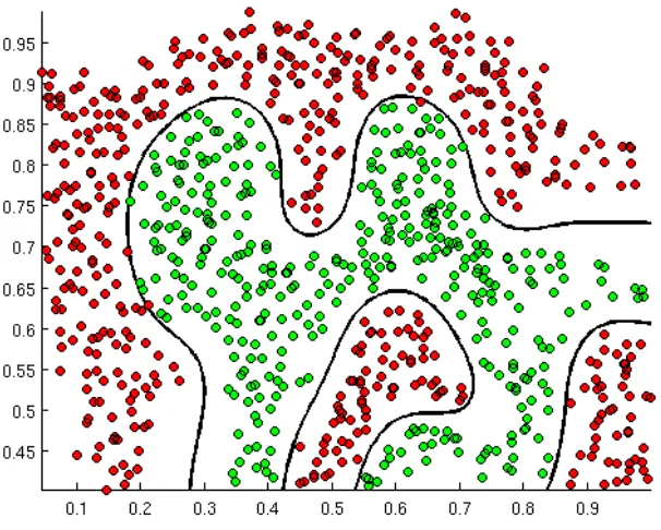
2.1.3.3 Kernel SVM
Linear soft-margin SVM works well when number of features is larger than number of training examples. However, when the size of the training example is larger than the features, kernel SVM (such as Gaussian Kernel) with proper parameters outperforms linear SVM [56].
Figure 2.4: The hyperplane of SVM with RBF kernel for non-linear separable data.
find the optimal hyperplane in the high-dimensional feature spaces. Given a feature space mappingφ(x), the score function for kernel SVM can be re-written as:
f(x)= wTφ(x)+b (2.12)
From eq (2.12) we can see that, when we take the identity mappingφ(x)= x, the kernel SVM becomes a linear SVM. Therefore, the linear SVM can be considered as a special case of kernel SVM where identity mapping is used as the kernel. The loss function of kernel SVM is almost identical to eq. (2.11) except for replacing the term xwithφ(x):
min λ
2||w||2+ 1 n
n
X
i
ξi
s.t. yi(wTφ(x)i+b)≥1−ξi
ξi ≥0 for all 1≤i≤ n
(2.13)
the dual of kernel SVM function:
max
n
X
i
αi− n
X
i n
X
j
yiyjαiαjφ(xi)φ(xj)
s.t. 0≤αi ≤
1
λ
n
X
i
yiαi =0 for all 1≤i≤ n
(2.14)
We can obtain the solution of (2.14) by Sequential Minimal Optimization (SMO) [81] or Dual Coordinate Descent [46].
There are several advantages of using SVM as the classifier:
• Generalization ability. SVM provides good generalization ability by maximizing the
margin between the examples of the two classes. By setting the proper parameters and generalization grade, SVM can overcome some bias from the training set. Therefore, SVM is able to make correct prediction for unseen data. This ability can be very useful for image recognition as there is no image dataset that can cover all the transformation of the objects. Moreover,the idea of soft-margin makes it robust against noisy data.
• Kernel transformation.By introducing the non-linear transformation of the input, SVM
can model complex non-linear distributed data. The kernel trick can greatly improve the computational efficiency.
• Unique solution.The objective function of SVM is convex. Compared to other methods,
such as Neural Networks, which are non-convex and have many local minima, SVM can deliver a unique solution for any given training set and can be solved with efficient methods, like sub-SGD [90] or SMO [81].
2.1.4
Convolutional Neural Networks
Convolutional Neural Networks [65] is the most popular and powerful method for image recog-nition task. In this part, we introduce the history of Convolutional Neural Networks. The detail description of the Convolutional Neural Networks layers will be included in chapter5.
2.1.4.1 Early Work with Convolutional Neural Networks
could be the first DL systems of the Feedforward Multilayer Perceptron type [48][88]. Later, there have been many applications of GMDH-style nets [38] [47] [57] [108].
Apart from deep GMDH networks, the Neocognitron, a hierarchical, multilayered artifi-cial neural network, was perhaps the first artifiartifi-cial NN to incorporate the neurophysiological insights [40]. Inspired by Neocognitron, Convolutional NNs (CNNs) was proposed where the rectangular receptive field of a convolutional unit with given weight vector is shifted step by step across a 2-dimensional array of input values, such as the pixels of an image (usually there are several such filters). The results of the previous unit can provide inputs to higher-level units, and so on. Because of its massive weight replication, relatively few parameters may be necessary to describe its behavior.
In 1989, backpropagation [64][65] was applied to Convolutional Neural networks with adaptive connections [64]. This combination, incorporating with Max-Pooling and speeding up on graphics cards has become an important part for many modern, competition-winning, feedforward, visual Deep Learners. Later, CNNs achieved good performance on many practical tasks such as MNIST and fingerprint recognition and was commercially used in these fields in 1990s [7] [63].
In the early 2000s, even though GPU-MPCNNs wons several official contests, many prac-tical and commercial pattern recognition applications were dominated by non-neural machine learning methods such as Support Vector Machines (SVMs).
2.1.4.2 Recent Achievements with Convolutional Neural Networks
In 2006, CNN trained with backpropagation set a new MNIST record of 0.39% without us-ing unsupervised pre-trainus-ing [75]. Also in 2006, an early GPU-based CNN implementation was introduced which was up to 4 times faster than CPU-CNNs [20]. Since then, GPUs or graphics cards have become more and more essential for CNNs in recent years. In 2012, a GPU implemented Max-Pooling CNNs (GPU-MPCNNs) was also the first method to achieve human-competitive performance (around 0.2%) on MNIST [21].
Fer-gus improve AlexNet by 1.7% on top 5 accuracy [115]. By both adding extra convolutional layers between two pooling layers and reducing the receptive field size, Simonyan and Zis-serman built a 19 layer very deep CNN and achieved 92.5% top-5 accuracy [92]. After the AlexNet-like deep CNNs won ILSVRC2012 and ILSVRC2013, Szegedy et al. built a 22-layer deep network, called GoogLeNet and won the 1st prize on ILSVRC2014 for 93.33% top-5 accuracy, almost as good as human annotation[96]. Different from AlexNet-like architecture, GoogLeNet shows another trend of design, utilizing many 1×1 receptive field. Recently, Wu et.
al present an image recognition system by aggressive data augmentation on the training data, achieving a top-5 error rate of 5.33% on ImageNet dataset[109]. Searchers from Google suc-cessfully trained an ingredient detector system based on GoogLeNet with 220 million images harvested from Google Images and Flickr [74].
Besides its impressive performance on those huge datasets, MPCNNs shows some impres-sive results by fine-tuning the existing models on small datasets.Zeiler et al. applied their pre-trained model on Caltech-256 with just 15 instances per class and improved the previous state-of-the-art in which about 60 instances were used, by almost 10% [115]. Chatfield et al. used their pre-trained model on VOC2007 dataset and outperformed the previous state-of-the-art by 0.9% [19]. Zhou et al. trained AlexNet for Scene Recognition across two datasets with identical categories and provided the state-of-the-art performance using our deep features on all the current scene benchmarks [116]. Hoffman et al. fine-tuned the MPCNNs trained from Im-ageNet with one example per class, showing that it is possible to use a hybrid approach where one uses different feature representations for the various domains and produces a combined adapted model [45].
To summarize, in this section, we have briefly reviewed three types of classifier for image recognition, namely Softmax classifier, SVM and CNNs. Softmax classifier is typically used as the last layer of CNNs. Linear SVM is a general method for the image recognition. Moreover, The generalization ability of SVM classifier can reduce the bias from the training data.
2.2
An Overview of Visual Transfer Learning
Traditional machine learning algorithms try to build the classifiers from a set of training data and apply to the test data with the same distribution to the training data. In contrast, transfer learning attempts to change this by transfer the learned knowledge from one or several tasks (called source tasks) to improve a related new task (called target task). According to the
Figure 2.5: Apart from the standard machine learning, transfer learning can leverage the infor-mation from an additional source: knoweldge from one or more related tasks.
instance transfer, feature representation transfer and parameter transfer.
Table 2.1: Categories of our learning scenarios
Situation of Task Source Knowledge Learning New Categories Inductive Transfer
Parameter Transfer Domain Adaptation Transductive Transfer
2.2.1
Types of Transfer Learning from the Situations of Tasks
Transfer learning can be categorized into 3 sub-settings: inductive transfer learning, trans-ductive transfer learningand unsupervised transfer learningbased on the different
situa-tions of the source and target domains and tasks. [79]. We compared the differences of these three sub-categories and show them in Table2.3.
Table 2.2: Relationship between traditional machine learning and different transfer learning settings
Learning settings Source target domain Source target task
Traditional machine learning the same the same
Transfer learning
Inductive transfer learning the same different but related
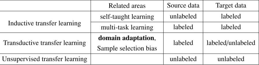
Table 2.3: Various settings of transfer learning
Related areas Source data Target data
Inductive transfer learning self-taught learningmulti-task learning unlabeledlabeled labeledlabeled
Transductive transfer learning domain adaptation,
Sample selection bias labeled labeled/unlabeled
Unsupervised transfer learning unlabeled unlabeled
2.2.2
Types of Transfer Learning from the Aspect of Source Knowledge
According to the type of the source knowledge comes from, transfer learning can be split into 3 major streams: instance transfer, feature representation transfer and parameter transfer.
The core idea of instance transfer learning is to select some useful data from the source task to help learning the target task. Dai et al. [25] propose a method (called TrAdaBoost) that can select the most useful examples from the source task as the additional training examples for the target task. These useful examples are iteratively re-weighted according to the classification results of some base classifiers. Jiang et al. [51] proposed a method that can ignore the ”mis-leading” examples from the source data based on the conditional probabilities on the source task P(yt|xt) and target task P(ys|xs). Liao et al. [66] proposed a active learning method that
selects and labels the unlabeled data from the target data with the help of the source data. Ben-David et al. [9] provided a theoretical analysis the lowest target test error for different source data combination strategies when the source data is large and target training set is small.
Feature representation transfer aims to find a good feature representations to reduce the gap between the source and target domains. According to the size of labeled examples in the source data, feature representation transfer consists of two approaches: supervised feature con-struction and unsupervised feature concon-struction. When the source data are labeled, supervised feature transfer learning is used to find the feature representations shared in related tasks to reduce the difference between the source and target tasks. Evgeniou et al. [34] proposed a method that can learn sparse low-dimension feature representations that can share between dif-ferent tasks. Jie et al. [52] reconstructed the feature representations for the target data by using the outputs of the source models as the auxiliary feature representations. In unsupervised fea-ture representation transfer learning, Daume III [27] proposed a simple feature reconstruction method for both source and target data so that source and target data are triple augmented and a SVM model is trained on both source and target data.
Figure 2.6: Two steps for parameter transfer learning. In the first step multi-source and single source combination are usually used to generate the regularization term. The hyperplane for the transfer model can be obtained by either minimizing training error or cross-validation error on the target training data.
the hyperparameters in the individual models of related tasks. Most of the approaches are designed under the multi-task learning scenario. Therefore, in this thesis, we also focus on the parameter transfer approach to leverage the knowledge from the source data. In parameter transfer learning, there are three major frameworks: a regularization framework, a Bayesian framework and a neural network framework.
• Regularization framework: In the regularization framework, some researchers propose
to transfer the parameters of the SVM following the assumption that the hyperplane for the target task should be related to the hyperplane of the source models. Evgeniou et al. [35] proposed an idea that the hyperplane of the SVM for the target task should be separate into two terms: a common term shared over tasks and a specific term related to the individual task. Inspired by this idea, some researchers propose different strategies to combine these two terms for transfer learning [4] [98] [112]. Most of these work contains two steps. In the first step, a SVM objective function with a biased regularization term for the target model is built. Then another objective function is built to reduce the empirical error of the target model on the target data.
• Neural network framework. In neural network framework, the idea is to use the
are more related to a specific task while the low level layer ones are more general and transferable. This framework is widely used for image recognition task. By re-using and fine-tuning the parameters of some layers in the pre-trained model, the bias of the target task can be greatly alleviated [19] [45] [115] [116].
• Bayesian framework. In Bayesian framework, one or several posterior probabilities of
the source data or parameters of the source model can be used to generate a prior proba-bility for the target task. With this prior probaproba-bility, a posterior probaproba-bility for the target task can be obtained with the target data. Li et al. [39] used a prior probability density function to model the knowledge from the source and modify it with the data from target to generate posterior density for detection and recognition. Rosenstein et al. [87] used hierarchical Bayesian method to estimate the posterior distribution for all the parameters and the overall model can decide the similarities of the source and target tasks.
2.2.3
Special Issues in Avoiding Negative Transfer
In transfer learning, for a given target task, the performance of a transfer method depends on two aspects: the quality of the source task and the transfer ability of the transfer algorithm. The quality of the source task refers to how the source and target tasks are related. If there exists a strong relationship between the source and target, with a proper transfer method, the performance in the target task can be significantly improved. However, if the source and target tasks are not sufficiently related, despite of the transfer ability of the transfer algorithm, the performance in the target task may fail to be improved or even decrease. In transfer learning, negative transfer refers to the degraded performance compare to a method without using any knowledge from the source [79]. How to avoid negative transfer is still an open question for researchers. For example, we can use a teacher-student diagram to illustrate the procedure of transfer learning. The student (target model) would like to learn the new knowledge (target task) with the assistance of a teacher (source knowledge). If the teacher can provide helpful knowledge (related knowledge), the student can learn the new knowledge very quickly (positive transfer). If the teacher can only provide useless knowledge, the student could not learn the new knowledge effectively or even get confused (negative transfer).
Figure 2.7: Positive transfer VS Negative transfer.
negative transfer [100]. Even though voiding negative transfer is an important issue in transfer learning, how to avoid negative transfer has not been widely addressed [71] [79]. Previous work show suggest that negative transfer can be alleviated through 3 approaches [100]:
• Rejecting unrelated source information. A important approach to avoid negative
trans-fer is to recognize and reject unrelated and harmful source knowledge. The goal of this approach is to minimize the impact of the unrelated source, so that the transfer model performs no worse than the learned model without transfer. Therefore, in some extreme situation, the transfer model is allowed to completely ignore the source knowledge. Tor-rey et al. [101] proposed a method using advice-taking algorithm to reject the unrelated source knowledge. Rosenstein et al. [87] presented an approach that use naive Bayes classifier to detect and reject the unrelated source.
• Choosing correct source task. When the source knowledge come from more than one
candidate source, it is possible for the transfer model to select the best source knowledge of the candidates. In this scenario, leverage the knowledge from the best candidate may be effective against negative transfer as long as the best source knowledge is sufficiently related. Talvitie et al. [97] proposed a method that can iteratively evaluate the candidate sources through a trail-and-error approach and select the best one to transfer. Kuhlmann et al. [59] constructed a kernel function from certain sources for the target task by esti-mating the bias from a set of candidate sources whose relationship to the target task is unknown.
• Measuring task similarity. To achieve a better transfer performance, it is reasonable for a
a single source. In this approach, some methods try to involve all the source knowledge without considering the explicit relationship between the source and target. The other methods try to model the relationships between the source and target tasks and use the information as a part of their transfer methods which can significantly reduce the af-fect of negative transfer. Bakker et al. [6] proposed a method to provide guidance on how to avoid negative transfer by using clustering and Bayesian approach to estimate the similarities between the target task and multiple source tasks. Tommasi et al. [99] constructed the transfer model by using some transfer parameters to measure the relation-ships between each source and the target tasks and the transfer parameters are optimized by minimizing the cross-validation error of the transfer model. Similar approaches can be found in [52] [61]. Kuzborskij et al. [60] provided some theoretical analysis of trans-fer learning and show that regularized least square SVM with truncation function and leave-one-out cross-validation for source task measurement can reduce negative transfer even though the training data of the target task is relatively small.
Here we can see that most of the previous approaches focus on measuring the similarity of the source and target tasks, i.e. try to assign the most related source tasks to the target one through various of metrics and use aggressive transfer algorithm to exploit the source knowledge. Just a few work [60] [98] addressed the problem that a sophisticated transfer algorithm should be designed to better exploit the source knowledge as well as avoid negative transfer. Therefore, in this thesis, we mainly focus on how to design a better transfer algorithm for transfer learning while certain source knowledge is assigned.
To summarize, in this section, we provided an overview of the categories of transfer learn-ing from two different views. From the relationships of the tasks, our two transfer learnlearn-ing scenarios belong to inductive transfer and transductive transfer learning respectively. In this thesis, we assume that we are not able to access to the source data, therefore, from the as-pect of source knowledge, we use parameter transfer for both scenarios. In this thesis, without observing any source data, it is difficult to measure the relationship between the source and tar-get tasks. Therefore, avoiding negative transfer is also an important part we have to consider. Finally, we reviewed some methods that cab alleviate negative transfer.
2.3
Related Work in Hypothesis Transfer Learning
learning related to our work in chapter5. Then we discuss some methods in hypothesis transfer learning, which is related to our work in chapter3. The related work in chapter4is reviewed at last.
2.3.1
Fine-tuning the Deep Net
Since Deep Convolutional Neural Networks (CNNs) became the most powerful algorithm in object recognition task, fine-tuning the deep CNNs has become a popular and effective way to transfer the knowledge between different visual recognition tasks. The intuition of fine-tuning the deep CNNs for transfer learning is that low-level features, such as edges and lines, are universal for object recognition while high-level features, which are the combinations of the low-level features, are more specific for the designed task. Because deep CNNs can learn hierarchical features, from abstract low-level features to detailed high-level ones, by changing the combinations of the low-level features in the pre-trained deep CNNs, the high-level features can be learned effectively for the new recognition task [37].
Applying the pre-trained model from ImageNet dataset on other object recognition bench-mark datasets shows some impressive results. Zeiler et al. [115] applied their pre-trained model on Caltech-256 with just 15 instances per class and improved the previous state-of-the-art in which about 60 instances were used, by almost 10%. Chatfield et al. [19] used their pre-trained model on the VOC2007 dataset and outperformed the previous state-of-the-art by 0.9%. Agrawal et al. [1] show that even in the mid-level features, there are some grandmother cells, which can capture the high-level features of specific objects. Hoffman et al. [45] show that even with one labeled example per class, it is possible to fine-tune the pre-trained deep CNNs and obtain a good classifier for some new recognition tasks. Zhou et al. [116] provided the state-of-the-art performance using the deep features on some scene benchmarks by fine-tuning the deep CNNs. Yosinski et al. [114] investigated the transferability of the layers in deep CNNs and show that the target task can be benefited from pre-training even though the source and target tasks are distant.
In this thesis, we also use the pre-trained deep CNNs to learn new categories for food recognition and investigate the affects of each layer in deep CNNs for knowledge transfer in chapter5.
2.3.2
Hypothesis Transfer Learning with SVMs
In this part, We will introduce the framework ofHypothesis Transfer Learning(HTL). HTL
![Figure 1.4: The architecture of ALEXNET (adopted from [58]).](https://thumb-us.123doks.com/thumbv2/123dok_us/1949701.1256600/18.612.83.536.82.230/figure-architecture-alexnet-adopted.webp)