UCA-NW Algorithm for Space-Time Antijamming
Fulai Liu1, 2, *, Miao Zhang2, Xianchao Wang2, and Ruiyan Du1, 2
Abstract—Space-time antijamming problems cause widespread concern recently in global navigation satellite system. Space-time adaptive procession (STAP) is an effective method to suppress interference signals, which contains two adaptive filters, i.e., spatial filter and temporal filter, and the array pattern can be automatically optimized by adjusting the weights obtained from a prescribed objective function. However, mismatch may occur between adaptive weights and data, due to the change of the interference location when receiver is shaking. In this case, the performance of STAP will degrade dramatically. To solve this problem, an effective nulling widen method based on uniform circular array (named as UCA-NW algorithm) is proposed for space-time antijamming. Through this method, an extension matrix is given to modify the covariance matrix, and the formed null can be broadened from azimuth angle and pitch angle, respectively. Thus, this algorithm can suppress interference signals effectively when the receiver is shaking, and the width of nulls can be controlled easily. Simulation results are presented to verify the feasibility and effectiveness of the proposed algorithm.
1. INTRODUCTION
Global navigation satellite system (GNSS) is fully operational presently and provides accurate, continuous, three-dimensional position and velocity information to users with appropriate receiving equipment at any time [1]. However, due to the long distance between satellite and receiver, the power level of satellite signals is so weak that the performance of GNSS can be affected by various interference signals from either intentional or unintentional sources. Therefore, the performance of navigation and positioning might degrade dramatically [2]. Space-Time Adaptive Procession (STAP) is an effective technique to mitigate interference signals, which can not only enhance satellite signals in the presence of interference signals and noise but also suppress interference signals through an array of antennas. This technique is widely used in radar, sonar, wireless communication, radio astronomy, and many other fields [3]. In practice, due to the shake of receiver, the directions of arrival (DOA) of interference signals could change rapidly with time going on, which may cause the interference signals moving out of the narrow nulls formed by conventional space-time adaptive beamformers easily [4]. Thus conventional STAP algorithms are quite susceptible to the nonstationary interference signals, and the performance of conventional STAP algorithms may degrade seriously with the change of interference location.
In order to solve such problems, null-widen technique is presented to improve the performance of conventional STAP algorithms when the receiver is shaking. This technique can form a null with certain width at the location of the interference signals. Even if the receiver is shaking, the interference signals cannot move out of the formed null range. A null-widen method by adding virtual interference sources and constructing new covariance matrix is proposed by Mailloux [5]. Through expanding the bandwidth of interference signals, Zatman also gives a null-widen algorithm [6]. A concept of “Covariance Matrix Taper (CMT)” is proposed by Guerci through generalizing Mailloux’s method and Zatman’s method [7].
Received 14 June 2018, Accepted 23 July 2018, Scheduled 31 July 2018 * Corresponding author: Fulai Liu ([email protected]).
Combined with the CMT approach and adaptive variable diagonal loading technique, an approach for null broadening beamforming is proposed. This approach can improve the robustness of adaptive antenna null broadening beamforming when array calibration error exists [8]. The convex programming is used in [9] to optimize the covariance matrix. Through this method, the null can be broadened, and the sidelobe level can be controlled efficiently. Unfortunately, this method has a higher computational complexity. In [10], genetic algorithm is used to broaden nulls, but the depth of the null may be too low to suppress interference signals efficiently, and the output signal to interference plus noise ratio (SINR) could decrease dramatically. The space-time averaging technique and the rotation technique of the steering vectors are exploited in [11]. Through these two techniques, the presented algorithm can widen the width of nulls and provide increased robustness against the mismatch problem as well as control over the sidelobe level. In order to gain deeper nulls, a new method is proposed by reconstructing the interference-plus-noise covariance matrix to improve the performance of null level. This algorithm can get a deeper null although the receiver is shaking [12]. A robust beamforming control algorithm based on semidefinite programming is presented to broaden nulls of adaptive antenna array. In the actual system, this proposed approach is proved effectively through imposing broadened nulls on the interference region while possessing a well-maintained pattern [13]. A novel statistical null-widen method is proposed in [14]. Using this method, interference signals can be suppressed effectively, and the robustness of antijamming algorithm can be improved remarkably with limited array size under uniform linear array (ULA).
However, most of the null widening algorithms researched recently are used in spatial adaptive beamforming algorithms based on ULA. In order to improve the performance of the null widening algorithm and the freedom of antijamming, in this paper, a UCA-NW algorithm is proposed. By using the extension matrix, the formed null can be widened from azimuth angle and pitch angle, respectively, and the null level can be controlled easily. The rest of the paper is organized as follows. The data model is described in Section 2. Section 3 introduces the proposed method. Section 4 gives some simulation results. Finally, the conclusion is summarized in Section 5.
2. DATA MODEL
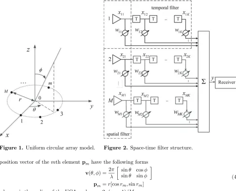
The geometric structure of a uniform circular array (UCA) with M elements is shown in Figure 1. Each element in the UCA is equally spaced with K taps, and the space-time filter structure is given in Figure 2.
The MK×1 space-time observation signal x(t) = [x11, x12, . . . , x1K, . . . , xMK]T can be expressed as
x(t) =us(t) + Q
q=1
gqjq(t) +n(t) (1)
wheres(t) denotes the desired satellite signal, andjq(t) denotes theqth interference signal. tis the index of time. n(t) represents the white Gaussian noise of antenna array. u and gq stand for the space-time steering vector of the desired satellite signal and the qth interference signal, which have the following forms
u=a(θ0, φ0)⊗at(T)
gq =a(θq(t), φq(t))⊗at(T) (2)
whereθ0 and φ0 are the azimuth angle and pitch angle of the desired satellite signal. θq and φq are the azimuth angle and pitch angle of the qth interference signal. a(θ, φ) andat(T) in (2) can be written as follows
a(θ, φ) =
e−jvT(θ,φ)p1, e−jvT(θ,φ)p2, . . . , e−jvT(θ,φ)pMT
at(T) =
1, e−j2πf0T, . . . , e−j2πf0(K−1)T
T (3)
Figure 1. Uniform circular array model. Figure 2. Space-time filter structure.
position vector of themth elementpm have the following forms
v(θ, φ) = 2π λ
sinθ cosφ sinθ sinφ
pm=r[cosrm,sinrm]
(4)
wherer is the radius of the UCA andrm = 2π(m−1)/M.
Thus, the beamformer output of the space-time filter can be expressed as
y(t) =wHx(t) (5)
where w= [w11, w12, . . . , w1K, . . . , wM1, . . . wMK]T is the MK×1 weight vector. The superscript (·)H denotes the conjugate transpose.
3. ALGORITHM FORMULATION
In order to suppress the interference signal, the DOA of theqth interference signal changing with time
can be described as
¯
θq=θq+ Δθq ¯
φq=φq+ Δφq (6)
whereθq andφq are azimuth angle and pitch angle of the qth interference signal. Δθqand Δφq are the changes of azimuth angle and pitch angle. Because the change of DOA is very small with high probability, suppose that Δθq obeys normal distribution with a mean of 0 and a variance of ξ2q1(Δθq ∼N(0, ξq21)), and Δφq obeys normal distribution with a mean of 0 and a variance of ξq22(Δφq ∼ N(0, ξq22)). The above model is used in [15] and [16] to describe the distributed targets and the transmit characteristics of mobile communication. Thus, the mean covariance matrix can be given by
¯
RL(m, n) = Q
q=1 σ2
q
f(Δθq,Δφq)e−j[pm−pn]Tv(¯θq,φ¯q)d(Δθ
where σ2q and σe2 denote the power of the qth interference signal and noise signal, respectively. f(Δθq,Δφq) stands for the joint probability density function of (Δθq,Δφq). δmn = 0 when m = n, and δmn = 1 when m=n. The vector v(θ, φ) and the position vector pm are given in Eq. (4). Thus, the vector v(¯θq,φ¯q) in Eq. (7) can be expressed as
v θ¯q,φ¯q=v(θq+ Δθq, φq+ Δφq). (8) Owing to the extension angle Δθq and Δφq are statically independent of each other. Thus, the vector v(θq+ Δθq, φq+ Δφq) in (8) can be simplified by Taylor series, and ¯RL(m, n) can be written as
¯
RL(m, n)≈ Q
q=1 σ2
qe−j 2π
λ[pm−pn]Tv(θq,φq)AmnBmn+σ2
eδmn (9)
whereAmn andBmn in Eq. (9) can be expressed as
Amn=
f(Δθq)e
−j2π
λ[pm−pn]T
cosθqcosφq cosθqsinθq
Δθq
d(Δθq)
Bmn=
f(Δφq)e
−j2π
λ[pm−pn]T
−sinθqsinφq sinθqcosθq
Δφq
d(Δφq).
(10)
The integrals in Eq. (10) can be computed as
f(Δθq)e
−j2π
λ[pm−pn]T
cosθqcosφq cosθqsinθq
Δθq
d(Δθq) = exp
ξ2 q1Dmn2
2
f(Δφq)e
−j2π
λ[pm−pn]T
−sinθqsinφq sinθqcosθq
Δφq
d(Δφq) = exp
ξ2 q2Fmn2
2
(11)
whereDmn and Fmn in (11) have the following forms
Dmn=−j2λπ[pm−pn]T
cosθqcosφq cosθqsinθq
Fmn=−j2λπ[pm−pn]T
−sinθqsinφq sinθqcosθq
.
(12)
Substitute Eqs. (11) and (12) into Eq. (9), Eq. (9) can be written as
¯
RL(m, n)≈ Q
q=1 σ2
qe−j2λπ[pm−pn]Tv(θq,φq)exp
ξ2 q1Dmn2
2
exp
ξ2 q2Fmn2
2
+σ2eδmn. (13)
Introduce a extension matrixTL, and each element inTL can be expressed as
TL(m, n) = exp
ξ2 q1D2mn
2
exp
ξ2 q2Fmn2
2
. (14)
In order to get the biggest extension angle, letξq1 =ξq2 =ξq, and expression (14) can be rewritten as
TL(m, n) = exp
ξ2 q
2 D
2
mn+Fmn2
. (15)
Utilizing expression (12), the above expression can be modified as
TL(m, n) = exp
−ξq2 2
(Gmncosθqcosφq+Hmncosθqsinφq)2
+(−Gmnsinθqsinφq+Hmnsinθqcosφq)2
whereGmn= 2λπr(cosrm−cosrn),Hmn= 2λπr(sinrm−sinrn),rm= 2π(m−1)/M.
From Eq. (16), it is clear that the extension matrixTL is related to the azimuth angle and pitch angle of the interference signal. However, these two angles are difficult to attain in practical application. In order to gain the biggest extension angle whenξq1=ξq2=ξq, Eq. (16) can be simplified as
¯
TL(m, n) = exp
−ξ 2 q 2
G2
mn+Hmn2
. (17)
Utilizing the extension matrix ¯TL in Eq. (17), the mean covariance matrix in Eq. (13) can be written as
¯
RL=RxT¯L. (18)
The common formulation of the beamforming problem is solved by minimum variance distortionless response (MVDR). Standard MVDR algorithm can minimize the array output power while maintaining a distortionless mainlobe response. Determine the vector w as the solution to the following linearly constrained quadratic problem
min
w w
HR
xw subject to wHu= 1 (19)
where the space-time steering vector uis given in Eq. (2). Thus, the optimal solution of Equation (19) can be expressed as
wopt = R
−1
x u
uHR−x1u (20)
where the superscript (·)−1denotes the inverse operation, andRxdenotes covariance matrix. In practice, the covariance matrix Rx is difficult to obtain and is usually replaced by ˆRx
ˆ
Rx= 1 K
K
k=1
x(k)xH(k) (21)
whereK denotes the number of snapshots.
Summary of the Proposed Method
Step1 Collect the sample data matrixx(t) according to Eq. (1).
Step2 Use the collected sample data in step 1 and estimate the covariance matrix ˆRx according to Eq. (21)
Step3 Modify the matrix ¯TLusing Eq. (17).
Step4 Use the estimated covariance matrix ˆRx in step 2 to replace Rx in Eq. (18) and compute the matrix ¯RL
Step 5 Replace the covariance matrix Rx in Eq. (20) with the ¯RL computed in Eq. (18) to gain the optimal weights.
4. SIMULATION RESULTS
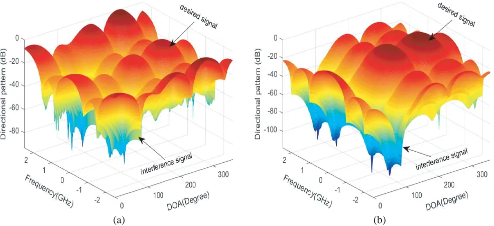
In this section, in order to evaluate the efficiency of the UCA-NW algorithm, several simulated examples are conducted to illustrate the results. Consider a UCA with M = 7 antenna elements, where each element is equally spaced with P = 5 taps. The signal to noise ratio (SNR) is set to −17 dB, and the jam to signal radio is set to 54 dB. Due to the long distance between satellites and receivers, the DOA of the desired satellite signal can be considered as constant. Assume that the DOA of the desired satellite signal is (280◦,30◦). In the simulation, suppose that there is one interference signal, that the initial DOA is (80◦,45◦), and that the DOA changes from (80◦,45◦) to (85◦,50◦). The weights are obtained by the snapshots at (80◦,45◦). The number of snapshots N is set to N = 1024.
(a) (b)
Figure 3. Beam pattern of MVDR algorithm and UCA-NW algorithm. (a) MVDR algorithm. (b) UCA-NW algorithm.
(a) (b)
Figure 4. Lateral view of MVDR algorithm and UCA-NW algorithm. (a) Lateral view of MVDR algorithm. (b) Lateral view of UCA-NW algorithm.
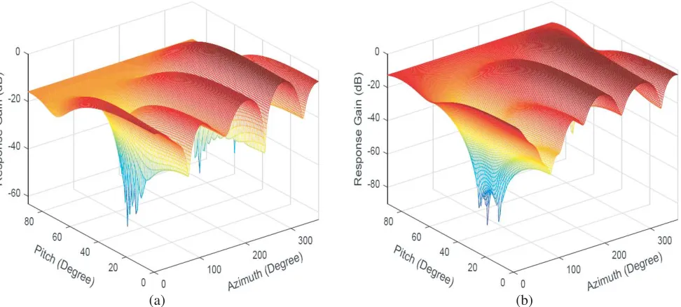
In order to analyse the null level clearly, the lateral views of MVDR algorithm and UCA-NW algorithm are given in Figure 4, respectively. From Figure 4, it is obvious that the azimuth angle of the interference signal is 80◦, and both of the algorithms can form a deep null at 80◦. Compared with conventional MVDR algorithm, the UCA-NW algorithm can broaden the null about 30◦ at the direction of interference signal. The UCA-NW algorithm can form a deeper null lever, and the null level of the UCA-NW algorithm is deeper than that of MVDR algorithm about 20 dB.
(a) (b)
Figure 5. Beam pattern of MVDR algorithm and UCA-NW algorithm. (a) MVDR algorithm. (b) UCA-NW algorithm.
0 50 100 150 200 250 300 350
Azimuth Angle (Degree)
0 10 20 30 40 50 60 70 80 90
Pitch Angle (Degree)
interference signal
0 50 100 150 200 250 300 350
Azimuth Angle (Degree)
0 10 20 30 40 50 60 70 80 90
Pitch Angle (Degree)
interference signal
(a) (b)
Figure 6. Contour of MVDR algorithm and UCA-NW algorithm. (a) Contour of MVDR algorithm. (b) Contour of UCA-NW algorithm.
than that of the MVDR algorithm distinctly.
In order to show the range of the formed null distinctly, the contours of MVDR algorithm and UCA-NW algorithm are plotted in Figure 6. In Figure 6, the azimuth angle range from 0◦ to 360◦ and the pitch angle range from 0◦ to 90◦. From Figure 6, it is clear that there is one interference signal located at (θ, φ) = (80◦,45◦). Moreover, the UCA-NW algorithm can explicitly broaden the width of the null about 30◦ from both azimuth angle and pitch angle, respectively.
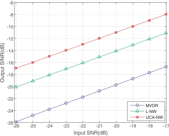
-26 -25 -24 -23 -22 -21 -20 -19 -18 -17
Input SNR(dB)
-26 -24 -22 -20 -18 -16 -14 -12 -10 -8 -6
Output SINR(dB)
MVDR L-NW UCA-NW
Figure 7. The output SINR versus input SNR.
about 3 dB and much higher than the MVDR algorithm about 10 dB. Because the null width of the UCA-NW algorithm is wider than that of MVDR algorithm, the performance of the UCA-NW algorithm is better than MVDR algorithm when the DOA of interference signals is changing.
5. CONCLUSIONS
This paper presents a novel null-widen algorithm based on the normal distribution model under uniform circular array to improve the performance of conventional space-time adaptive anti-jamming algorithms when the receiver is shaking. By using the extension matrix to modify the covariance matrix, the proposed UCA-NW algorithm can explicitly broaden the width of the null from azimuth angle and pitch angle, respectively, without the need to know the information of the interference signal. The results in simulation demonstrate that the proposed algorithm can not only suppress the interference signals effectively but also get a better null level.
ACKNOWLEDGMENT
This work was supported by the Natural Science Foundation of Hebei Province (Grant No. F2016501139), the Fundamental Research Funds for the Central Universities (Grant No. N172302002 and No. N162304002), and the National Natural Science Foundation of China (Grant No. 61501102).
REFERENCES
1. Kamath, V., Y. C. Lai, and L. Zhu, “ Empirical mode decomposition and blind source separation methods for antijamming with GPS signals,”Position, Location, And Navigation Symposium, 2006. 2. Lu, D., R. B. Wu, and Z. G. Sue, “A space-frequency anti-jamming algorithm for GPS,”Antennas
and Propagation Society International Symposium, 2007.
4. Ge, L., D. Lu, W. Wang, and L. Wang, “A high-dynamic null-widen GNSS anti-jamming algorithm based on reduced-dimension space-time adaptive processing,”China Satellite Navigation Conference, 2015.
5. Mailloux, R. J., “Covariance matrix augmentation to produce adaptive array pattern troughs,” Electronics Letters, Vol. 31, No. 10, 771–772, 1995.
6. Zatman, M., “Production of adaptive array troughs by dispersion synthesis,” Electronics Letters, Vol. 31, No. 25, 2141–2142, 1995.
7. Guerci, J. R., “Theory and application of covariance matrix tapers for robust adaptive beamforming,” IEEE Transactions on Signal Processing, Vol. 47, No. 4, 977–985, 1999.
8. Li W. X., Z. Yu, Y. B. Ye, and B. Yang, “Adaptive antenna null broadening beamforming against array calibration error based on adaptive variable diagonal loading,” International Journal of Antennas Propagation, Vol. 2017, No. 12, 1–9, 2017.
9. Jafargholi, A., M. Mousavi, and M. Emadi, “Wide-band VHF nulling by five elements spiral array antenna,” ITS Telecommunications Proceedings, 2006.
10. Yang, H. W. and J. G. Huang, “A broadband constant beam width adaptive beamforming method,” Computer Simulation, Vol. 10, No. 27, 339–342, 2010.
11. Liu, F. L., R. Y. Du, J. K. Wang, and B. Wang, “A robust adaptive control method for widening interference nulls,” IET International Radar Conference, 2009.
12. Li, W. X. and B. Yang, “An improved null broadening beamforming method based on covariance matrix reconstruction,”Applied Computational Electromagnetics Society Symposium, 2017. 13. Qian, J. H., Z. S. He, and Y. L. Zhang, “Null broadening adaptive beamforming based on
semidefinite programming,” Signal Processing, 2017.
14. Zhang, B. H., H. G. Ma, and X. L. Sun, “Robust anti-jamming method for high dynamic global positioning system receiver,”IET Signal Processing, Vol. 10, No. 4, 342–350, 2016.
15. Zetterberg, P. and B. Ottersten, “The spectrum efficiency of a basestation antenna array system for spatially selective transmission,” IEEE Transactions on Vehicular Technology, Vol. 44, No. 3, 651–660, 1995.
16. Riba, J., J. Goldberg, and G. Vazquez, “Robust beamforming for interference rejection in mobile communications,”IEEE Transactions on Signal Processing, Vol. 45, No. 1, 271–275, 1997.