The Axial Ratio of Planar Arrays with Random Element Errors

(1)

The Axial Ratio of Planar Arrays with Random Element Errors

Pedro M. Ruiz1, *, Randy L. Haupt2, Israel D. Hinostroza S´aenz1, and R´egis Guinvarc’h1

Abstract—Characterizing the random errors at the elements of a phased array antenna leads to equations that estimate the associated performance degradation. The increase in sidelobe level and decrease in gain due to random errors is well established. This paper derives an expression that predicts the axial ratio degradation due to random errors in the circularly polarized elements of an array. In the case of small errors in an array of crossed dipoles, we found a simple expression for the axial ratio of the array under random errors at broadside.

1. INTRODUCTION

Circularly polarized antenna arrays have many practical applications in communications and radar systems. Satellite communication arrays rely on circular polarization due to Faraday rotation of the signal as it passes through the ionosphere. Meteorological radar arrays must have very high isolation between vertical and horizontal polarization in order to distinguish between diﬀerent types of precipitation. Calibrating errors enhances the polarization isolation [1, 2].

Random array errors due to manufacturing tolerances, equipment aging, and temperature raise the sidelobe level and lower the gain of phased arrays. Traditionally, random errors in arrays have been analyzed to determine the impact on the sidelobe level. This paper looks at how random amplitude and phase errors change the axial ratio of a dual or circularly polarized planar array.

Ruze ﬁrst analyzed the impact of aperture errors on antenna patterns [3]. Random errors in an array are considered statistically independent from element to element. In this paper, position errors and random element failures are ignored, but amplitude and phase errors are not. These errors produce very broad array patterns that are superimposed on the no-error patterns resulting in “ﬁlled-in” nulls and the increased gain of low sidelobes [4, 5].

To the knowledge of the authors the analysis of the impact of array errors on the polarization purity of an array has not been done before (besides preliminary results in [6]). The goal of this paper is to model a circularly polarized planar array by an array of crossed dipoles with errors on the feeding currents in order to quantify the impact of array errors on the polarization.

In Section 2 we present the crossed dipoles array model for the planar array, and we deﬁne the errors in the feeding currents. In Section 3 we derive the approximate expression of the Axial Ratio (AR) as a result of the errors. In Section 4 we validate the resulting equation against the original model and observe the eﬀect of the errors with random trial simulations.

2. CROSSED DIPOLE ARRAY MODEL

In this section we present a model of a circularly polarized planar array of crossed dipoles with random amplitude and phase errors. In order to ﬁnd the AR of the crossed dipoles array, we calculate the

Received 24 June 2019, Accepted 9 August 2019, Scheduled 25 August 2019 * Corresponding author: Pedro Mendes Ruiz ([email protected]).

1 _{SONDRA Laboratory, CentraleSup´}_{elec, Ile-de-France 91190, France.} 2 _{Department of Electrical Engineering, Colorado School of}

(2)

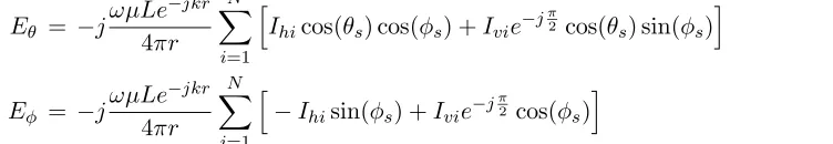
orthogonal linear electric ﬁelds of the array. We restrict the analysis to right handed polarized crossed dipoles in this paper, but the results apply to left handed polarized arrays as well because of the symmetry of the problem. If the two crossed dipoles have the same length, with one along the x-axis and the other along the y-axis [7]:

Eθ = −jωμLe

−jkr

4πr

Ihcos(θ) cos(φ) +Ivejπ2 cos(θ) sin(φ)

(1)

Eφ = −jωμLe

−jkr

4πr

−Ihsin(φ) +Ivejπ2 cos(φ)

(2)

whereω is the angular frequency;μis the space magnetic permeability; kis the wave number;r is the distance from the antenna to the observation point;I_h is the current on the horizontally oriented dipole; Iv is the current on the vertically oriented dipole;Lis the length of the dipoles;θis measured from the z-axis; andφ is measured from thex-axis.

If we neglect the mutual coupling between the different elements but feed each of the crossed dipoles with a different current, then the electric field of an array ofN crossed dipoles is given by

Eθ = −jωμLe

−jkr 4πr

N

i=1

e−jδ_posi_I

hicos(θ) cos(φ) +Iviejπ2 cos(θ) sin(φ) (3)

Eφ = −jωμLe

−jkr

4πr N

i=1

e−jδposi₋_I_hi_sin(_φ_{) +}_I_vi_ejπ2 cos(φ) (4)

δposi =

2π λ

sin(θ) cos(φ)−sin(θ_s) cos(φ_s)x_i+sin(θ) sin(φ)−sin(θ_s) sin(φ_s)y_i

(5)

where [x_i, y_i] is the position of theith crossed dipoles element. Errors are assumed to be amplitude and phase deviations from the desired current.

Ihi = I(1 +δI_hi)e−jφhi ₍₆₎

Ivi = I(1 +δI_vi)e−jφvi ₍₇₎

whereδI_hi,δI_vi,δφ_hi, andδφ_vi are, respectively: the horizontal dipole normalized amplitude error, the vertical dipole normalized amplitude error, the horizontal dipole phase error, and the vertical dipole phase error for the i-th crossed dipoles element.

3. AXIAL RATIO FORMULA FOR AN ARRAY WITH RANDOM ELEMENT ERRORS

This section presents the derivation of the AR expression for the crossed dipoles array with errors. By means of a simple normalization, observing the broadside radiation without steering ([θ, φ] = [θ_s, φ_s] = [0,0]) and using Equations (6) and (7), (3) and (4) reduces to the following equations:

Eθ = N

i=1

(1 +δI_hi)e−jδφhi ₍₈₎

Eφ = ejπ2

N

i=1

(1 +δI_vi)e−jδφvi ₍₉₎

At this point we consider the errors to be small and make the Taylor expansionex = 1 +x+O(x2), as well as neglect the terms δI_hiδφ_hi and δI_viδφ_vi. Next, decomposing the ﬁelds into right and left handed polarization components using (A1) and (A2) (see Appendix), results in:

Erhp = √1 2

N

i=1

(2 +δI_hi+δI_vi−jδφ_hi−jδφ_vi) (10)

Elhp = √1 2

N

i=1

(3)

These equations simplify to:

Erhp = √1

2(2N +δI+−jδφ+) (12)

Elhp = √1

2(δI−−jδφ−) (13)

where:

δI− = N

i=1

(δI_hi−δI_vi) (14)

δφ− = N

i=1

(δφhi−δφvi) (15)

δI+ = N

i=1

(δI_hi+δI_vi) (16)

δφ+ = N

i=1

(δφhi+δφ_vi) (17)

Finally, by using Equations (A5) (see Appendix A), (12) and (13) we get:

AR= 20

Nln (10)

δI2

−+δφ2−

1 + δI+ 2N

2 +

δφ+ 2N

2 (18)

Assuming that the terms δI₂_N+ and δφ₂_N+ are small enough to neglect, then we get:

AR= 20

Nln (10)

δI2

−+δφ2− (19)

The AR of the array depends on the diﬀerence between the amplitudes and phases of the horizontal and vertical dipole currents. Random errors at the elements average, so Equation (19) is proportional to _N1.

4. RESULTS

In this section, results at boresight and scan angle are presented.

4.1. Axial Ratio at Boresight

In order to validate Equation (19), we calculated the AR of one crossed dipole element for 106 random amplitude and phase errors. The errors are zero-mean, normally distributed with standard deviations of σ_φ_h = σ_φ_v = 0.2 (11.46◦) and σ_I_h = σ_I_v = 0.1 (10%). We calculated the AR using Equation (19), then created the histograms in Figure 1 and calculated the ﬁgures of merit shown in Equations (20), (21), (22), and (23). We used the formula (2n)1/3, withnthe sample size (106), to calculate the number of bins in the histograms [8]. To calculate the bin width for the histogram we considered the range of values to be contained between 0 dB and 10 dB, which gives a bin width of 0.08 dB.

|AR−ARapprox|99% = 0.68 dB (20)

|AR−ARapprox|95% = 0.32 dB (21)

1 N

N

i=1

(4)

0 2 4 6 8 10 0

1 2

·104

0 2 4 6 8 10

0 1 2

·104

AR (dB)

Number of Realizations in the bin Number of Realizations in the bin

AR (dB)

(a) (b)

Figure 1. Histogram of the random trial simulations of the AR calculations for a single crossed dipole element at broadside. (a) With approximations in (19), (b) without approximations. In dashed red we have the AR without errors (0 dB). The bins in the histogram have a 0.08 dB width.

1 N

N

i=1

ARi−ARapproxi

ARi

= 3% (23)

This example demonstrates that the approximate equations derived in the last section accurately predict the change in AR due to small random errors at the elements.

In the case where all the errors are independent identically distributed Gaussian with zero mean, Equation (19) follows a Rayleigh distribution. By looking at the histograms we can see that even when the errors have diﬀerent standard deviations they present a Rayleigh-like behaviour.

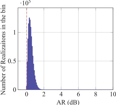
In order to observe the eﬀect of having more than one element, we made the same test for a small uniform 5×5 planar array with a spacing ofλ/2 (Figure 2). We can observe that, as it can be predicted from Equation (19), the more elements we add to the array, the smaller the variance on the results, which get closer to the ideal case without errors.

0 2 4 6 8 10

0 0.5 1

·105

Number of Realizaitons in the bin

AR (dB)

(5)

4.2. Axial Ratio at Scan Angle

Scanning the main beam away from broadside makes the calculations for the AR much more complicated. However, it is simple to make a random trial simulation of the AR at the steering direction. Using Equations (3), (4), and (5) and making [θ, φ] = [θ_s, φ_s] we get:

Eθ = −jωμLe

−jkr 4πr

N

i=1

Ihicos(θs) cos(φs) +Ivie−jπ2 cos(θ_s) sin(φ_s)

(24)

Eφ = −jωμLe

−jkr

4πr N

i=1

−Ihisin(φs) +I_vie−jπ2 cos(φ_s)

(25)

Note that in the steering direction, the radiated ﬁelds are no longer a function of the element positions, since the electronic phase applied to each element compensates the phase due to the position of the element in the steering direction.

For this simulation, we will consider ﬁrst a single element looking at the steering direction (Figure 3), then a small uniform 5×5 planar array with a spacing of λ/2 (Figure 4). The errors are independent Gaussian distributed, with the amplitude errors having a standard deviation σ_I_h = σ_I_v = 0.1 (10%) and the phase errors σ_φ_h = σ_φ_v = 0.2 (11.46◦). For the simulation we will consider a steering of [θ_s, φ_s] = [30◦,0◦], which give an AR of 1.25 dB for an array without errors.

0 2 4 6 8 10

0 1 2

·104

AR (dB)

Number of Realizations in the bin

Figure 3. Histogram of the random trial simulations of the AR calculations without approximations for a single crossed dipoles element at 30◦. In dashed red we have the AR without errors (1.25 dB). The bins in the histogram have a 0.08 dB width.

0 2 4 6 8 10

0 0.5 1

·105

AR (dB)

Number of Realizaitons in the bin

Figure 4. Histogram of the random trial simulations of the AR calculations without approximations for 25 crossed dipoles elements scanned to 30◦. In dashed red we have the AR without errors (1.25 dB). The bins in the histogram have a 0.08 dB width

Figure 3 shows that the AR of the isolated element at the steering direction degrades when errors are considered. Comparing the broadside case in (Figure 1) with the scanned case in Figure 3, we observe that the AR degrades oﬀ-broadside.

In Figure 4, we observe that the AR from the random trial simulations is nearly the same as the estimate calculated using errorless feeding currents. The random trial simulations get closer to the errorless case as the number of elements in the array increases.

5. CONCLUSION

(6)

depends on the diﬀerence between the amplitudes and phases of the horizontal and vertical dipole currents. Random trial simulations validate the approximate formulas for broadside arrays and are used to explore scanned arrays.

We observe that considering the feeding errors to be independent identically distributed Gaussian variables, the expression in Equation (19) leads to a Rayleigh probability density function. Equation (19) also predicts that, as the number of elements (N) in the array gets larger, random errors have less impact on the AR of the array due to averaging, which is veriﬁed in Figure 2 and Figure 4.

APPENDIX A. AXIAL RATIO EXPRESSION

Having the linear polarized ﬁelds (E_θ andE_φ), we can calculate the right handed and left hand polarized electric ﬁelds (E_rhp and E_lhp) using the following equations:

Erhp = √1

2(Eθ−jEφ) (A1)

Elhp = √1

2(Eθ+jEφ) (A2)

We can then calculate the cross polarization ratio and ﬁnd the AR with the following equations:

xpolr2 ₌ |Erhp|2

|Elhp|2 (A3)

AR = 20 log₁₀

xpolr+ 1 xpolr−1

, xpolr >1 (A4)

which means that|E_rhp|>|E_lhp|(a reasonable assumption for a right handed polarized antenna). By taking the Laurent series of ln(x_x+1₋₁), asx→ ∞, we get 2_x+O(_x1₃), which gives an approximation for the AR expression, that becomes the following by combining Equations (A3) and (A4):

AR= 40

ln (10)

|Elhp|2

|Erhp|2 (A5)

REFERENCES

1. Fulton, C. and W. J. Chappell, “Calibration of a digital phased array for polarimetric radar,”2010

IEEE MTT-S International Microwave Symposium, 161–164, Anaheim, CA, 2010.

2. Fulton, C., M. Yeary, D. Thompson, J. Lake, and A. Mitchell, “Digital phased arrays: Challenges and opportunities,”Proceedings of the IEEE, Vol. 104, No. 3, 487–503, March 2016.

3. Ruze, J., “Antenna tolerance theory — A review,” Proceedings of the IEEE, Vol. 54, 633–640, April 1966.

4. Brookner, E., “Antenna array fundamentals — Part 2,” Practical Phased Array Antenna Systems, E. Brookner, Artech House, Norwood, MA, 1991.

5. Haupt, R. L., Antenna Arrays: A Computational Approach, Wiley, Hoboken, NJ, 2010.

6. Ruiz, P. M., I. Hinostroza, R. Guinvarc’h, and R. L. Haupt, “Antenna pattern eﬀects in a low sidelobe circularly polarized array due to element errors,” Proceedings of the International

Conference on Electromagnetics in Advanced Applications (ICEAA — IEEE APWC), Cartagena,

Colombia, September 10–14, 2018.

7. Haupt, R. L., “Adaptative crossed dipole antennas using a genetic algorithm,” IEEE Transactions

on Antennas and Propagation, Vol. 52, No. 8, 1976–1982, August 2004.

8. Terrell, G. and D. Scott, “Oversmoothed nonparametric density estimates,” Journal of the