Shape Reconstruction of Unknown Targets Using Multifrequency
Linear Sampling Method
Mallikarjun Erramshetty*
Abstract—This paper aims to estimate the shape of microwave scattering objects using linear sampling method (LSM) with multifrequency data. LSM is a simple, reliable linear inverse algorithm and uses multiview multistatic single frequency scattered field data measured around target objects. Despite its simplicity and computational effectiveness, the output LSM results depend on the frequency of operation. To improve the LSM performance, the present work proposes a new formulation that incorporates frequency information in the LSM equation. As a result, LSM finds the target’s shape by a simple solution to a linear inverse problem via multifrequency data. The output results are tested with various types of numerical examples of synthetic data as well as experimental data provided by the Institute of Fresnel.
1. INTRODUCTION
Geometric features estimation of unknown objects has many applications in the field of military, civil, industrial, and so on [1]. Linear sampling method (LSM) is a simple, reliable and effective tool to estimate the shapes and locations of the dielectric and/or the metallic objects through multi-view-multistatic measured scattered fields [2]. In addition, it has very low computational time [3]. Despite having many advantages, the method is frequency dependent [4]. At low frequencies, it is unable to estimate target’s shape accurately. At higher frequencies, LSM fails to detect the target points at certain frequencies due to the occurrence of eigenvalues [5]. To overcome single frequency drawbacks, multifrequency approaches are adopted [5–8]. Wherein, the LSM indicator is modified to exploit the reconstructions computed at each considered frequency. However, this procedure requires regularized LSM solution for each frequency and a suitable design of multifrequency indicator function. In this work, we incorporate frequency information in the governing equation. As a result, the problem can be cast as a single linear inversion so that it does not require a solution of LSM equation for each frequency. In addition, one-time estimation of regularization parameter is required only. The results are tested for the cases of dielectric objects, conducting objects, and mixed boundary objects using synthetic data as well as experimental data. In addition, the computed results are compared with other LSM multifrequency methods. The rest of the paper discusses the multifrequency linear sampling method, numerical results, and conclusion.
2. MULTIFREQUENCY LINEAR SAMPLING METHOD
For simplicity, we consider a two-dimensional scalar problem. Target objects are illuminated by a plane wave of radial frequency ω from a direction ϕi. Polarization currents are induced in the objects that results in scattering. These scattered fields are measured at far-field distancer. According to LSM, the
Received 1 November 2018, Accepted 18 December 2018, Scheduled 13 January 2019
targets’ support is estimated through the solution of far-field equation given by [2],
A[ξ] =
2π
0
Escat(r, ϕi, ω)ξ(zt, ϕi, ω)dϕi=G(r, zt, ω) (1)
Escat is the measured scattered field; G is a point source; zt = (x, y) is a sampling point that spans the considered investigation area (Ω);ξ is an unknown weighted complex function; andA is a compact far-field operator [2]. In a standard LSM implementation, Eq. (1) is to be solved for a given single frequency data. The solution in the energy formξ2 is bounded ifzt belongs to the scatterer support and unbounded elsewhere [2]. Here, ·2 is the standard L2-norm. Hence, the support of the scatterer is found by plotting regularized ξ2 at each sampling point over investigation domain. Let us consider the case of multifrequency. The far-field Eq. (1) is to be discretized with respect to ω along withr and ϕi. LetM be the number of measurements for each incident field. N is the number of incident fields, and F is the number of considered frequencies. Then, the discretized version of Eq. (1) is represented synthetically as
Aξ=b (2)
where A,ξ, and bare defined by
A=
⎡ ⎢ ⎣
A1 0 0 . . . 0
0 A2 0 . . . 0
. . . . . . . . . . 0 0 0 . . . AF
⎤ ⎥ ⎦
(M×F)×(N×F)
, ξ = ⎡ ⎢ ⎣ ξ1 ξ2 . . . ξF ⎤ ⎥ ⎦
(N×F)×1
, b=
⎡ ⎢ ⎣ b1 b2 . . . bF ⎤ ⎥ ⎦
(M×F)×1
.
Here [A1]M×N, [A2]M×N, . . ., [AF]M×N represent scattered field data measured for each frequency.
Vectors [b1]M×1, [b2]M×1, . . ., [bF]M×1 represent the far-field pattern radiated by the point source
located atzt. [ξ1]N×1, [ξ2]N×1, . . ., [ξF]N×1 are the vectors of unknown and independent. In order to
find target’s shape, Eq. (2) is to be solved. This is an ill-posed equation and requires regularization for a stable solution. Tickhonov regularization is a suitable option to pursue this task. While referring the reader to [2, 9] for mathematical details, the final form of regularized solution based on the singular value decomposition (SVD) technique [1] can be written as
ξ(zt)2= T
n=1
λn λ2
n+α
2
|b·μn|2 (3)
whereλnandμnare singular-values and left singular vector ofA, respectively. T is the total number of non-zero singular values,T = min(M ×F, N×F), andα is a regularization parameter. Therefore, the support of the scatterer is found by plottingξ2 =ξ1+ξ2+. . .+ξF2 for each sampling point over
the investigating domain. In general, LSM requires regularization parameter for each sampling point and it is cumbersome. In [10], it is shown that one regularization parameter is sufficient to get good results. In this work, parameter α is estimated using physics-based criteria as reported in [11], which does not require knowledge about noise level present in the measured data. It is worth to mention that the proposed form of solution is not completely different from other multifrequency approaches [5–8]. The analogy between the present method to the earlier approaches is detailed in Appendix A.
3. NUMERICAL RESULTS AND DISCUSSION
3.1. Dielectrics
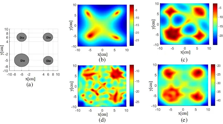
In this example, we consider three circular dielectric cylinders of radius 2 cm each and a circular dielectric cylinder of radius 3 cm. The relative permittivity of these objects hasr = 3 and are located as shown in Fig. 1(a). The computed LSM results at 1 GHz, 3 GHz, 6 GHz, and multifrequency are shown in Fig. 1(b) through Fig. 1(e). For better visibility, the output values (intensity) are plotted by−10 log(ξ2) dB. It can be observed that only a small portion of each object is detected properly at 1 GHz. When the frequency is increased, the images of dielectric objects improve as seen for 3 GHz. However, at 6 GHz, the central portion of the larger cylinder is undetected. This anomaly behavior can be reasoned based on the occurrence of eigenvalues. According to [5], the chance of occurrence of eigenvalues increases with increase in frequency, as a result, LSM fails to detect target sampling points. Fig. 1(e) shows the obtained results using multifrequency approach. Good estimates are observed with the proposed multifrequency approach, and it can be seen that these results are superior to the case of single frequency. It can be noted that the range of intensity values vary around−5 dB to−25 dB for a single frequency case whereas for multifrequency, the range is around−20 dB to −40 dB. The reason is as follows. At multifrequency, the output values,ξ2, are much greater than a single frequency values (ξ12,ξ22, . . . , ξF2). As
a result −10 log(ξ2) <(−10 log(ξ12), −10 log(ξ22), . . . , −10 log(ξF2)). It is worth to mention
that this multifrequency procedure cannot eliminate the drawbacks of each frequency completely but certainly will produce a better estimation than individual frequencies.
(b)
(a)
(d)
(c)
(e)
Figure 1. (a) Reference profile. (b) 1 GHz,α= 0.0027. (c) 3 GHz,α= 0.0118. (d) 6 GHz,α= 0.0091. (e) Multifrequency,α= 0.0016. The intensity values are in dB.
3.2. Conductors
(b)
(a)
(d)
(c)
(e)
Figure 2. (a) Reference profile. (b) 1 GHz,α= 0.0375. (c) 3 GHz, α= 0.0173. (d) 6 GHz, α= 0.008. (e) Multifrequency,α= 0.04. The intensity values are in dB.
3.3. Mixed Boundary Objects
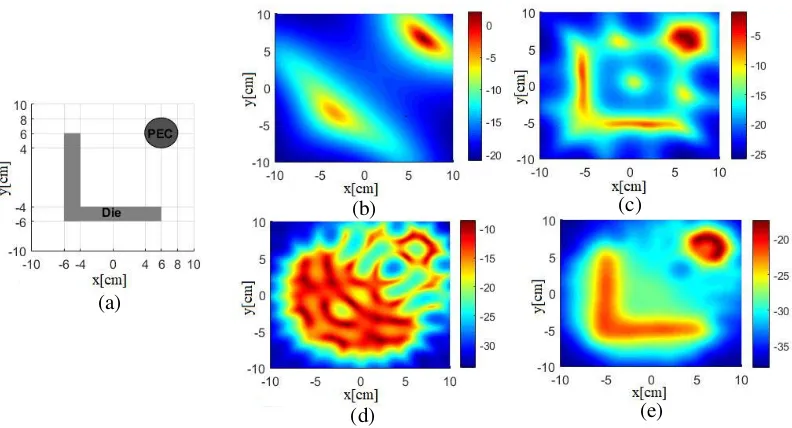
This example consists of an L-shape dielectric object in presence of a circular PEC cylinder of radius 2 cm. Each arm of the L-shape has length and breadth of 12 and 2 cm, respectively, and r = 2. The results of LSM at 1 GHz, 3 GHz, 6 GHz, and multifrequency are shown in Fig. 3(b) to Fig. 3(e). The dielectric object is not recognizable at lower frequencies whereas, with the increase in frequency, the estimation of dielectric shape improves. At higher frequency, 6 GHz, both dielectric and PEC objects get affected by the occurrence of eigenvalues. In the case of multifrequency, the drawbacks of low and high frequencies are overcome, and the estimated results are more accurate.
(b)
(a)
(d)
(c)
(e)
3.4. Results on Experimental Data
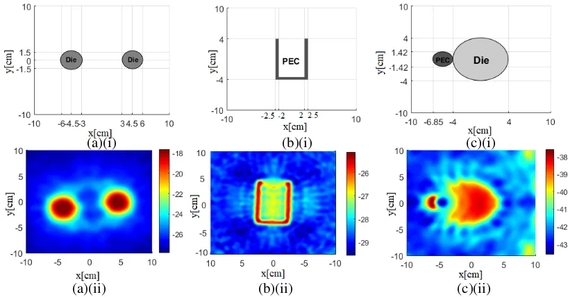
In this example, we consider experimental datasets provided by the Institute of Fresnel, France. While addressing the reader to [12, 13] for detailed description, a few details about the measurement procedure are as follows. In their measurement setup, only one transmitting horn antenna (TX) and receiving horn antenna (RX) pair had been used. For each transmitted field, the receiver will move around the investigation domain to measure the scattered fields from sample objects. The procedure is repeated for several frequencies. In this work, three types of reference object profiles are selected for the study: first, two dielectric objects of radius 1.5 cm having relative permittivity r = 3; second, a U-shaped metallic object having an arm length of 8 cm and a width of 0.5 cm; third, PEC cylinder of diameter 2.85 cm along with a foam cylinder of diameter 8 cm and r = 1.45. These objects are shown in Fig. 4. The considered scattered fields from the available measurements are as follows. First and second objects were sequentially illuminated at 0◦, 10◦,. . ., 350◦ with 10◦incremental angular step. In each illumination, the scattered fields from 60◦ to 300◦ with 5◦ angular step with reference to the transmitter are considered. The fields at non-available positions are assumed to be zero. Third object was sequentially illuminated at 0◦, 20◦,. . ., 340◦ with 20◦incremental angular step. In each illumination, the scattered fields from 60◦ to 300◦ with 5◦ angular step with reference to the transmitter are chosen. The considered frequencies from the available measurements are: for dielectrics, 1 GHz to 18 GHz with the span of 1 GHz; for the metallic object, 1 GHz to 18 GHz with the span of 2 GHz; for mixed boundary objects, 2 GHz to 12 GHz with the span of 1 GHz. Similar to the synthetic examples, targets’ shape is not retrieved properly at low-frequencies, and at high frequencies, the shapes get affected by the eigenvalues. It can be seen that multifrequency results (as shown in Figs. 4a(ii), b(ii) and c(ii)) are in close match with reference profile, and these are better than the cases of single frequency. Due to space constraints, the single frequency images are not shown here.
(b)(i)
(a)(i) (c)(i)
(b)(ii)
(a)(ii) (c)(ii)
Figure 4. Experimental results. a(i) Reference two-dielectrics profile. a(ii) Multifrequncy result, α = 0.0786. b(i) Reference U-shaped conductor profile. b(ii) Multifrequency result, α = 0.0370. c(i) Reference mixed-boundary objects. c(ii) multifrequency result,α= 0.0013. The intensity values are in dB.
3.5. Comparison of Results with Multifrequency Indicator Function
given by
G(zt) =−10 log
⎛ ⎜ ⎝1
F F
i=1
ξ(zt, i)2 max
r∈Ω ξ(zt, i) 2
⎞ ⎟
⎠ (4)
The above equation shows that the individual plots are normalized. The comparison results for the considered synthetic examples are shown in Fig. 5. Here, frequencies from 1 GHz to 6 GHz with the span of 0.5 GHz are considered. It can be observed that better reconstructions are obtained with the proposed approach. In specific, the contrast between the object and the background is more with the proposed approach. Notably, the new results are definitely better than a single-frequency case.
(b)(i)
(a)(i) (c)(i)
(b)(ii)
(a)(ii) (c)(ii)
Figure 5. Comparison of multifrequency LSM Results: (a) with the multifrequency indicator function reported in [8]; (b) With our multifrequency LSM: (i) Example I, (ii) Example II, and (iii) Example III. The intensity values are in dB.
4. CONCLUSION
In this paper, the shape reconstruction of dielectric and/or conducting objects is estimated using linear sampling method (LSM) with multifrequency data. The LSM equation is made as a function of frequency so that the target’s support estimation has been done through the solution to a regularized linear inverse problem. As a result, the proposed approach requires one-time estimation of the regularization parameter only. It has been observed that the estimated results are better than the case of single frequency. This multifrequency approach cannot eliminate the drawbacks of each frequency completely but certainly will produce a better estimation than individual frequencies. The numerical results have been tested with the synthetic data as well as the experimental data for various types of objects.
APPENDIX A.
The general form of multifrequency indicator function is [8],
ξ2
Here, a1, a2, . . . , aF are the factors of normalization. The proposed form of solution can be
represented as follows.
ξ2 =ξ
1+ξ2+. . .+ξF2 (A2)
=ξ12+ξ22+. . .+ξF2+ξ1ξ∗2+ξ2ξ1∗+. . .+ξ1ξ∗F +ξFξ1∗+. . .+ξFξF∗−1+ξF−1ξF∗ (A3)
=ξ12+ξ22+. . .+ξF2±real number (A4)
Here,∗indicates complex conjugate. From equations (A1) and (A4), it can be noted that each term in the former equation is weighted with normalization factor while the later one is added/subtracted with some real number. With this modification, the output results in the proposed case are found to be better. However, it requires more mathematical analysis to support these findings, and these are treated as future works.
REFERENCES
1. Pastorino, M., Microwave Imaging, 82–91, Hoboken, NJ, USA, Wiley, 2010.
2. Colton, D., H. Haddar, and M. Piana, “The linear sampling method in inverse electromagnetic scattering theory,”Inv. Prob., Vol. 19, 105–137, 2003.
3. Catapano, I., F. Soldovieri, and L. Crocco, “On the feasibility of the linear sampling method for 3D GPR surveys,”Progress In Electromagnetics Research, Vol. 118, 185–203, 2011.
4. Shelton, N. and K. F. Warnick, “Behavior of the regularized sampling inverse scattering method at internal resonance frequencies,” Progress In Electromagnetics Research, Vol. 38, 29–45, 2002. 5. Mallikarjun, E. and A. Bhattacharya, “Shape reconstruction of mixed boundary objects by linear
sampling method,”IEEE Trans. Antennas Propagat., Vol. 63, No. 7, 3077–3086, 2015.
6. Sun, J., “An eigenvalue method using multiple frequency data for inverse scattering problems,” Inv. Prob., Vol. 28, No. 8, 025012, 2012.
7. Guzina, B., F. Cakoni, and C. Bellis, “On the multi-frequency obstacle reconstruction via the linear sampling method,”Inv. Prob., Vol. 26, No. 12, 125005, 2010.
8. Catapano, I., L. Crocco, and T. Isernia, “Improved sampling methods for shape reconstruction of 3-D buried targets,” IEEE Trans. Geosci. Remote Sens., Vol. 46, No. 10, 3265–3273, 2008.
9. Colton, D. and H. Haddar, “An application of the reciprocity gap functional to inverse scattering theory,” Inv. Probl., Vol. 21, No. 1, 383–398, 2005.
10. Bozza, G., M. Brignone, and M. Pastorino, “Application of the no-sampling linear sampling method to breast cancer detection,”IEEE Trans. Antennas Propag., Vol. 57, No. 10, 2525–2534, Oct. 2010. 11. Catapano, I. and L. Crocco, “An imaging method for concealed targets,” IEEE Trans. Geosci.
Remote Sens., Vol. 47, No. 5, 1301–1309, May 2009.
12. Belkebir, K. and M. Saillard, “Special section: Testing inversion algorithms against experimental data,” Inv. Prob., Vol. 17, 1565–1571, 2001.
![Figure 5. Comparison of multifrequency LSM Results: (a) with the multifrequency indicator functionreported in [8]; (b) With our multifrequency LSM: (i) Example I, (ii) Example II, and (iii) ExampleIII](https://thumb-us.123doks.com/thumbv2/123dok_us/7735208.1266671/6.612.108.513.226.432/comparison-multifrequency-results-multifrequency-indicator-functionreported-multifrequency-exampleiii.webp)
