PHSS Iterative Method for Solving Generalized Lyapunov Equations

(1)

PHSS Iterative Method for Solving Generalized

Lyapunov Equations

Shi-Yu Li,Hai-Long Shen* _{and Xin-Hui Shao}

Department of Mathematics , College of Sciences, Northeastern University, Shenyang, China.

Abstract: Based on previous research results, we propose a new preprocessing HSS iteration method (PHSS) for the generalized Lyapunov equation. At the same time, the corresponding inexact PHSS algorithm (IPHSS) is given from the angle of application. All the new methods presented in this paper have given the corresponding convergence proof. The numerical experiments are carried out to compare the new method with the existing methods, and the improvement effect is obvious. The feasibility and effectiveness of the propos method are proved from two aspects of theory and calculation.

Keywords Lyapunov equation; HSS iterative method; PHSS iterative method

1. Introduction

We consider the system of large sparse linear equations

,

Ax b= (1) where _{A C}_∈ n n× _{is non-Hermite positive definite matrix and ,}_{x b C}_∈ n n× _._{The actual}

background of such problems can be found in [1, 2, 3, 4, 5, 6, 7] and its references. For (1), Bai, Golub and Ng put forward the HSS[8]_{iteration method in 2003.}

Any matrix can be decomposed into the sum of symmetric matrices and skew symmetric matrices so that we can get the formula:

( ) ( ) ( ( )) ( ( )) ( ( )) ( ( )), A H A= +S A = αI H A+ − αI S A− = αI S A+ − αI H A−

where α is normal number, ( ) 1( )

2

H A ₌ A A₊ ∗ _, _{( )} 1₍ ₎

2

S A ₌ A A₋ ∗ _{, and}

( ), ( ) n n

H A S A _∈C × _{, As a result, the HSS iterative format proposed by Bai and others}

is:

Let (0) n

x ∈C be an initial guess. For k=0,1, 2,..., until the sequence of iterates _{_x( )k_}_{converges, compute the next iterate} _x(k+1)_{through the following}

procedure:

---

(2)

* Corresponding author. E-mail address: [email protected].

** Project supported by the National Natural Science Foundation of China (No. 11371081) and

the Natural Science Foundation of Liaoning Province (No. 20170540323). 1

( ) _{( )}

2

1 ( )

( 1) 2

( ( )) ( ( )) ,

k _k

k k

I H A x I S A x b

I S A x I H A x b

α α

+

+ +



+ = − +

 

 ₊ ₌ ₋ ₊



where α is normal number. Bai and others proved its unconditional convergence to the unique solution of (1) in [8].

In order to speed up the HSS iteration method, Bai and others put forward the

PHSS iteration method [9-11]. Decompose coefficient matrix A into the sum of

symmetric matrices and skew symmetric matrices and we can get the formula:

( ( ) ( )) ( ( ) ( )) ( ( ) ( )) ( ( ) ( )), A= αP A +H A − αP A −S A = αP A +S A − αP A −H A (2) where _{P A}( )_∈_Cn n× _{is Hermite positive definite matrix. Therefore, we can get the}

HSS iterative format:

1

( ) _{( )}

2

1 ( )

( 1) 2

( ( ) ( )) ( ( ) ( )) ,

k _k

k k

P A H A x P A S A x b

P A S A x P A H A x b

α α

+

+ +



+ = − +

 

 ₊ ₌ ₋ ₊



where α is normal number. Bai and others proved its unconditional convergence to the unique solution of (1) in [10].

2. The PHSS iterative method for the generalized Lyapunov equation

Many methods to solve the standard Lyapunov equation have been put forward

in [12-19].In the literature [12], Xu Qingqing and others put forward the HSS iterative

solution of the generalized Lyapunov equation. Inspired by this, this paper proposes

the PHSS iterative solution of the generalized Lyapunov equation.

Consider the generalized Lyapunov equation as follows:

1

0, m

j j j

AX XAΤ N XNΤ C

=

+ +



+ = (3)

where , , n n

j

A N C R_∈ × _{, A is an asymmetric positive definite matrix, C is a symmetric}

matrix and ₂

2 ( 1, 2..., )

j

(3)

standard Lyapunov equation.

Then we apply the PHSS iterative method to solve the generalized Lyapunov

equation (3):

Let's suppose that α is a normal number, then the decomposition of A is similar to (2):

( ( ) ( )) ( ( ) ( )) ( ( ) ( )) ( ( ) ( )),

A P A H A P A S A P A S A P A H A

α α α α

Τ

= + − − = + − −

= + − + = − − −

Then the iterative format can be obtained:

1 1 2 2 1 1 1 1 1 2 2 ( ( ) ( )) ( ( ) ( )) ( ( ) ( )) ( ( ) ( )) , ( ( ) ( )) ( ( ) ( )) ( ( ) ( )) ( ( k k m

k k j k j

j

k k

P A H A X X P A H A

P A S A X X P A S A N X N C P A S A X X P A S A

P A H A X X P A

α α α α α α α α + + Τ = + + + + + + + = − + + − − + + − = − +



1

) ( )) m _j _k _j ,

j

H A N X N Τ C

=          ₋ ₋ ₋ 



(4)

According to the nature of Kronecker product, we can get

1 2 1 1 ( ( ) ( ( ) ( )) ( ( ) ( )) ( )) ( ( ) ( ( ) ( )) ( ( ) ( )) ( )) ( ) , ( ( ) ( ( ) ( )) ( ( ) ( )) ( )) ( ( ) ( ( ) ( )) ( ( ) ( )) k m

k j j k

j k

I A P A H A P A H A I A x

I A P A S A P A S A I A x N N x c

I A P A S A P A S A I A x

I A P A H A P A H A

α α α α α α α α + = + ⊗ + + + ⊗ = ⊗ − + − ⊗ − ⊗ − ⊗ + + + ⊗ = ⊗ − + −



1 1 2

( )) m ( _j _j) _k ,

k _j

I A x N N x c

+ ₌          _⊗ ₋ _⊗ ₋ 



where x_k =vec X( _k),c vec C= ( ),then, according to the nature of Kronecker product, we can get

1 1 2 1 1 1 2 ( ) ( ) ( ) , ( ) ( ) ( ) , m

k j j k

k _j

m

k _k j j k

j

P H x P S x N N x c

P S x P H x N N x c

α α α α + ₌ + ₊ =  + = − − ⊗ −     ₊ ₌ ₋ ₋ _⊗ ₋ 



(5)

where

( ) ( ) ( ) ( ),

( ) ( ) ( ) ( ).

P I A P A P A I A H I A H A H A I A

S I A S A S A I A

= ⊗ + ⊗   = ⊗ + ⊗   ₌ _⊗ ₊ _⊗ 

(4)

iterative scheme (5) and their convergence factors are the same.

Theorem 1. Let's suppose that _{A R}_∈ n n× _{is an asymmetric positive definite matrix,}

1 2

1 ₂

m

j j

j

K P− N N

=



⊗ and the maximum and minimum eigenvalues of matrix

1

P H− _are

max

λ and _λ_min, respectively. Then the convergence factor of the PHSS

iterative method (4) is the spectral radius of matrix

1 1 1 1

1

( ) ( )( ) ( ) 2 ( ) ( ) m ( _j _j).

j

G _αP S − _αP H _αP H − _αP S _{α α}P P S − _αP H − N N

=

= + − + − − + +



⊗

Its upper bound is

1

0

( )

min

2

( ) max .

i

i P H

i

K

λ λ

α λ σ α

α λ α λ

−

∈

−

= +

+ +

When _λ_min >K and _α= _λ_min⋅_λ_max , _{σ α}₀( ) reaches the minimum. It means that

min max min 0

min max min

2

( ) λ λ λ K 1,

σ α

λ λ λ

⋅ − +

= <

⋅ +



Therefore,the PHSS iterative method for solving the generalized Lyapunov equation

is convergent.

Proof. The first form of the iteration format (5) is brought into the second form, and its iteration matrix is obtained:

1 1

1

( ) ( )( ) ( )

2 ( ) ( ) ( ),

m

j j

j

G P S P H P H P S

P P S P H N N

α α α α

α α α

− −

=

= + − + −

− + +



⊗

Then the convergence factor of the iterative scheme (5) is ρ( )G , which is the same as the convergence factor of the iterative scheme (4).

Because _{P R}_∈ n n× _{is a symmetric positive definite matrix, we can suppose that}

1 1 1 1

2 2_, 2 2_. H =P HP− − S=P SP− −

(5)

1 1

1 1 1

1

( ) ( )

( )( ) ( )( )

2 ( ) ( ) ( ) m ( _j _j)( )

j

G P S G P S

P H P H P S P S

P S P P S P H N N P S

α α α α α α α α α α α − − − − − − = = + − = − + − + − + + +



⊗ +

and G1 is similar to 1 1 2 2

2 1

1 1 1 1 1 1 1 1 1 1

1 1

2 2 2 2 2 2 2 2 2 2

1 1 1 1 1 1 1

1 1

2 2 2 2 2 2 2

1

1 1 1

1

2 2 2

1 1

( ) ( ) ( ) ( )

2 ( ) ( ) ( ) ( )

( )

( )( ) ( )( )

m

j j

j G P G P

P P I H P P I H P P I S P P I S P P

P P I S P PP I S P P I H P N N

P P S P P

I H I H I S I S

α α α α α α α α α α α α α − − − ₋ − − ₋ − − − ₋ − − ₋ − = − ₋ − − − = = − + − + − + + + ⊗ ⋅ + = − + − +



           1 1

1 1 1 2 2 1

1

2 ( ) ( ) ( ) m ( _j _j) ( ) ,

j

I S P I S P I H P N N P I S

α α α − − α − − − α −

=

− +  +  + 



⊗ + 

we can get that

1 2 2

1 1

2

1 1

1 1 ₂ ₂ 1

2 2 2 2

1

2 2 2

1 1

2

1 1 1

2

2 2

1 ₂

( ) ( ) ( )

( )( ) ( )( )

2 ( ) ( ) ( )

( )( ) ( )( )

2 ( ) ( ) ( ) .

m j j j m j j j

G G G G

I H I H I S I S

P P I H P N N P I S

I H I H I S I S

I H P N N I S

ρ ρ ρ α α α α α α α α α α α α α α − − − − − − − = − − − − − = = = ≤ ≤ − + − + − + ⊗ + = − + − + − + ⊗ +



            (6)

Because H is positive definite matrix, S is a semi positive definite matrix. For any non-zero column vector_{x R}_∈ n_{, we can get that}

0, 0,

x HxΤ _> x SxΤ _≥

Pis symmetric positive definite matrix, so _P−1_{is positive definite matrix. It is easy to}

prove that

1 2

P x− is a non-zero column vector by means of proof of absurdity. Then we can see that

1 1 1 1

2 2 2 2 _0,

x Hx x P HP x P x H P x

Τ

− − − −

Τ ₌ Τ ₌   _>

   

   

(6)

1 1 1 1

2 2 2 2 _0.

x Sx x P SP x P x S P x

Τ

− − − −

Τ ₌ Τ ₌   _≥

   

   



Therefore, H is a positive definite matrix, S is a semi positive definite matrix.

H is a real symmetric matrix and S is an antisymmetric matrix, so we can see that

1 1 1 1 1 1

2 2 2 2 2 2 _,

H P HP P H P P HP H

Τ

− − − − − −

Τ ₌  ₌ Τ ₌ ₌

 

 

 

1 1 1 1 1 1

2 2 2 2 2 2 _.

S P SP P S P P SP S

Τ

− − − − − −

Τ ₌_ _ ₌ Τ _{= −} _{= −}

 

 

Therefore, H is a symmetric positive definite matrix, S is an antisymmetric semidefinite matrix. Meanwhile, since

1 1 1 1 1 1

1

2 2 2 2 2 2 _,

P HP−  ₌P P HP P− − − ₌P H−

1 1 1 1 1 1

1

2 2 2 2 2 2 _,

P SP−  ₌P P SP P− − − ₌P S−

we can conclude that H is similar to _{P H}−1 _and _S_{is similar to} _{P S}−1 _.

Let’s suppose that _Q₌₍_α_{I S}₋ ₎₍_α_{I S}₊ ₎−1_{and we can see that}

(

)

1 1

( )( ) ( )( )

( )( ) ( ) ( )

.

QQ I S I S I S I S I S I S I S I S I S I S I S I S I

α α α α

∗

∗ − −

− −

= − + − +

= − − + +

=

   

It’s easy to deduce that Q Q I∗ ₌ _{and we can conclude that} _QQ∗ ₌_{Q Q I}∗ ₌ _._So _Q

is a unitary matrix and we can deduce that

1 1 1

2 2

(_αI H₋ )(_αI H₊ ) (− _αI S₋ )(_αI S₊ )− ₌ (_αI H₋ )(_αI H₊ )− .

(7) Let’s suppose that _L₌₍_α_{I H}₋ ₎₍_α_{I H}₊ ₎−1_{and we can deduce through that}

(

)

1 1

( )( ) ( )( )

( )( ) ( ) ( )

( ) ( )( )( )

.

LL I H I H I H I H

I H I H I H I H

L L

α α α α

∗

∗ − −

− −

∗

= − + − +

= − + + −

= + − − +

=

   

(7)

Therefore, L is a normal matrix and we can deduce through the formula (7) that

1 1 1

2 2 ( ) ( )( ) ( )( ) ( )( ) max , i i H i

I H I H I S I S I H I H

λ λ α α α α α α α λ α λ − − − ∈ − + − + = − + − = −        (8)

It’s easy to see that

(

)

(

)

1 1 1 1 1 1

(αI H₊ )− (αI H₊ )− ∗ ₌(αI H₊ ) (− αI H₊ )− ₌ (αI H₊ )− ∗(αI H₊ ) ,−

(

)

(

)

1 1 1 1

( ) ( ) ( ) ( )

( ) ( ) ( ) ( ) ,

I S I S I S I S

α α α α α α α α ∗ − − − − ∗ − − − − + + = + − = − + = + +        

so both ₍_α_{I H}₊ ₎−1_and ₍_α_{I S}₊ ₎−1_{are normal matrices. Because} _H _{is a positive}

definite matrix and S is a semi positive definite matrix, we can easy to deduce that

1

2 ( )

min

1

2 ( )

1 1

( ) max ,

1 1

( ) max .

i j H i S j I H I S λ λ μ λ α α λ α λ α α μ α − ∈ − ∈  + = =  + +    ₊ ₌ _≤  ₊      (9)

Through the formula (6), (8) and (9), we can see that

( )

min

2

( ) max .

i i H i K G λ λ α λ ρ α λ α λ ∈ − ≤ + + + 

The following proves that when _λ_min _>K and_α= _λ_min_⋅_λ_min , _{σ α}₀( ) reaches the minimum and _{σ α}₀( ) is less than 1 at this time.

In fact, for fixed α , function α λ α λ

−

+ is monotonically decreasing with respect

to λ. So we can see that

max min

0

min min max min

2 2

( ) max α λ K , α λ K ,

σ α α λ α λ α λ α λ  ₋ ₋    =  + +  + + + +    

It’s easy to see that when λmin >K, min

min min

2K

α λ

α λ α λ

− ₊

+ + monotonically decreases

over (0,_λ_min) and increases monotonously on (_λ_min,_+∞) , max

(8)

monotonically decreases over (0,λmax) and increases monotonously on (λmax,+∞).

Therefore, when λmin < <α λmax and min max

min min max min

2 2

=

K _{α λ} K

α λ

α λ α λ α λ α λ

−

− ₊ ₊

+ + + + ,

0( )

σ α reaches the minimum. And we can conclude that when α = λmin⋅λmax α,

we can get that min max min

0

min max min

2

( ) λ λ λ K 1

σ α

λ λ λ

⋅ − +

= <

⋅ +

 .

Through the proof of the expression of σ α0( ), we can see that on the one hand,

when _α _{→ +∞}, we can get that σ α0( )→1 and σ α0( ) increases monotonously on

( ,α +∞), on the other hand, when _α_{→ −∞}, we can get that _{σ α}₀( )_→1 and _{σ α}₀( ) decreases monotonously on ( ,α +∞), Therefore, we can see that on the one hand, when α α≥ = λmin⋅λmax , we can get that σ α0( ) 1< , on the other hand, when

min max

0≤ ≤ =α α λ ⋅λ , we can get that σ α0( ) 1< . Summing up the above, we can

conclude that the PHSS iterative method for the generalized Lyapunov equation is

convergent and the upper bound of the convergence factor is σ α0( ) which is only

associated with matrix 1 2

1 ₂

( )

m

j j

j

P− N N

=

⊗



and the eigenvalues of matrix _{P H}−1 _.

In addition, when =α α, the upper bound σ α0( ) of the convergence factor of the

PHSS iterative method of the generalized Lyapunov equation (3) is minimal, but the

convergence factor ρ( )G does not necessarily reach the minimum at this time, that is to say, when =_{α α}, the PHSS iteration does not necessarily converge the fastest. How to obtain the optimal parameters needs to be further studied.

The actual iterative parameter _α is advisable to be _{α α}=  .Because ( ) ( )

H = ⊗I H A +H A ⊗I , we can get that

min 2 min( ( )),H A max 2 max( ( )).H A

λ = λ λ = λ

(9)

min max 2 min( ( )) 2H A max( ( )) 2H A min( ( ))H A max( ( )).H A

α= λ ⋅λ = λ ⋅ λ = λ ⋅λ

To sum up, the PHSS iterative method is convergent for the generalized

Lyapunov equation (3) which satisfies the condition.

3 Inexact PHSS (IPHSS) iterative algorithm

In order to reduce the computational complexity of the HSS iterative method for

solving the generalized Lyapunov equation, Xu Qingqing and others proposed an

IHSS iteration method for solving the generalized Lyapunov equation in [12].

Similarly, the IPHSS iteration method for solving the generalized Lyapunov equation

can be derived from the PHSS iteration method for solving the generalized Lyapunov

equation.

Taking X_k as the initial value, the following generalized Lyapunov equation is approximated by iterative method, and ₁

2

k X

+ is obtained:

1 1

2 2

1

( ( ) ( )) ( ( ) ( ))

( ( ) ( )) ( ( ) ( )) .

k k

m

k k j j

j P A H A X X P A H A

P A S A X X P A S A N XN C

α α

+ +

Τ =

+ + + ≈

− + + −



− (10)

Because the matrix of the Lyapunov equation (10) is symmetric and positive definite,

the approximate solution can be obtained by the CG algorithm. Next, we use ₁

2

k X

+ as initial value approximation to solve the following

Lyapunov equation and getXk+1:

1 1

1 1 1

1

2 2 2

( ( ) ( )) ( ( ) ( ))

( ( ) ( )) ( ( ) ( )) .

k k

m

j j

k k _j k

P A S A X X P A S A

P A H A X X P A H A N X N C

α α

+ +

Τ

+ + ₌ +

+ + − ≈

− + − −



− (11)

For Lyapunov equation (11), the approximate solution can be obtained by CGNE

algorithm. Similar to the inexact HSS iterative method for solving the generalized

Lyapunov equation in the literature [12], the inexact PHSS iteration method for

solving the generalized Lyapunov equation can be summarized as follows:

Algorithm 2. Let’s give the initial value ₀ n n

(10)

1

k

X ₊ until the accuracy requirement is met. (i) Let's approximate the solution of

1 2

( ) k,

k

P H z r

α + ₊ = −

where

( ) ( ) ( ) ( ), ( ) ( ) ( ) ( )

P I A= ⊗P A +P A ⊗I A H =I A ⊗H A +H A ⊗I A

and

1 1

1 ₂ ₂

, ( ), ( )

m

k k k j k j _k _k k k

j

R AX X AΤ N X NΤ C z vec Z r vec R

+ +

=

= + +



+ = =

until 1 2

k Z

+ makes the corresponding residual

1 1

2 2

( )

k

k k

p r _αP H z

+ = − − + +

satisfy ₁ ₂

2 2

. k k k

p _ε r

+ ≤

(ii)Let's approximate the solution of

1 1

2

( ) k 2 ,

k

P S z Pz

α + + = α ₊

where z_k₊₁ ₌vec Z( _k₊₁) and S =I A( )⊗S A( )+S A( )⊗I A( ) until Z_k₊₁ makes the corresponding residual

1 1 1

2

2 ( )

k _k k

q ₊ αPz αP H z ₊

+

= − +

satisfy q_k₊₁ ₂ _≤2_αη_k Pz_k₊₁ ₂.

(iii) Computing Xk+1= Xk+Zk+1.

In algorithm 2, εk and ηk is used to control the accuracy of internal iterations in the iterative process, and the stopping criterion of the (ii) step only makes the

following convergence theorem more concise. In fact, the criterion can be changed to

1 ₂ 1 ₂

k k k

q ₊ _≤_η Pz ₊ .

Theorem 3. Let’s suppose that _{A R}_∈ n n× _{is an asymmetrical positive definite matrix.}

(11)

{ }

Xk is an iterative sequence generated by algorithm 2, and

*

X is the exact solution of the generalized Lyapunov equation. Then we can get that

1 2

* 2 *

1 0

min

2

( ) ( (1 )) ,

k k k k k

P F

x x _{σ α} _{ε η} _ε x x

α λ

− +

 

 

− ≤ + + + ⋅ −

+

 

 

where xk =vec X( k) and

* *

( )

x =vec X . Let's define the vector norm ⋅ as: For

any vector y, we can define that 1

2

( )

y ₌ _αI P S y₊ −

In particular, if

1 2 2

0 max max max

min

2

( ) P F ( (1 )) 1,

σ α ε η ε

α λ

−

+ + + <

+

the iterative sequence { }xk converges to

*

x , that is, {Xk} converges to

* X , where εmax =max{ }εk and ηmax =max{ }ηk .

Proof. Because

1 1

2 2

1 1 1

2

( ) ,

2 ( )

k

k k

k

p r P H z

q Pz P S z

α

α α

+ +

+ ₊ +

= − − +

  

= − +

 

satisfies ₁ ₂

2 2

k k k

p _ε r

+ ≤ and qk+1 2 ≤2αηk Pzk+1 2, then we can conclude that

1 1

1

1 1

2

1 1 1

1 1

2

1 1 1 1 1 1

1 1

2

( ) (2 )

2 ( ) ( ) ( ) ( )

2 ( ) ( ) ( ) ( ) .

k k k

k _k k

k k _k k

k k k

k

x x z

x P S Pz q

x P S P P H r p P S q

x I P S I P H P r p P S q

α α

α α α α

+ +

−

+ +

− − −

+ +

− − − − − −

+ +

= +

= + + −

= − + + + − +

(12)

Because

1

( m ) ,

k k j j k

j

r Fx c H S N N x c

=

= + = + +



⊗ + (13)

(12)

1 1 1 1 1 1 1 1

1

1 1 1 1 1 1

1 1

2

( ) ( ) ( )( ) 2

2 ( ) ( ) ( ) ( ) .

m

k j j k

j k k

x I P S I P H I P H I P S P N N x

I P S I P H P c p P S q

α α α α α

α α α α

− − − − − − −

+

=

− − − − − −

+ +

 

= + +  − − − ⊗ 

 

− + + + − +



Let _X*_{be the exact solution of the generalized Lyapunov equation, that is,} _x*

is the exact solution of the following two equations:

1

( ) ( ) ( ) ,

( ) ( ) ( ) .

m

j j

j m

j j

j

P H x P S x N N x c P S x P H x N N x c

α α

=



+ = − − ⊗ −

  

 ₊ ₌ ₋ ₋ _⊗ ₋





(14)

Through the first equation in formula (14), we can see that

* 1 * 1 *

1

( ) ( ) ( ) (m _j _j ),

j

x _αP H − _αP S x _αP H − N N x c

=

= + − − +



⊗ + (15)

We can bring the formula (15) into the second equation of the formula (14) and see

that

* 1 1 1 1 1 1 1 *

1

1 1 1 1 1

( ) ( ) ( )( ) 2

2 ( ) ( ) .

m

j j

j

x I P S I P H I P H I P S P N N x

I P S I P H P c

α α α α α

α α α

− − − − − − −

=

− − − − −

 

= + +  − − − ⊗ 

 

− + +



As a result, we can conclude that

* 1 1 1 1

1

1 1 1 *

1

1 1 1 1 1 1 1 1

1 1

2

( ) ( )

( )( ) 2 ( )

2 ( ) ( ) ( ) .

k

m

j j k

j

k k

x x I P S I P H

I P H I P S P N N x x I P S I P H P p I P S P q

α α

α α α

α α α α

− − − −

+

− − −

=

− − − − − − − −

+ +

− = + +

 

⋅ − − − ⊗  −

 

− + + − +



Let’s suppose that vector norm is 1

2

( )

y ₌ _αI P S y₊ − _{and the matrix norm is}

1 1 1

2

( ) ( ) .

Y ₌ _αI P S Y₊ − _αI P S₊ − −

Because ₍_α_{I P H}₊ −1 ₎ _and ₍_α_{I P H}₋ −1 ₎ _{can be exchanged, we conclude that} 1 1

(_αI P H₊ − )− _and ₍_α_{I P H}₋ −1 ₎_{can be exchanged. As a result, we can conclude}

(13)

* 1 1 1 1 1 1 1 1

1

* 1 1 1 1 1 1 1 1

1 1

2

1 1 1 1 1 1 1

1 ₂

*

( ) ( ) ( )( ) 2

+2 ( ) ( ) + ( )

( ) ( )( ) 2 ( )

2 (

m

k j j

j

k _k k

m

j j

j

k

x x I P S I P H I P H I P S P N N

x x I P S I P H P p I P S P q

I P H I P H I P S P N N I P S

x x α α α α α α α α α α α α α α α − − − − − − − + = − − − − − − − − + + − − − − − − − =   − ≤ + +  − − − ⊗    − + + +   = +  − − − ⊗  +   − +



1 1 1 1

1 _{1 2}

2 2

) _k

k

I P H P p P q

α − − − −

+ +

1 1 1 1 1 1

1 1 1 1 1

1 ₂

* 1 1 1 1

1 _{1 2}

2 2

1 1

2

1 1 1

2 2 2

1 ₂

*

( )( ) ( )( )

2 ( ) ( )

2 ( )

( )( ) ( )( )

2 ( ) ( )

2 ( m j j j k k k m j j j k

I P H I P H I P S I P S

I P H P N N I P S

x x I P H P p P q

I H I H I S I S

P I H N N I S

x x α α α α α α α α α α α α α α α α α − − − − − − − − − − − = − − − − + + − − − − − = = − + − + − + ⊗ + ⋅ − + + + ≤ − + − + − + ⊗ + ⋅ − +



     

1 1 1 1

1 _{1 2}

2 2

* 1 1 1 1

0 ₂ ₂ 1 ₂ 1 2

2 2

)

( ) 2 ( ) .

k k

k

I P H P p P q

x x P I P H p P q

α σ α α α − − − − + + − − − − + + + + ≤ − + + +

Because * 1 1 *

2 ( ) ₂ ( ) ₂

k k k

r ₌ F x ₋x _≤ F _αI P S₊ − − x ₋x _{, we can see that}

1 1 * 1 1 *

1 2 2 2 2

2 2

( ) ( ) ,

k k k k k k

k

p _ε r _ε F _αI P S− − x x _ε F _αI P S− − x x

+ ≤ ≤ + − ≤ + −

1

1 2 2 1 2 1

2 ₂ 2 ₂

1 1 1 2 2 2 2 1 1 2 2

1 1 1 1 *

2

2 2

2 2 ( ) ( )

2 ( ) ( )

2 ( ) (1 )

2 (1 ) ( ) ( ) ,

k k _k k k _k

k k

k

k k k

q P z P P H r p

I P H r p

I P H r

I P H F I P S x x

αη αη α αη α αη α ε αη ε α α − + ₊ ₊ − − + − − − − − − ≤ = + − − ≤ + + ≤ + + ≤ + + + −

(14)

* * 1 1 1 1

1 0 ₂ ₂ 1 ₂ 1 2

2 2

1 1 1 1 1

0 ₂ ₂ ₂ ₂

*

1 1 1 1

1 ₂ ₂ ₂ 1 ₂

0 ₂

2

1 1 1 1

1

2 2 2 2

2

( ) 2 ( )

( )+2 ( (1 )) ( ) ( )

( )+2 ( (1 )) ( )

( )

k k k

k

k k k

k

k k k

x x x x P I P H p P q

P I P H F I P S

x x

P P I P HP P

F P I P SP P

σ α α α

σ α α ε η ε α α

σ α α ε η ε α

α

− − − −

+ ₊ +

− − − − −

− − −

− −

− − − ₋

− ≤ − + + +

 

≤_ + + + + _

⋅ −



≤ + + +





⋅ + 



*

k x −x

1 1

0 ₂ ₂

1 *

2 ₂

1 *

0 ₂ ₂

min 1

2 *

2 0

min

( )+2 ( (1 )) ( )

( )

1 1

( )+2 ( (1 ))

2

( )+ ( (1 )) .

k k k

k

k k k k

P I H

F I S x x

P F x x

P F

x x

σ α α ε η ε α

α

σ α α ε η ε

α λ α

σ α ε η ε

α λ

− −

−

− 

≤_ + + +



⋅ + _ −

 

≤_ + + _ −

+

 

 

 

≤ + + −

+

 

 



If we accurately solve the Lyapunov equation (10) and (11), the corresponding

{ }_ε_k and { }_η_k should be zero, so both _ε_max and _η_max are zero. At this point, the convergence factor of the IPHSS iteration method is the same as that of the PHSS

iteration method. Theorem 3 shows that in order to guarantee the convergence of the

IPHSS iterative method, we only need the conditional

1 2 2 0

min

2

( ) P F ( _k _k(1 _k)) 1

σ α ε η ε

α λ

−

+ + + <

+

to satisfy, and we do not need

{ }

ε_k and

{ }

η_k to go to zero with the increase of k. Therefore, when the generalized Lyapunov equation is solved, the selection of { }_ε_k and { }_η_k should make the calculation as small as possible, and the iterative factor of the IPHSS iterative method is as close to the convergence factor of the PHSS iterative

method as possible.

4 Numerical experiments

(15)

Lyapunov equation by numerical examples.

Now, we consider the generalized Lyapunov equation as follows:

1

0, m

j j j

AX XAΤ N XNΤ C

=

+ +



+ =

where n N N_{= ×} , N_j is a random matrix that satisfies the condition of theorem 1;

A I= ⊗ + ⊗R Q I where _⊗ is Kronecker product. Let

R tridiag= (( 2− −h),8, ( 2− +h)) and Q tridiag= (( 2 2 ),8,( 2 2 ))− − h − + h are three diagonal matrices; h 1

N

= ; (0)

( )

(0)

x =vec X is taken as a zero vector; and the program is executed by Matlab. The order of the coefficient matrix A is n. The relative error is

( ) 2

2

k r Res

b

= . The stopping criterion is _Res_<₁₀−6_. _Iter_{is the}

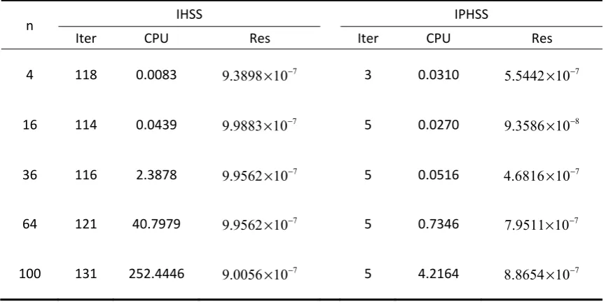
number of iterations. CPU is iterative time. The parameters are taken as _α ₌0.9. The preconditioned matrix P is selected as the diagonal matrix of the coefficient matrix A. Through the IPHSS algorithm we can get Table 1 as follows:

Table 1 Comparison of calculation results between IHSS and IPHSS method

n IHSS IPHSS

Iter CPU Res Iter CPU Res

4 118 0.0083 _{9.3898 10}_× −7 ₃ _0.0310 _{5.5442 10}_× −7

16 114 0.0439 _{9.9883 10}_× −7 ₅ _0.0270 _{9.3586 10}_× −8

36 116 2.3878 _{9.9562 10}_× −7 ₅ _0.0516 _{4.6816 10}_× −7

64 121 40.7979 _{9.9562 10}_× −7 ₅ _0.7346 _{7.9511 10}_× −7

100 131 252.4446 _{9.0056 10}_× −7 ₅ _4.2164 _{8.8654 10}_× −7

The numerical results in the analysis Table 1 show that the amplitude of the

number of iterative times for the IHSS iteration and the IPHSS iteration of the

(16)

very stable, but the number of iterations and times of the IPHSS iteration are far

smaller than that of the IHSS iteration, and the relative error of the IPHSS iteration is

also less than the relative error of the IHSS iteration.Not only that, it can be seen that

the gap between the iterative time of the IPHSS iterative method and the iteration time

of the IHSS iteration method is larger, as we can see the higher order of the matrix,

and thus the IPHSS iterative method for solving the generalized Lyapunov equation is

more effective than the IHSS iteration.

5 Conclusion

In this paper,a new method of solving the generalized Lyapunov equation by

PHSS iterative method is proposed and its convergence is proved. Then, the IPHSS

algorithm for solving the generalized Lyapunov equation is put forward, and the

convergence of the generalized Lyapunov equation is proved. Finally, a numerical

experiment is carried out to compare the new method with the existing methods. It is

found that compared with the IHSS iteration method, the IPHSS iteration method has

obvious improvement effect.

References

[1] Bai Z Z, Benzi M, Chen F. Modified HSS iteration methods for a class of complex symmetric linear system[J], Computing, 2010, 87(3-4): 93-111.

[2] Bai Z Z, Benzi M and Chen F. On preconditioned MHSS iteration methods for complex symmetric linear systems[J], Numerical Algorithms 56 (2011) 297–317.

[3] Bertaccini D. Ecient solvers for sequences of complex symmetric linear systems[J], Electronic Transactions on Numerical Analysis 18 (2004) 49–64.

[4] Feriani A A, Perotti F and Simoncini V. Iterative system solvers for the frequency analysis of linear mechanical systems[J], Computer Methods in Applied Mechanics and Engineering 190 (2000) 1719–1739.

[5] Wu S L, Li C X. A splitting method for complex symmetric indeﬁnite linear system[J], Journal of Computational and Applied Mathematics 313 (2017) 343-354.

[6] Wu S L, Li C X. Modiﬁed complex-symmetric and skew-Hermitian splitting iteration method for a class of complex-symmetric indenite linear systems[J], Numerical Algorithms, In press, DOI 10.1007/s11075-016-0245-1.

[7] Wu S L, Li C X. A splitting iterative method for the discrete dynamic linear systems[J], Journal of Computational and Applied Mathematics 267 (2014) 49-60.

(17)

[9] Bai Z Z, Golub G H, Pan J. Preconditioned Hermitian and skew-Hermitian splitting methods for non-Hermirian positive semidefinite linear systems[J], Numerische Mathematik, 2004, 98(1): 1-32.

[10]Bai Z Z, Golub G H, Li C. Convergence properties of preconditioned Hermitian and skew-Hermitian splitting methods for non-Hermitian positive semidefinite matrices[J], Mathematics of Computation, 2007, 76(257): 287-298.

[11]Yang A, An J, Yu J. A generalized preconditioned HSS method for non-Hermitian positive definite linear systems[J], Applied Mathematics and Computation, 2010, 216(6): 1715-1712.

[12]Xu Q.Q, Dai H. HSS iterative method for generalized Lyapunov equation [J], Journal of Applied Mathematics and Computational Mathematics , 2015, 29(4): 383-394.

[13]Bartels R H, Stewart G W. Solution of the matrix equation AX+XB=C[J], Communications of the ACM, 1972, 15(9): 820-826.

[14]Golub G H, Nash S, Van Loan C F. A Hessenber-Schur method for the matrix problem AX+XB=C[J], IEEE Transactions on Automatic Control, 1979, AC-24(6): 909-913.

[15]Lu A, Wachspress E L. Solution of Lyapunov equations by alternating direction implictiteration[J], Computers and Mathematics with Applications, 1991, 21(9): 43-58.

[16]Hu D Y, Reichel L. Krylov-Subspace methods for the Sylvester equation[J], Linear Algebra and Its Applications, 1992, 172(15): 283-313.

[17]Penzl T. A cyclic low-rank Smith method for large sparse Lyapunov equations[J], SIAM Journal on Scientific Computing, 1999, 21(4): 1401-1418.

[18]Li R. J, White J. Low-rank solution of Lyapunov equations[J], SIAM Journal on Matrix Analysis and Applications, 2004, 46(4): 693-713.