Very Low Rate Scalable Speech Coding through Classified Embedded Matrix Quantization

Volume 2010, Article ID 480345,13pages doi:10.1155/2010/480345

Research Article

Very Low Rate Scalable Speech Coding through Classified

Embedded Matrix Quantization

Ehsan Jahangiri

_{and Shahrokh Ghaemmaghami}

1_{Department of Electrical & Computer Engineering, Johns Hopkins University, Baltimore, MD 21218, USA} 2_{Department of Electrical Engineering, Sharif University of Technology, P.O. Box 14588-89694, Tehran, Iran}

Correspondence should be addressed to Ehsan Jahangiri,[email protected]

Received 21 June 2009; Revised 2 February 2010; Accepted 19 February 2010

Academic Editor: Soren Jensen

Copyright © 2010 E. Jahangiri and S. Ghaemmaghami. This is an open access article distributed under the Creative Commons Attribution License, which permits unrestricted use, distribution, and reproduction in any medium, provided the original work is properly cited.

This paper proposes a scalable speech coding scheme using the embedded matrix quantization of the LSFs in the LPC model. For an efficient quantization of the spectral parameters, two types of codebooks of different sizes are designed and used to encode unvoiced and mixed voicing segments separately. The tree-like structured codebooks of our embedded quantizer, constructed through a cell merging process, help to make a fine-grain scalable speech coder. Using an efficient adaptive dual-band approximation of the LPC excitation, where voicing transition frequency is determined based on the concept of instantaneous frequency in the frequency domain, near natural sounding synthesized speech is achieved. Assessment results, including both overall quality and intelligibility scores show that the proposed coding scheme can be a reasonable choice for speech coding in low bandwidth communication applications.

1. Introduction

Scalable speech coding refers to the coding schemes that reconstruct speech at different levels of accuracy or quality at various bit rates. The bit-stream of a scalable coder is com-posed of two parts: an essential part called thecoreunit and an optional part that includesenhancement units. The core unit provides minimal quality for the synthesized speech, while a higher quality is achieved by adding the enhancement units.

Embedded quantization, which provides the ability of successive refinement of the reconstructed symbols, can be employed in speech coders to attain the scalability property. This quantization method has found useful applications in variable-rate and progressive transmission of digital signals. The output symbol of an i-bit quantizer, in an embedded quantizer, is embedded in all output symbols of the (i+k )-bit quantizers, wherek≥1 [1]. In other words, higher rate codes contain lower rate codes plus bits of refinement.

Embedded quantization was first introduced by Tzou [1] for scalar quantization. Tzou proposed a method to achieve embedded quantization by organizing the threshold levels in the form of binary trees, using the numerical optimization of Max [2]. Subsequently, embedded quantization was

generalized to vector quantization (VQ). Some examples of such vector quantizers, which are based on the natural embedded property of tree-structured VQ (TSVQ), can be found in [3–5]. Ravelli and Daudet [6] proposed a method for embedded quantization of complex values in the polar form which is applicable to some parametric representations that produce complex coefficients. In the scalable image coding method introduced in [7] by Said and Pearlman, wavelet coefficients are quantized using scalar embedded quantizers.

Even though broadband technologies have significantly increased transmission bandwidth, heavy degradation of voice quality may occur due to the traffic-dependent variabil-ity of transmission delay in the network. A nonscalable coder operates well only when all bits, representing each frame of the signal, are recovered. Conversely, a scalable coder adjusts the need for optional bits, based on the data transmission quality, which could have significant impact on the overall performance of the reconstructed voice quality. Accordingly, only the core information is used for recovering the signal in the case of network congestion [8].

same data at different rates for users demanding the same voice signal [6]. This imposes an additional computational load on the server that may even result in congesting the network. A scalable coder can resolve this problem by adjusting the rate-quality balance and managing the number of optional bits allocated to each user.

A desirable feature of a coder is the ability to dynamically adjust coder properties to the instantaneous conditions of transmission channels. This feature is very useful in some applications, such as DCME (Digital Circuit Multiplica-tion Equipment) and PCME (Packet Circuit MultiplicaMultiplica-tion Equipment), in overload situations (too many concurrent active channels), “in-band” signaling, or “in-band” data transmission [9]. In case of varying channel condition that could lead to various channel error rates, a scalable coder can use a lengthier channel code, which in turn forces us to lower the source rate when bandwidth is fixed, to improve the transmission reliability. This is basically a tradeoffbetween voice quality and error correction capability.

Scalability has become an important issue in multimedia streaming over packet networks such as the Internet [9]. Several scalable coding algorithms have been proposed in literature. The embedded version of the G.726 (ITU-T G.727 ADPCM) [10], the MPEG-4 Code-Excited Linear Prediction (CELP) algorithm, and the MPEG-4 Harmonic Vector Excitation Coding (HVXC) are some of the standardized scalable coders [5]. The recently standardized ITU-T G.729.1 [11], an 8–32 kbps scalable speech coder for wideband telephony and voice over IP (VoIP) applications, is scalable in bit rate, bandwidth and computational complexity. Its bitstream comprises 12 embedded layers with a core layer interoperable with ITU-T G.729 [12]. The G.729.1 output bandwidth is 50–4000 Hz at 8 and 12 kbit/s and 50–7000 Hz from 14 to 32 kbit/s (per 2 kbit/s steps). A Scalable Phonetic Vocoder (SPV), capable of operating at rates 300–1100 bps, is introduced in [13]. The proposed SPV uses a Hidden Markov Model (HMM) based phonetic speech recognizer to estimate the parameters for a Mixed Excitation Linear Prediction (MELP) speech synthesizer [14]. Subsequently, it employs a scalable system to quantize the error signal between the original and phonetically-estimated MELP parameters.

In this paper, we introduce a very low bit-rate scalable speech coder by generalizing embedded quantization to matrix quantization (MQ), which is our main contribution in this paper. The MQ scheme, to which we add the embedded property, is based on the split matrix quantization (SMQ) of the line spectral frequencies (LSFs) [15]. By exploiting the SMQ, both the computational complexity and the memory requirement of the quantization are significantly reduced. Our embedded MQ coder of the LSFs leads to a fine-grainscalable scheme, as shown in the next sections.

The rest of the paper is organized as follows.Section 2

describes the method used to produce the initial codebooks for an SMQ. In Section 3, the embedded MQ of the LSFs is presented.Section 4is devoted to the model of the linear predictive coding (LPC) excitation and determination of the excitation parameters, including band-splitting frequency, pitch period, and voicing. Performance evaluation and some

experimental results using the proposed scalable coder are given inSection 5with conclusions presented inSection 6.

2. Initial Codebook Production for SMQ

In our implementation, the LSFs are used as the spectral features in an MQ system. Each matrix is composed of four 40 ms frames, each frame extracted using a hamming window of 50% overlap with adjacent frames, that is, a frame shift of 20 ms, sampled at 8 kHz. The LSF parameters are obtained from an LPC model of order 10, based on the autocorrelation method.

One of the problems we encounter in the codebook production for the MQ is the high computational complexity that usually forces us to use short training sequence or codebooks of small sizes. Although this is an one time process for the training of each codebook, it is time consuming to tune the codebooks by changing some parameters. In this case, writing fast codes (e.g., see [16]), exploiting a computationally modest distortion measure, and suboptimal quantization methods, make the MQ scheme feasible even for processors with moderate processing power. Multistage MQ (MSMQ) [17, 18] and SMQ [15] are two possible solutions to suboptimality in MQ. The Suboptimality of these quantizers mostly arises from the fact that not all potential correlations are used. By using SMQ, we achieve both a lower computational complexity for the codebook production and a lower memory requirement, as compared to a nonsplit MQ.

The LSFs are ideal for split quantization. This is because the spectral sensitivity of these parameters is localized; that is, a change in a given LSF merely affects neighboring frequency regions of the LPC power spectrum. Hence, split quantiza-tion of the LSFs cause negligible leakage of the quantizaquantiza-tion distortion from one spectral region to another [19].

The best dimensions of submatrices resulting from split-ting the spectral parameters matrix is addressed according to the empirical results given by Xydeas and Papanastasiou in [15]. It is shown that with four-frame length matrices of the spectral parameters and an LPC frame shift of 20 ms, the matrix quantizer operates effectively at 12.5 segments per second. This is comparable to the average phoneme rate and thus makes it possible to exploit most of the existing interframe correlation [15]. In addition, they found that the best SMQ performance at low rates was achieved when the spectral parameters matrixΓ10×4(assuming a 10×4 size for

each matrix of LSFs) was split into five equal dimension 2×4 size submatrices (Yi₎

2×4,i=1, 2,. . ., 5, given by

(Γl)10×4=

⎡ ⎢ ⎢ ⎢ ⎢ ⎢ ⎢ ⎢ ⎢ ⎢ ⎢ ⎢ ⎣

f1l f1l+1 f1l+2 f1l+3

f2l f2l+1 f2l+2 f2l+3

..

. ... ... ...

f9l f9l+1 f9l+2 f9l+3

f10l f10l+1 f10l+2 f10l+3

⎤ ⎥ ⎥ ⎥ ⎥ ⎥ ⎥ ⎥ ⎥ ⎥ ⎥ ⎥ ⎦

=

⎡ ⎢ ⎢ ⎢ ⎢ ⎢ ⎣

Y1_l

2×4

.. .

Y5_l

2×4

⎤ ⎥ ⎥ ⎥ ⎥ ⎥ ⎦, (1)

One of the most important issues in the design and oper-ation of a quantizer is the distortion metric used in codebook generation and codeword selection from codebooks during quantization. The distortion measure we use here is the squared Frobenius norm of weighted difference between the LSFs, defined as

D2Yi_l,Yi =Wlτ◦Wis,l◦(Yil−Yi)

2

F

=

2

m=1 4

t=1

w2τ(l+t−1)×w2s(l+t−1,i,m)

×f(li+−t1)−1×2+m−f(ti−1)×2+m

2

.

(2)

The operator ◦given in (2) stands for the Hadamard matrix product that is an element-by-element multiplication [20]. The input matrix,Yi_l, is considered as theith split of the matrix of the spectral parameters beginning with thelth frame. The reference matrix,Yi_{, in (2) can be a codeword}

of the ith split codebook. The time weighting matrix,Wl τ,

is to weight frames having a higher energy more than lower energy frames, as they are subjectively more important. Elements of thetth column (1 ≤ t ≤ 4) of this matrix are identical and are proportional to the power of the (l+t−1)th speech frame, given by

wτ(l+t−1)= n∈Φs

2_(n)

N

α/2

, 1≤t≤4,

Φ= {(l+t−2)×fsh + 1,. . ., (l+t−2)×fsh +N}, (3)

wheres(n) represents the speech signal, fsh andNstand for the frame shift and the frame length, respectively. According to [15],α=0.15 is a reasonable choice.

The definition of the spectral weighting matrix,Wi,l s, is

based on the weighting proposed by Paliwal and Atal [19]. The (m,t)th element of this matrix is proportional to the value of the power spectrum at corresponding LSFs of the frames included in the segment to be encoded, as

ws(l+t−1,i,m)=P

f(li+−t1)−1×2+m

0.15

,

1≤t≤4, 1≤m≤2, 1≤i≤5.

(4)

As we know, quantization of unvoiced frames can be done with a lower precision, as compared to voiced frames, with a negligible loss of quality. Accordingly, we exploit two types of codebooks: one for quantization of segments containing only unvoiced frames, Ψiuv , i = 1,. . ., 5, and

another for segments including either all voiced frames or a combination of voiced and unvoiced frames, Ψivuv, i =

1,. . ., 5. The unvoiced codebook, Ψiuv, is of smaller size

in comparison to the mixed voicing codebook, Ψivuv. This

selective codebook scheme leads to a classification-based quantization system that is known as classified quantizer ([3, pages 423-424]). This quantizer encodes the spectral parameters at different bit rates, depending on the voicing information, and thus leads to a variable rate coding system.

Table1: Number of bits allocated to the SMQ codebooks.

Codebook type

1st split

2nd split

3rd split

4th split

5th

split Total Mixed

voicing 10 10 10 9 8 47

Unvoiced 8 8 8 7 6 37

In this two-codebook design, an extra bit is employed for the codebook selection to indicate which codebook is to be used to extract the proper codeword.Table 1illustrates codebook sizes in our SMQ system. As shown, a lower resolution codebook is used for quantization of upper LSFs due to the lower sensitivity of the human auditory system (HAS) to higher frequencies. The bit allocation given inTable 1results in an average bit rate of 550 bps for representing the spectral parameters.

We designed codebooks of this split matrix quantizer, based on the LBG algorithm [21], using 1200 TIMIT files [22] as our training database. A sliding block technique is used to capture all interframe transitions in the training set. This is accomplished by using a four-frame window sliding over the training data in one-frame steps.

The centroid of the qth voronoi region is obtained by finding the derivatives of the accumulated distortion with respect to each element of the qth codeword of the SMQ codebooks and equating it to zero, leading to

∂

∂f(ti−1)×2+m

⎛ ⎜

⎝

l|Yi l∈Ri,q

D2Yi_l,Yi,q ⎞ ⎟ ⎠=0,

1≤t≤4, 1≤m≤2, 1≤i≤5,

(5)

whereRi,qrepresents the voronoi region of theqth codeword

of the ith split codebook that is, Yi,q_{, and l | Y}i l ∈ Ri,q represents frame indexes for whichYil belongs toRi,q.

Therefore, only the submatrices of the training data that fall into the voronoi region of theqth codeword are incorporated in the calculation of the centroid of the voronoi region. A closed form of the centroid calculation can be shown as

Yi,q₌ ⎛ ⎜

⎝

l|Yil∈Ri,q

Wi,l_◦Wi,l_◦Yi l

⎞ ⎟ ⎠ ÷

⎛ ⎜

⎝

l|Yil∈Ri,q

Wi,l_◦Wi,l ⎞ ⎟ ⎠,

(6)

where

Wi,l_=Wl

τ◦Wis,l (7)

and the operator÷ denotes an element-by-element matrix division.

the centroid. Our solution to preserve stability of the LPC synthesis filters is to put all five generated codewords into a 10×4 matrix and then sort each column of not yet ascended order columns of the reproduced spectral parameters matrix across all 5 codewords in ascending order. However, the resulting synthesis filters might become marginally stable due to the poles located too close to the unit circle. The problem is aggravated in fixed-point implementation, where a marginally stable filter can actually become unstable after quantization and loss of precision during processing. Thus, in order to avoid sharp spectral peaks in the spectrum that may lead to unnatural synthesized speech, bandwidth expansion through modification of the LPC vectors is employed. In this case, each LPC filter coefficient, ai, is

replaced by aiγi, for 1 ≤ i ≤ 10, where γ = 0.99. This

operation flattens the spectrum, especially around formant frequencies. Another advantage of the bandwidth expansion is to shorten the duration of the impulse response of the LPC filter, which limits the propagation of channel errors ([8, page 133]).

The next section introduces the method to construct the tree structured codebooks for the embedded quantizer, using the initial codebooks designed in this section.

3. Codebook Production for Embedded

Matrix Quantizer

Consider the initial codebookΨgenerated using the SMQ method described in the preceding section. For notational convenience, we have dropped the superscript “i” and subscripts “uv” and “vuv”. The codewords of the codebook

Ψare denoted by

Ψ=Y0,Y1,. . .,YNt−1

, (8)

whereNtis the number of codewords or the codebook size.

We organize these initial codewords in a tree structure to determine the internal codewords of the constructed tree, such that each internal codeword is a good approximation to its children. Codewords emanating from an internal codeword are called children of that internal codeword. In a binary tree, each internal codeword has two children. The index length of each initial codeword determines the depth of the tree.Figure 1illustrates a binary tree of depth three. We place initial codewords at the leaves of the tree. Hence, each terminal node on the tree corresponds to a particular initial codeword. To produce a tree structure having the embedded property, symbols at lower depths (farther from the leaves) must be the refined versions of the symbols at higher depths (closer to the leaves). One of the methods that can be used to incorporate the embedded property into the tree is cell-merging or region-merging method. A cell-merging tree is formed by cell-merging the Voronoi regions in pairs and allocating new centroids to these larger encoding areas. Merging two regions can be interpreted as erasing the boundary between the regions on the Voronoi diagram [23]. Now the problem is to find the regions that should be merged to minimize the distortion of the internal codewords in their Voronoi regions. By merging the proper codewords,

0

0

1

0 1

0 1

0

0 1 1 0 1 0 1

1

{0, 0, 0} {0, 0, 1} {0, 1, 0} {0, 1, 1} {1, 0, 0} {1, 0, 1} {1, 1, 0} {1, 1, 1} Figure1: A depth-3 tree structure for an embedded quantization scheme. Indexes of terminal nodes, corresponding to initial code-words, are indicated below the nodes.

the constructed tree makes a fine-grain scalable system. A simple solution to this problem is to exhaustively evaluate all possible index assignment sequences for the leaves of the tree and find the corresponding tree for each sequence, and then keep the sequence that leads to the lowest total accumulated distortion (TAD) on the training sequenceT=

{Y1,Y2,. . .,YK}for all depths, as

TAD=

td

d=1

AD(d)_{, (9)}

where td = log₂(Nt) is the depth of the tree and AD(d) is

the sum of the accumulated distortions for all codewords in depthdon the training sequenceT, defined as

AD(d)=

2d₋₁

m=0

ADYd m,

ADYd m=

l|Yl∈Rdm

DYl,Ydm , l∈ {1, 2,. . .,K},

(10)

where Rd

m represents the Voronoi region of Ydm and the

metric D(Yl,Ydm) is the distance between Yl and Ydm. It is

worth mentioning that we have 2d _{codewords at depth d.}

In (10), the summation is over all valid ls, that is, l ∈ {1, 2,. . .,K}, for whichYlbelongs to the voronoi regionRdm.

According to [4], the total number of index assignment sequences for the leaves of the tree that need to be evaluated in an exhaustive search to minimize (9) is given by

Ω=

log2(Nt/2)

i=0

Nt/2i

! 2((Nt/2i+1)!)2

2i

. (11)

This number becomes quite large even for moderate values ofNt. Hence, this simple solution cannot be used in practice

due to its prohibitively high complexity.

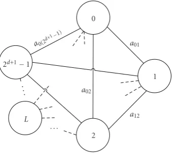
Hence, in order to make the merging process feasible, we need to use more computationally efficient methods. A simple suboptimal solution is to merge the pairs of regions at depthd+ 1 that only minimize the accumulated distortion in depthd. In this method, the total accumulated distortion on the designated cell-merging tree, defined in (9), may not come to its minimum. To choose proper pairs of the Voronoi regions to merge at depthd+ 1, we may generate an undirected graph with 2d+1_{nodes, labeled from 0 to 2}d+1_−1,

2d+1₋₁ a0(2d

+1−1)

L

2

1 0

a02

a12 a01

._. .

. . .

Figure2: The graph for codewords at depthd+ 1. Arc valueai j

is determined based on the encountered distortion resulting from mergingith andjth codewords at depthd+ 1.

one particular codeword at depthd+ 1 and the arc between every two nodes is the value of accumulated distortion on the training sequence for the codeword resulting from merging two codewords at two ends of the arc.

The problem of finding proper regions to merge is similar to a complete bipartite matching problem ([24, page 182]). In fact, we must select a subset of the graph illustrated in

Figure 2that minimizes the accumulated distortion in depth d,while no two arcs are incident to the same node and all of the nodes are matched. Some methods to solve this problem are presented in [24] that offer a computational complexity of O(n3_{), where n is the number of nodes in the graph.}

However, we used the suboptimal method proposed by Chu in [4] to reduce the merging processing time, which worked well in our implementation. In this method, we sort arc values in ascending order, select arcs with lower values, and remove arcs ending at nodes belonging to the arcs already selected. Therefore, no sharing occurs between Voronoi regions at depthd, which is a necessary characteristic for the constructed tree. The select-remove procedure is continued until a complete matched graph is achieved.

In the following part of this section, we propose four types of distortion criteria to attribute to arc values in the merging process and give details of a comparative assessment.

Consider the training sequenceT = {Y1,Y2,. . .,YK},

where K is a large number. And, suppose Rr and Rs are

the Voronoi regions of codewordsYrandYsat depthd+ 1,

respectively. ConsiderYrsas the mother ofYrandYsat depth d. The mother codewordYrsis a codeword for representing

bothRrandRsVoronoi regions. We estimate a measure of

the accumulated squared distortion for the training matrices that fall into the Voronoi region ofYrsat depthd, that is,{for

all Yl | Yl ∈ Rrs}, according to the accumulated squared

distortions of the codewords Yr and Ys. For the Voronoi

region ofYrs,Rrs, we have

Rrs≈Rr∪Rs, Rr∩Rs=∅, (12)

where the approximation in (12) arises from the fact that an input matrix which hasYr orYsas its nearest neighbor

codeword at depth d+ 1 may no longer have Yrs as its

nearest neighbor codeword at depthd([3, page 415]). The approximation in (12) turns into equality, when the Voronoi regions of codewords Yr andYsare determined through a

tree search, as

Rrs=Rr∪Rs. (13)

Hereafter, we assume that (13) is satisfied, even if no tree search is made. We define the sum of element-by-element squared weights for the training matrices that fall into Rr

andRsVoronoi regions, as

W2r =

l|Yl∈Rr

Wl◦Wl,

W2

s=

l|Yl∈Rs

Wl_◦Wl_.

(14)

We define the accumulated squared weighted distortion for the Voronoi region of codewordYrsat depthd, as

AD2rs=

l|Yl∈Rrs

Wl◦Yl−Yrs

2

F. (15)

By taking the derivatives of this accumulated distortion with respect to each element ofYrs, and equating them to zero, the

optimumYrsis obtained, as

Yrs= ⎛

⎝

l|Yl∈Rrs

Wl◦Wl◦Yl ⎞ ⎠ ÷

⎛

⎝

l|Yl∈Rrs

Wl◦Wl

⎞ ⎠

=W2r◦Yr+W2s◦Ys ÷

W2r+W2s

.

(16)

We decompose (15) into two Voronoi regionsRrandRs, as

AD2rs=

l|Yl∈Rrs

Wl◦Yl−Yrs

2

F

=

l|Yl∈Rr

Wl_◦Y

l−Yrs

2

F

+

l|Yl∈Rs

Wl◦Yl−Yrs

2

F=D

2

r+ D2s,

(17)

where

D2r=

l|Yl∈Rr

Wl◦Yl−Yrs

2

F

=

l|Yl∈Rr

Wl_◦Y

l

2

F−2×

l|Yl∈Rr

Wl_◦Wl_◦Y l◦Yrs

+

l|Yl∈Rr

Wl◦Yrs

2

F,

and · stands for the sum of all elements of the operand matrix. We also have

AD2r =

l|Yl∈Rr

Wl◦Yl

2

F−

W2r◦Yr◦Yr,

l|Yl∈Rr

Wl◦Wl◦Yl◦Yrs=W2r◦Yr◦Yrs,

l|Yl∈Rr

Wl◦Yrs

2

F=

W2r◦Yrs◦Yrs.

(19)

By substituting (19) into (18) we get

D2r=AD2r+W2r◦Yr◦Yr−2×W2r◦Yr◦Yrs

+W2

r◦Yrs◦Yrs

=AD2

r+ W2 r◦

Yr−Yrs ◦2

,

(20)

where (·)◦2 denotes an element-by-element square of the operand matrix. By replacingYrsfrom (16) into (20), we get

D2

r =AD2r+ W2

r◦

Yr−Ys ◦W2s÷

W2

r+W2s ◦2

.

(21)

Similarly, we can compute D2s, as

D2_s =AD2_s+W2

s◦

Yr−Ys ◦W2r÷

W2

r+W2s ◦2

.

(22)

Finally, the accumulated squared weighted distortion for the Voronoi region of the codewordYrs at depthdcan be

simplified to

AD2

rs=D2r+ D2s =AD2r+ AD2s

+Yr−Ys ◦2

◦W2

r◦W2s

÷W2

r+W2s,

(23)

where, in the no-weighting case, it reduces to

AD2_rs=AD2_r+ AD2_s+ nrns

nr+ns

Yr−Ys

2

F (24)

In (24),nrandnsare the number of training matrices that fall

into the Voronoi region ofYr andYs, respectively. Equation

(23) in the case of no-weighting and vector codewords reduces to the Equitz’s formula in [23].

Therefore, by considering the term added to the accu-mulated distortions of children codewords at the right side of (23) or (24), as the value of the arc between nodes corresponding to children codewords, and then selecting a complete matching subset of the graph so that the sum of its arcs is minimized, the proper codewords for merging can be determined. Generalizing Chu’s distortion measure [4] to our case results in the arc value of

ars=

W2r

÷W2r+W2s

◦Yr−Yrs ◦2

+W2s

÷W2r+W2s

◦Ys−Yrs ◦2

.

(25)

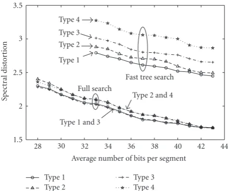
1.5 2 2.5 3 3.5

Spect ral dist o rt ion

28 30 32 34 36 38 40 42 44

Average number of bits per segment Type 1 and 3

Type 2 and 4 Full search

Fast tree search Type 1 Type 2 Type 3 Type 4 Type 1 Type 2 Type 3 Type 4

Figure3: Spectral Distortion (SD) in dB versus average number of bits per segment for four types of accumulated distortion measures.

Equation (25) in the no-weighting case reduces to

ars= nr

nr+ns

Yr−Yrs

2

F+

ns

nr+ns

Ys−Yrs

2

F (26)

where

Yrs=

nrYr+nsYs

(nr+ns) .

(27)

In case the rth codeword and the sth codeword are to be merged, the accumulated weighting for the codeword Yrs

(that is an average over children codewords,Yr andYs, as

mentioned in (16) and (27) for weighting and no-weighting conditions, respectively) is

W2rs=W2r+W2s, (28)

where it turns intonrs=nr+nsin the case of no-weighting.

By continuing the cell-merging procedure (allocating distortion criterion to arcs, and then selecting a matched graph) for the codewords of all depths, we construct the tree-structured codebooks corresponding to each initial codebook. One of the most effective and readily available techniques for reducing the search complexity is to rely on the tree-structured codebooks in our embedded quantizer design.Figure 3illustrates spectral distortion (SD) versus the average number of bits per segment in both full and fast tree searches for tree-structured codebooks constructed by exploiting four types of accumulated distortion measures. Types 1, 2, 3, and 4 distortion measures correspond to distortion criteria based on (23), (24), (25), and (26), respectively.

Table2: The bit allocation used for embedded quantization at different rates. UV and VUV correspond to unvoiced and mixed voicing codebooks, respectively.

Average bits per segment

No. of bits for No. of bits for No. of bits for No. of bits for No. of bits for

representing representing representing representing representing

LSF1 & LSF2 LSF3 & LSF4 LSF5 & LSF6 LSF7 & LSF8 LSF9 & LSF10

VUV UV VUV UV VUV UV VUV UV VUV UV

43 10 8 10 8 10 8 9 7 8 6

42 10 8 10 8 10 8 9 7 7 5

41 10 8 10 8 10 8 8 6 7 5

40 10 8 10 8 9 7 8 6 7 5

39 10 8 9 7 9 7 8 6 7 5

38 9 7 9 7 9 7 8 6 7 5

37 9 7 9 7 9 7 8 6 6 4

36 9 7 9 7 9 7 7 5 6 4

35 9 7 9 7 8 6 7 5 6 4

34 9 7 8 6 8 6 7 5 6 4

33 8 6 8 6 8 6 7 5 6 4

32 8 6 8 6 8 6 7 5 5 3

31 8 6 8 6 8 6 6 4 5 3

30 8 6 8 6 7 5 6 4 5 3

29 8 6 7 5 7 5 6 4 5 3

28 7 5 7 5 7 5 6 4 5 3

27 7 5 7 5 7 5 6 4 4 2

is represented inTable 2 by lowering the rate, the amount of bits allocated to high-frequency LSFs is reduced first, due to their lower perceptual importance. By decreasing one bit, we select a codeword from a lower depth stage of the tree-structured codebook. Each step of bit reduction inTable 2is equivalent to 12.5 bps decrease in bit rate.

The Spectral Distortion (SD) is applied to 4 minutes of speech utterances outside the training set. As depicted in Figure 3, in the case of full search, type 1 and type 3 distortion measures perform almost similarly and a little better than their unweighted versions (types 2 and 4). Indeed, full codebook search results in the same performance for these four types of measures at full resolution, because all the four types of trees have the same terminal nodes. Although the type 3 measure performs better than the type 2 measure in full search, it is outperformed by types 1 and 2 distortion measures in the fast tree search. This behavior comes from the fact that equality (13) is satisfied for the fast tree search.

It is clear from Figure 3 that the fast tree search does not necessarily find the best matched codeword. Generally speaking, it may be thought that there should be a slight difference between the spectral distortions in full search and fast tree search; nevertheless, we believe this relatively considerable difference, which we see in Figure 3, is due to the codebook structures having matrix codewords.

4. Adaptive Dual-Band Excitation

Multiband excitation (MBE) was originally proposed by Griffin and Lim and was shown to be an efficient paradigm for low rate speech coding to produce natural sounding speech [25]. The original MBE model, however, is inappli-cable to speech coding at very low rates, that is, below 4 kbps, due to the large number of frequency bands it employs. On the other hand, dual-band excitation, as the simplest possible MBE model, has attracted lots of attention by the research community [26]. It has been shown that most (more than 70%) of the speech frames can be represented by only two bands [26]. Further analysis of the speech spectra revealed that the low frequency band is usually voiced, where the high-frequency band usually contains a noise-like signal (i.e., unvoiced) [26]. In our coding system, we use the dual-band MBE model proposed in [27], in which the two bands join at a variable frequency determined based on the voicing characteristics of speech signals on a frame-by-frame basis in the LPC model. For convenience, we have quoted the main idea of this two-band excitation model from [27] below.

Impulse generator with

LPC-10 excitation signal Pitch period

Low-pass filter

Transition frequency

High-pass filter White noise

generator

Gain

Synthesis filter

Synthesized speech

LPCs

Figure4: Block diagram of the adaptive dual-band synthesizer. Transition frequency controls cutofffrequency of low-pass and high-pass filters.

of the signal change. Figure 4 shows the block diagram of the two-band synthesizer where near zero values for transition frequency mean pure unvoiced, near 4 KHz values mean pure voiced, and mid values mean mixed patterns of voiced and unvoiced. Given a transition frequency, an artificial excitation is constructed by adding a periodic signal located at the low band, that is, below transition frequency, and a random signal at the high band, that is, above transition frequency. For the voiced part, the excitation pulse of the LPC-10 coder is used as the pulse-train generator [28]. This excitation signal improves the quality of the synthesized speech over the simple rectangular pulse train. This excitation pulse is shown inFigure 5.

The transition frequency is computed from the spectrum of the LPC residual for each frame of the signal using a periodicity measure, which is based on the flatness of the instantaneous frequency (IF) contour in the frequency domain. For IF estimation in the frequency domain, which gives the pitch period when the frame is voiced, we use a spectrogramtechnique that employs a segment-based analysis using an appropriate window in the frequency domain [29]. Pay attention that this windowing process is different from the one we used in the time domain. The windowing in the time domain is same as the one we used inSection 2. Here, the windowing is performed in the frequency domain using aHanningwindow

S(k,l)=

M12

M1

r=1

E(k+r)e−j(2πr/M2)l_w(r)

2

,

k=1, 2,. . .,N

2,l=1, 2,. . .,M1,

(29)

where E(k) represents a filtered version of the spectrum magnitude of the residual signal,N is the total number of samples in each frame of the speech signal which is 320 here,

M1 = min{N/2,k+ M} −k, M < M2 < N/2, S(k,l) in

thelth spectrogram coefficient,M2 in the number of DFT

points which is 64 here,Mis the predefined window length which is 32 here, and w(r), r =1, 2,. . .,M1, is a Hanning

window in the frequency domain. As is evident, as long as

k+M < N/2,M1equalsM. The peak of the spectrogram,

−400

−300

−200

−100 0 100 200 300 400

A

m

plitude

0 5 10 15 20 25 30 35 40

n(index)

Figure5: One excitation pulse of the LPC-10 coder [28].

S(k,l),l=1, 2,. . .,M1, gives the IF of the spectrumE(k)

ξ(k)=max{S(k,l)}, k=1, 2,. . .,N

2, (30)

whereξ(k) represents IF of the spectrum over frequencies from 0 toFs/2, whereFsis the sampling frequency which is

8 kHz in our designated coder.

The transition frequency, ftrans, which specifies a change

in the spectrum characteristics from periodic to random, is obtained through measuring theflatnessofξ(k) in a number of subbands,nb. This is formulated as

ζj=exp

logκ2j

κ2

j

, j=1, 2,. . .,nb, (31)

where j is the subband index, κ2

j = {ξ2j1ξ2j2· · · }, and

the vector κj = {ξj1ξj2· · · } is the jth part of ξ(k), k

= 1, 2,. . .,N/2, located in the jth band, whose flatness is represented byζ(j). The bar over the vectorκ2

jstands for the

mean of this vector.

As evident, 0 < ζ ≤1, which is used as an indication of flatness, where 1 is for an absolutely-flat vector (ξj1=ξj2 =

· · ·). ftrans, is then calculated through comparingζ(j) with

the threshold th, as

ftrans=j0 Fs

2nb

−1 0 1

(kHz)

X

(

f

)

0.5 1 1.5 2 2.5 3 3.5 4 (a)

0 0.2 0.4

IF

0.5 1 1.5 2 2.5 3 3.5 4 (kHz)

(b)

0 40 ms

(c)

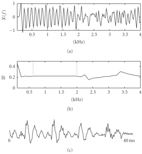
Figure6: IF based analysis of a mixed-excitation speech signal: (a) absolute value of LPC residual where its mean value is removed, (b) IF contour over frequency domain, and (c) speech signal waveform. The portion of the IF contour between vertical lines is used to compute the fundamental frequency [27].

where j0 =min{j | ζ(j) < th}, that means the minimum

value ofjfor whichζ(j)<th.

The threshold is calculated based on the mean of the spectrum flatness within a certain band, averaged over a number of previous frames composed of voiced and unvoiced frames [27]. In this way, the spectrum is assumed to be periodic at frequencies belowftrans, and it is considered

random at frequencies over ftrans, with a resolution specified

bynb.

The fundamental frequency, f0, is computed using f0 =

Fs/T = Fs/(IF× N) where IF is the mean value of the

IF contour within a certain band below 1 kHz regardless of its voicing status, as illustrated in Figure 6, where a mixed speech signal and its corresponding IF curve are shown. The degree of voicing, or periodicity, is determined by the transition frequency. A low ftrans means that the

periodic portion of the excitation spectrum is dominated by the random part and vice versa. For this reason, the accuracy in pitch detection during unvoiced periods, which is intrinsically ambiguous, is insignificant and noneffective in naturalness. A detailed description of this dual-band excitation method can be found in [27] by Ghaemmaghami and Deriche.

We exploit interframe correlation between adjacent frames (in each segment of four frames) to efficiently encode gain, pitch period, and transition frequency using a 4 × 1 dimension vector quantization for each set of excitation parameters. Codebooks for these parameters are built using the LBG algorithm by a simple norm-2 distortion measure. The training vectors are produced using 1200

Table3: Bits allocation for pitch, transition frequency, and gain codebooks.

Codebook type Pitch Transition Frequency Gain Total No. of bits allocated 11 9 7 27

Table 4: Spectral dynamics and spectral distortion of matrix quantization versus vector quantization at the same rate.

Average number of bits per

segment of four frames 43 38 33 ASE for original speech 6.57 6.57 6.57 ASE for MQ 6.21 6.15 6.11 ASE for MQ with segments

junction smoothing 6.08 6.02 5.97 ASE for VQ at the same rate

as MQ 6.56 6.54 6.43

ASD for MQ 1.65 1.75 2.05 ASD for MQ with segments

junction smoothing 1.63 1.72 2.01 ASD for VQ at the same

rate as MQ 2.50 2.68 3.02

speech files from TIMIT.Table 3 illustrates the number of bits we assign to the codebooks of these parameters. This bit allocation scheme and the one extra bit employed for the codebook type selection lead to a rate of 350 bps ((27 + 1)/80 ms) for encoding the excitation parameters, and the total rate of 900 bps (350 + 550) in full resolution embedded quantization of spectral parameters. Reducing the number of bits for representing pitch and the transition frequency severely affects the speech quality. Since, we encode these excitation parameters using a fixed number of bits, given in

Table 3, at any rate selected.

5. Performance Evaluation and Experiments

5.1. Spectral Dynamics of MQ versus VQ. The dynamics of the power spectrum envelope play a significant role in the perceived distortion [30]. According to Knagenhjelm and Kleijn [30], smooth evolution of the quantized power spectrum envelope leads to a significant improvement in the performance of the LPC quantizers. To evaluate the spectral evolution, the spectral difference between adjacent frames is used which is given by

SE2

i =

1 2π

+π

−π !

10 log₁₀(Pi+1(w))−10 log10(Pi(w)) "2

dw,

(33)

wherePi(w) indicates the power spectrum envelope of the ith frame.Table 4compares average spectral evolution (ASE) and average spectral distortion (ASD) of the embedded matrix quantizer (produced by type 1 distortion criterion) versus VQ for three different numbers of bits assigned to each segment of spectral parameters.

0 1 3 2 4 5

(MOS)

700 800 900

(bps)

Figure7: MOS score at three different rates. Scores of 2.71, 2.82, and 2.92 are achieved for 700, 800, and 900 bps, respectively.

have smooth spectral trajectories, thus the averaging process over the matrices results in codewords having relatively smooth spectral dynamics. This is while codewords of the VQ are obtained by averaging over a set of single frame input vectors and not a trajectory of spectral parameters like MQ. This results in better performance of the MQ over the VQ, in terms of spectral dynamics, as confirmed by experimental results given in Table 4. According to this table, the MQ yields both smoother spectral trajectories and lower average spectral distortions, as compared to the VQ at a same rate.

To improve the performance of the MQ, we use simple spectral parameter smoothing at the junction of codewords selected in consecutive segments. In this smoothing method, we replace the first column of the selected minimum distortion codeword by a weighted mean of the first column of the currently selected codeword and the last column of the previously selected codeword. Weighting used for the first column of the recent codeword is 0.75 and for the last column of the previously selected codeword is 0.25. In this smoothing method, the ascending order of the LSFs is guaranteed.

5.2. Intelligibility and Quality Assessment. We use the ITU-T P.862 PESQ standard [31] to compare the quality of synthesized speech at various bit rates. The PESQ (Perceptual Evaluation of Speech Quality) score ranges from −0.5 to 4.5, with 1 for a poor quality and 4 denoting a high quality signal. The PESQ, which is an objective measure to evaluate speech quality, correlates well with subjective test scores at mid and above mid bit rates. However, PESQ does not give a reasonable estimate of MOS at low bit rates. Therefore, we have just used PESQ for quality comparison between various bit rates and not for an estimate of MOS. The material used for the PESQ test is a 3-minute long speech signal outside the training set.Table 5illustrates the PESQ score at different rates of the scalable coder for full and fast tree searches, where the tree-structured codebook is produced using type 1 distortion criterion.Figure 7shows the results of the MOS subjective quality test [32] at three different rates exploiting a tree-structured codebook identical to the one used in PESQ tests using a full search for choosing codewords. The MOS test was conducted by asking 24 listeners to score 3 stimuli sentences.

We also conducted the MUSHRA ITU-R recommenda-tion BS.1534-1 test [33] at the same bit rates and with the

0 20 40 60 80 100

(MUSHRA)

700 800 900

(bps)

Figure8: MUSHRA score at three different rates. Scores of 38, 40, 43 are achieved for 700, 800, and 900 bps, respectively.

Table5: PESQ scores at different rates.

Bit rate PESQ score PESQ score (full search) (tree search)

900 2.512 2.331

850 2.468 2.298

800 2.447 2.293

750 2.437 2.28

700 2.38 2.24

No-quantization case 2.651

same codebooks (Figure 8). MUSHRA stands for “MUltiple Stimuli with Hidden Reference and Anchor” and is a method for subjective quality evaluation of lossyaudio compression algorithms. MUSHRA listening test is a 0–100 scale that is particularly suited to compare high quality reference sounds with lower quality test sounds. Thus, test items where the test sounds have a near-transparent quality or where the reference sounds have a low quality should not be used. For the MUSHRA test we used the MUSHRAM interface given in [34] and asked 10 subjects to help us in the experiment.

As it is clear in Figures 7and 8, the quality difference between these three rates is relatively small, consistent with the fine-granularity property. In some speech samples the quality difference at different rates was almost imperceptible. The results shown in these figures are achieved by doing the test over a variety of samples and taking the average over the scores.

Figure 9 illustrates spectrograms for a sample speech utterance from TIMIT, uttered by a male speaker, “Do not ask me to carry an oily rag like that,” at different rates. As shown in the figure, details of the spectrograms tend to disappear at lower rates. This figure also reveals that the difference between the original and the synthesized speech spectra mainly stems from the inaccuracy of the dual-band approximation of the LPC excitation, as compared to the effect of the LSF quantization.

In addition to the quality test, we conducted the diagnos-tic rhyme test (DRT) [35] to measure the intelligibility of the synthesized speech.Table 6gives results of this test at three different rates.

0 500 1000 1500 2000 2500 3000 3500 4000

Fre

q

u

en

cy

0 0.2 0.4 0.6 0.8 1 1.2 1.4 1.6 1.8 2 2.2 Time

(a) Original Speech

0 500 1000 1500 2000 2500 3000 3500 4000

Fre

q

u

en

cy

0 0.5 1 1.5 2

Time

(b) Synthesized speech without parameter quantization

0 500 1000 1500 2000 2500 3000 3500 4000

Fre

q

u

en

cy

0 0.5 1 1.5 2

Time

(c) Synthesized speech at average bit rate of 825 bps

0 500 1000 1500 2000 2500 3000 3500 4000

Fre

q

u

en

cy

0 0.5 1 1.5 2

Time

(d) Synthesized speech at average bit rate of 762 bps

0 500 1000 1500 2000 2500 3000 3500 4000

Fre

q

u

en

cy

0 0.5 1 1.5 2

Time

(e) Synthesized speech at average bit rate of 700 bps

Table6: DRT assessment results.

Bit-rate 900 800 700

Voicing 100 100 100

Nasality 67 62 56

Sustention 78 73 70

Sibilation 87.5 87.5 85

Graveness 100 100 100

Compactness 100 87.5 87.5

Total 89 85 83

store the internal codewords, in addition to the memory required to storeNtcodewords of the initial codebook placed

on the leaves of the tree. The total number of noninternal codewords is given by

1 + 2 + 22_{+· · ·+ 2}(log2(Nt))−1=₂(log2(Nt))−₁=_N

t−1.

(34)

Thus, the total amount of memory required for the embedded quantizer is slightly less than twice of the memory used for the initial codebooks. In the applications based on fast tree-structured search, there is no need to have internal codewords at the decoder. This is while the internal codewords must be available in both coder and decoder in an embedded quantization scheme ([3, page 413]).

The total memory required to store spectral parameters for the designated classified embedded SMQ is computed as

Memory

=

⎛ ⎝5

i=1

2Ntvuv,i−1 +

5

i=1

2Ntuv,i−1 ⎞

⎠_×8=76720, (35)

where Ntvuv,iand Ntuv,i denote sizes of ith initial split

codebooks corresponding to mixed voicing and unvoiced codebooks, respectively. And, in the case of the nonsplit embedded quantizer of the same resolution, the amount of memory is given as

Memory

=

⎛ ⎝ ⎛ ⎝₂

⎡ ⎣5

i=1

Ntvuv,i

⎤ ⎦₋₁

⎞ ⎠₊

⎛ ⎝₂

⎡ ⎣5

i=1

Ntuv,i

⎤ ⎦₋₁

⎞ ⎠ ⎞ ⎠_×40

≈1.13×1016_.

(36)

Hence, the embedded SMQ proposes a memory requirement that is much lower than that of a nonSMQ of the same resolution. This confirms a proper selection of the SMQ for our embedded matrix quantizer in the sense of both the computational complexity and size of the memory.

6. Conclusion

In this paper, which was a detailed version of [36], we have introduced a very low rate scalable speech coder with 80 ms coding delay, using classified embedded matrix quantization

and adaptive dual-band excitation. Although the delay is relatively high with respect to many standardized coders, it is still suitable for some applications, since a delay as high as 250 ms has found to be tolerable for some practical applications according to [37–39]. The transition frequency of the dual-band excitation model is determined based on the evaluation of flatness of the instantaneous frequency contour in the frequency domain. A cell-merging process is applied to the initial codebooks of the SMQ scheme to organize code-words into a tree-structure. The natural embedded property of the constructed tree codebooks helped to build a fine-grain scalable coder operating in the range of 700–900 bps at 12.5 bps steps. It is obvious that a same cell merging process can be applied to larger size initial codebooks in order to get a wider range of bit rate operation. Our intention of testing the bit range of 700–900 was just to evaluate the granularity of the designed embedded quantizer. Four types of distortion measures to assign to the arc values of the initial graph in the merging process, in both full and fast-tree searches, have been introduced and assessed comparatively. Interframe correlation between adjacent frames is exploited to efficiently encode gain, pitch, and the transition frequency using the VQ method. Better performance of the proposed embedded matrix quantizer in comparison with the VQ, at the same bit rate, has been confirmed, in terms of both spectral dynamics and spectral distortion. Speech quality assessment and DRT comparison of the synthesized speech at different rates show that the proposed scalable coding system has the property of fine-granularity.

Acknowledgment

The authors want to express their thankfulness to Dr. Wai C. Chu and also our friend Tim Han for reviewing this paper several times and making valuable comments and suggestions.

References

[1] K.-H. Tzou, “Embedded Max quantization,” inProceedings of IEEE International Conference on Acoustics, Speech and Signal Processing (ICASSP ’86), pp. 505–508, Tokyo, Japan, 1986. [2] J. Max, “Ouantization for minimum distortion,”IEEE

Trans-actions on Information Theory, vol. 6, pp. 7–12, 1960. [3] A. Gersho and R. M. Gray, Vector Quantization and Signal

Compression, Kluwer Academic Publishers, Dordrecht, The Netherlands, 1992.

[4] W. C. Chu, “Embedded quantization of line spectral frequen-cies using a multistage tree-structured vector quantizer,”IEEE Transactions on Audio, Speech and Language Processing, vol. 14, no. 4, pp. 1205–1217, 2006.

[5] W. C. Chu, “A scalable MELP coder based on embedded quantization of line spectral frequencies,” inProceedings of International Symposium on Intelligent Signal Processing and Communication Systems (ISPACS ’05), pp. 29–32, Hong Kong, December 2005.

[6] E. Ravelli and L. Daudet, “Embedded polar quantization,”

IEEE Signal Processing Letters, vol. 14, no. 10, pp. 657–660, 2007.

Transactions on Circuits and Systems for Video Technology, vol. 6, no. 3, pp. 243–250, 1996.

[8] W. Chu,Speech Coding Algorithms: Foundation and Evolution of Standardized Coders, John Wiley & Sons, New York, NY, USA, 2003.

[9] O. Hersent, J. P. Petit, and D. Gurle,Beyond VoIP Protocols: Understanding Voice Technology and Networking Techniques for IP Telephony, John Wiley & Sons, New York, NY, USA, 2005. [10] ITU, “5−, 4−, 3−, and 2-Bits Sample Embedded Adaptive

Dif-ferential Pulse Code Modulation (ADPCM)—Recommend,” G.727, Geneva, Switzerland, 1990.

[11] ITU-T Rec. G.729.1, “G.729-based embedded variable bit-rate coder: an 8-32 kbit/s scalable wideband coder bitstream interoperable with G.729,” May 2006.

[12] ITU-T Rec. G.729, “Coding of Speech at 8 kbit/s Using Conjugate Structure Algebraic Code Excited Linear Prediction (CSACELP),” March 1996.

[13] A. McCree, “A scalable phonetic vocoder framework using joint predictive vector quantization of melp parameters,” in

Proceedings of IEEE International Conference on Acoustics, Speech and Signal Processing (ICASSP ’06), vol. 1, pp. 705–709, Toulouse, France, May 2006.

[14] L. M. Supplee, R. P. Cohn, J. S. Collura, and A. V. McCree, “MELP: the new federal standard at 2400 bps,” inProceedings of IEEE International Conference on Acoustics, Speech and Signal Processing (ICASSP ’), vol. 2, pp. 1591–1594, Munich, Germany, April 1997.

[15] C. S. Xydeas and C. Papanastasiou, “Split matrix quantization of LPC parameters,”IEEE Transactions on Speech and Audio Processing, vol. 7, no. 2, pp. 113–125, 1999.

[16] P. Getreuer, “Writing Fast MATLAB Code,” 2006,http://www .math.ucla.edu/∼getreuer/matopt.pdf.

[17] S. Ozaydin and B. Baykal, “Multi stage matrix quantization for very low bit rate speech coding,” in Proceedings of the 3rd Workshop on Signal Processing Advances in Wireless Communications, pp. 372–375, 2001.

[18] S. ¨Ozaydın and B. Baykal, “Matrix quantization and mixed excitation based linear predictive speech coding at very low bit rates,”Speech Communication, vol. 41, no. 2-3, pp. 381–392, 2003.

[19] K. K. Paliwal and B. S. Atal, “Efficient vector quantisation of LPC parameters at 24 bits/frame,”IEEE Transactions on Speech and Audio Processing, vol. 1, no. 1, pp. 3–14, 1993.

[20] H. L. Van Trees, Optimum Array Processing: Part IV of Detection, Estimation, and Modulation Theory, John Wiley & Sons, New York, NY, USA, 2002.

[21] Y. Linde, A. Buzo, and R. M. Gray, “An algorithm for vector quantizer design,” IEEE Transactions on Communications Systems, vol. 28, no. 1, pp. 84–95, 1980.

[22] DARPA TIMIT,Acoustic-Phonetic Continuous Speech Corpus, National Institute of Standards and Technology, Gaitherburg, Md, USA, 1993.

[23] E. A. Riskin, R. Ladner, R.-Y. Wang, and L. E. Atlas, “Index assignment for progressive transmission of full-search vector quantization,”IEEE Transactions on Image Processing, vol. 3, no. 3, pp. 307–312, 1994.

[24] E. L. Lawler, Combinatorial Optimization: Networks and Matroids, Dover, New York, NY, USA, 2001.

[25] D. W. Griffin and J. S. Lim, “Multiband excitation vocoder,”

IEEE Transactions on Acoustics, Speech, and Signal Processing, vol. 36, no. 8, pp. 1223–1235, 1988.

[26] K. M. Chiu and P. C. Ching, “A dual-band excitation LSP codec for very low bit rate transmission,” in Proceedings of the International Symposium on Speech, Image Processing, and

Neural Networks (ISSIPNN ’94), pp. 479–482, Hong Kong, April 1994.

[27] S. Ghaemmaghami and M. Deriche, “A new approach to modeling excitation in very low-rate speech coding,” in

Proceedings of International Conference on Acoustics, Speech and Acoustics, Speech and Signal Processing (ICASSP ’98), pp. 597–600, Seattle, WA, USA, May 1998.

[28] T. E. Tremain, “The government standard linear predictive coding algorithm: LPC-10,”Speech Technology Magazine, pp. 40–49, 1982.

[29] B. Boashash, “Estimating and interpreting the instantaneous frequency of a signal—part 1: fundamentals,”Proceedings of the IEEE, vol. 80, no. 4, pp. 520–538, 1992.

[30] H. P. Knagenhjelm and W. B. Kleijn, “Spectral dynamics is more important than spectral distortion,” in Proceedings of IEEE International Conference on Acoustics, Speech and Signal Processing (ICASSP ’95), vol. 1, pp. 732–735, Detroit, Mich, USA, May 1995.

[31] ITU, “Perceptual Evaluation of Speech Quality (PESQ), an Objective Method for End-to-End Speech Quality Assessment of Narrow-Band Telephone Networks and Speech Codecs— ITU-T Recommendation P.862,” 2001.

[32] ITU, “Mean Opinion Score (MOS), Methods For Subjective Determination of Transmission Quality—ITU-T Recommen-dation P.800.1,” 1996.

[33] ITU, “MUlti Stimulus test with Hidden Reference and Anchor (MUSHRA), Method For The Subjective Assessment of Inter-mediate Quality Levels of Coding Systems—ITU-R BS.1534-1,” January 2003.

[34] E. Vincent, “MUSHRAM: a MATLAB interface for MUSHRA listening tests,” 2005, http://www.elec.qmul.ac.uk/people/em-manuelv/mushram/.

[35] J. R. Deller, J. H. L. Hansen, and J. G. Proakis,Discrete-Time Processing of Speech Signals, John Wiley & Sons, New York, NY, USA, 2000.

[36] E. Jahangiri and S. Ghaemmaghami, “Scalable speech coding at rates below 900 BPS,” inProceedings of IEEE International Conference on Multimedia and Expo (ICME ’08), pp. 85–88, Hannover, Germany, June 2008.

[37] S. Dusan, J. L. Flanagan, A. Karve, and M. Balaraman, “Speech compression by polynomial approximation,” IEEE Transactions on Audio, Speech and Language Processing, vol. 15, no. 2, pp. 387–395, 2007.

[38] E. T. Klemmer, “Subjective evaluation of transmission delay in telephone conversations,”Bell Labs Technical Journal, pp. 1141–1147, 1967.