Volume 2008, Article ID 236791,17pages doi:10.1155/2008/236791
Research Article
Performance Capabilities of Long-Range UWB-IR
TDOA Localization Systems
Richard J. Barton1and Divya Rao2
1Engineering Research and Consulting, Inc., NASA Johnson Space Center, Houston, TX 77058, USA 2Cisco Systems, Inc., San Jose, CA 95134, USA
Correspondence should be addressed to Richard J. Barton,[email protected]
Received 11 March 2007; Accepted 26 October 2007
Recommended by Venugopal V. Veeravalli
The theoretical and practical performance limits of a 2D ultra-wideband impulse-radio localization system operating in the far field are studied under the assumption that estimates of location are based on time-difference-of-arrival (TDOA) measurements. Performance is evaluated in the presence of errors in both the TDOA measurements and the sensor locations. The performance of both optimal (maximum-likelihood) and suboptimal location estimation algorithms is studied and compared with the theo-retical performance limit defined by the Cram´er-Rao lower bound on the variance of unbiased TDOA location estimates. A novel weighted total-least-squares algorithm is introduced that compensates somewhat for errors in sensor positions and reduces the bias in location estimation compared with a widely used weighted least-squares approach. In addition, although target tracking per se is not considered in this paper, performance is evaluated both under the assumption that sequential location estimates are not aggregated as well as under the assumption that some sort of tracker is available to aggregate a sequence of estimates.
Copyright © 2008 R. J. Barton and D. Rao. This is an open access article distributed under the Creative Commons Attribution License, which permits unrestricted use, distribution, and reproduction in any medium, provided the original work is properly cited.
1. INTRODUCTION
Ultra-wideband (UWB) impulse radio (IR) technology is a high-bandwidth communication scheme that offers several advantages for location estimation of targets based on radio-frequency emissions. In particular, the bandwidth of UWB-IR signals is on the order of several gigahertz (GHz), which translates to a time resolution in the subnanosecond range. As a result of this fine time resolution, UWB-IR transmis-sions are well suited for precise positioning using time do-main techniques. In addition, the wide bandwidth of the sig-nals results in very low power spectral densities, which re-duces interference on other RF systems, and the short pulse duration reduces or eliminates pulse distortion (fading) and spurious signal detections due to multipath propagation.
In this paper, the theoretical and practical performance limits of a 2D UWB-IR time-difference-of-arrival (TDOA) localization system are studied. For purposes of this work, we assume that the target is in thefar fieldin the sense that the range of the target is always much greater than the radius of the smallest circle containing all of the receiving sensors. Performance is evaluated in the presence of errors in both
the TDOA measurements and in the sensor position mea-surements. In addition, although target tracking per se is not considered in this paper, performance is evaluated both un-der the assumption that sequential location estimates are not aggregated (i.e.,one-shotlocation estimation) and under the assumption that some sort of tracker is available to aggregate a sequence of location estimates. For the second scenario, simple block averaging of individual location estimates for a stationary target is adopted to simulate the behavior of a tracker operating with a moving target.
pulse repetition rate (which can be in the megahertz range), consecutive pulses can be coherently averaged at the receiv-ing sensors to increase the SNR and improve the accuracy of the location estimates. However, if the target is moving with moderate velocity, coherent pulse averaging over a period of sufficient duration to increase the SNR to the desired level will degrade the accuracy of the location estimates. Hence, in these situations, it is necessary to aggregate the sequence of location estimates noncoherently using a tracker. The diffi -culty here is that while such noncoherent averaging will eff ec-tively reduce the variance of the aggregate location estimate, any bias in the original low-SNR location estimates will not be removed. In such situations, the error floor introduced by the bias will determine the asymptotic accuracy of the local-ization system.
In addition, the impact of errors in sensor positions on localization performance is of particular interest for UWB-IR systems precisely because of the extreme precision that such systems are theoretically capable of delivering. That is, the large bandwidth and short duration of a UWB-IR pulse means that it is possible with only moderate SNR to mea-sure the difference in time of arrival between pairs of pulses with a resolution in the 10–100 picoseconds range. Since this corresponds to a distance-difference resolution on the order of a few centimeters, it is clear that sensor positions errors of only a few centimeters can become a dominant source of error in the final location estimate. Hence, the localization performance of a UWB-IR system can be severely impacted by relatively small errors in sensor position, and such impact must be considered in a comprehensive performance evalua-tion.
To determine the theoretical performance limits of a UWB-IR localization system in this paper, the Cram´er-Rao lower bound (CRLB) for the variance of unbiased TDOA es-timates has been evaluated under the assumption that the waveform transmitted from the target satisfies a root-mean-square bandwidth constraint and that the channels of the receiving sensors are well modeled as band-limited additive white Gaussian noise (AWGN) channels. In addition, the CRLB for unbiased estimates of location in 2D based on inac-curate TDOA measurements has been derived under the as-sumption that the sensor positions are known precisely and that the TDOA measurement errors are independent iden-tically distributed (i.i.d.) zero-mean Gaussian random vari-ables with variance determined by the CRLB for TDOA es-timation. Taken in conjunction, these two bounds provide a lower bound on the achievable performance of a 2D UWB-IR TDOA localization and tracking system in the absence of errors in sensor position measurements, subject to the con-straints imposed by other system parameters such as SNR, number of receiving sensors, target range, and sensor geom-etry.1As we discuss below, under reasonable simplifying
as-1Recent work on improved lower bounds for time-of-arrival estimation er-ror in UWB channels [6,7] indicates that tighter lower bounds on system performance may be available using the Ziv-Zakai lower bound (ZZLB) rather than the CRLB in realistic UWB systems. However, since the ZZLB requires information regarding the autocorrelation function of the trans-mitted pulse, the more straightforward CRLB is used in this paper.
sumptions, the CRLB for unbiased estimates of location in the presence of sensor position errors as well as TDOA mea-surement errors takes the same form as the CRLB with only TDOA measurement errors. Hence, we are able to use the same bound (with an appropriate adjustment for the increase in aggregate measurement error variance) as a lower bound on the achievable performance both with and without sensor position errors in some cases.
To determine the more practical performance limits of UWB-IR localization and compare these with the theoret-ical limits presented in the paper, three different location estimation algorithms have been explored to solve the sys-tem of hyperbolic equations defined by the TDOA problem. The algorithms studied are identified throughout the paper as theweighted minimum least-squares(WMLS) technique, theweighted total least-squares(WTLS) technique, and the Newton-Raphson method(N-R). The WMLS approach uses a constrained linear model described in [8] to compute an estimate of the target location. The WTLS is a novel modifi-cation of the WMLS method that compensates for the errors in sensor positions as well as in the TDOA measurements. The N-R method is equivalent to an approximate maximum-likelihood (ML) technique, in which the nonlinear system of TDOA equations is solved iteratively, using the location es-timate provided by the WMLS algorithm as a starting value for the iteration.
The performance of the three baseline algorithms was evaluated using Monte Carlo simulations. Scenarios with and without errors in sensor positions were considered. The per-formance metrics evaluated and compared were the bias and mean-squared error (MSE) of both one-shot and averaged location estimates. The theoretical values of the bias and MSE were also derived analytically for the WMLS algorithm and used both to validate the simulation results and provide a theoretical baseline for performance evaluation.
The contributions of this work can be summarized as fol-lows:
multipath propagation are often much less of a con-cern. Hence, in this work, we have neglected the effects of NLOS and multipath propagation and concentrated instead on the effects of low SNR, range, and errors in sensor position. The results presented in this paper provide a comprehensive evaluation of the theoretical and practical performance characteristics of UWB-IR TDOA localization systems operating in the far field. An attempt has been made to present sufficient de-tail and breadth in the performance evaluations that the results presented in this paper may prove useful for practical system design.
(ii) We demonstrate that in low-SNR situations where one-shot location estimates must be averaged using a tracker in order to produce final location estimates of acceptable accuracy, extreme care must be taken to utilize an estimation algorithm that is as close to unbiased as possible. In particular, we show that the relatively small one-shot bias present in the most commonly used constrained least-squares TDOA algo-rithm rapidly dominates the overall MSE of the loca-tion estimates in the low-SNR regime when a moder-ate amount of block-averaging is performed on the se-quence of estimates. We also demonstrate that this bias can be greatly reduced without substantially increas-ing the complexity of the location estimation algo-rithms. In particular, we derive a new weighted total-least-squares algorithm and show that both it and a standard maximum-likelihood approach have much smaller bias in the low-SNR regime with very little in-crease in complexity.
(iii) Finally, we consider the effect of sensor position er-rors on the performance of UWB-IR location estima-tion. We demonstrate that relatively small sensor posi-tion errors that are quite likely to occur in practice can seriously bias the location estimates produced by al-gorithms that make no attempt to account for them. We also demonstrate that this bias cannot be read-ily eliminated, as in the low-SNR regime discussed above, by resorting to simple low-complexity algo-rithmic modifications such as total-least-squares or maximum-likelihood approaches.
The remainder of this paper is organized as follows.Section 2
discusses the relationship of the current work with other re-cent work on UWB location estimation.Section 3provides some background on TDOA location estimation algorithms and discusses the three localization algorithms studied in this work. The performance analysis is summarized inSection 4, including the results on the statistical performance character-istics of the WMLS algorithm, discussion of the two CRLBs utilized in the paper, description of the Monte-Carlo sim-ulations, and the results of the performance evaluation are presented.Section 5discusses the implications of the perfor-mance results and presents some concluding remarks.
2. RELATIONSHIP WITH PREVIOUS WORK
Various aspects of the problem of target localization using UWB-IR signals have been studied recently by different
au-thors. In this section, we briefly review some of these studies and discuss how they relate to the results presented in this paper.
In [1], Gezici et al. discuss positioning techniques based on time-of-arrival (TOA), direction-of-arrival (DOA), and received signal strength (RSS), along with their feasibility for use in UWB-IR systems. Theoretical limits on TOA estima-tion and sources of error are explored in detail, and new ap-proaches for low-complexity TOA estimation in dense multi-path environments and hybrid RSS-TOA location estimation are discussed. The emphasis in [1] is primarily on TOA ap-proaches to location estimation. The performance of TDOA techniques, which are the focus of the current paper, is largely ignored.
The study in [11] investigates object tracking in a 2D UWB-IR sensor network using multipath measurements in different scenarios: a single transmitter with a single receiver, multiple transmitters with a single receiver, and multiple transmitters with multiple receivers. The study is not spe-cific to any localization algorithm, but computes the CRLB for the high-SNR case in each of the above scenarios. In the third scenario, the additional process of sorting multipath ar-rivals between different sensor pairs into sets corresponding to a single physical object has been considered. The work in [11] is particularly relevant for UWB-IR localization scenar-ios in which there is either no LOS component or for which the LOS component cannot be clearly differentiated from the NLOS components of the received signal. In this paper, we focus on the scenario in which the LOS component of the signal is not distorted by NLOS or multipath components, and localization is performed solely on the basis of LOS sig-nals. The effects of multipath propagation have been ignored under the assumption that the LOS path can be reliably de-tected and discriminated from the later multipath arrivals.
In [3], the authors explore the use of TDOA location es-timation techniques in conjunction with UWB-IR signals. A novel method for combining TDOA estimates from multiple antenna pairs to produce a final estimate of target location is introduced and studied via experimentation in a controlled environment. The primary emphasis in [3] is on reducing the variance in the TDOA estimates themselves in order to im-prove localization accuracy. In this paper, we assume that the TDOA estimates themselves are optimal (i.e., unbiased esti-mates that attain the CRLB) and focus on understanding the effects of SNR, range, sensor geometry, and sensor position errors on localization performance.
bounds given in this paper could possibly be improved by employing the ZZLB rather than the CRLB.
3. TDOA LOCALIZATION ALGORITHMS
The principle of using TDOA measurements to perform lo-calization has been widely studied in the literature. In this section, we give some background on the three TDOA lo-calization algorithms studied in this paper and discuss their implementation.
One of the most well-known approaches, which is related to earlier work by Smith and Abel [17], was introduced by Chan and Ho in [8]. In this approach, the TDOA equations are solved using a two-stage, constrained, weighted linear least-squares technique. The technique is not iterative and does not suffer from convergence problems in the absence of a good initial condition as other linearized approaches often do. The performance of this estimation algorithm was also studied in [8] under the assumption that the sensor positions were known precisely and that the TDOA errors were small enough that the inherent bias of the approach was negligible. Both near-field and far-field target ranges were studied and it was shown that the CRLB for one-shot location estimation was approximately achieved in the high SNR regime studied. Due to its low computational complexity, lack of con-vergence problems, and near optimal performance in high SNR situations, variations of the Chan and Ho algorithm are still the most widely utilized and studied among TDOA loca-tion estimaloca-tion techniques. As such, we have adopted this ap-proach as the baseline for our evaluation of the performance of practical UWB-IR localization and tracking systems. The main drawback of this approach is that it is not unbiased even in the absence of sensor position errors. Since a systematic bias cannot be removed by the operation of a conventional tracker, which nevertheless will very effectively reduce the variance in the resulting sequence of location estimates even if the target is moving, this bias will quickly dominate the performance in some situations. As a result, alternatives to this algorithm must be considered when evaluating the per-formance of UWB-IR localization systems.
The WMLS algorithm implemented and studied in this paper is identical to the Chan and Ho algorithm; however, in this study, both errors in sensor position and the effect of the bias in the algorithm have been considered. To re-duce the bias of the WMLS algorithm, and to some extent its sensitivity to errors in sensor position, we have also mod-ified the algorithm to compute location estimates using a novel weighted, constrained, total-least-squares approach.2
The details regarding the implementation of the WTLS al-gorithm are given below. For the same reasons, we have
2The advantage of the total-least-squares (TLS) approach in this case is that the bias of the solution to a TLS problem is generally smaller than the solution to the corresponding least-squares (LS) problem when there are unknown errors in the observation model [18]. The disadvantage is that the variance of the solution generally increases as the bias decreases, but in our case, that is a desirable tradeoff. The novelty the TLS algorithm introduced here is the addition of a weighting matrix analogous to the weighting matrix used in a conventional weighted LS approach.
also studied an approximate maximum-likelihood algorithm for position estimation based on TDOA measurements cor-rupted by additive white Gaussian noise (AWGN). In this case, an approximate solution for the likelihood equation is identified using the Newton-Raphson iterative method start-ing from the WMLS solution. The details regardstart-ing imple-mentation of the N-R algorithm are also given below.
A recent study by Kovaviasaruch and Ho [19] presents an algebraic solution for estimating the position of an emit-ter based on TDOA measurements from an arbitrary array of sensors with random errors in the sensor position mea-surements. The proposed method was found to be com-putationally attractive and did not suffer from convergence or initialization problems. A subsequent paper [20] by the same authors presented an iterative algorithm for estimat-ing the location of an emitter and the positions of the re-ceivers simultaneously using TDOA measurements. The pro-posed method was based on Taylor-series expansions and suffered from poor convergence if a good initial solution was not available. Although these and other similar approaches are quite promising for application in UWB-IR systems in the presence of sensor position errors, they have not yet been widely utilized or studied, and we have not included them in our performance evaluations here.
3.1. Implementation of the WMLS algorithm
Throughout the remainder of this paper, we assume that there is one transmitter located at an unknown location (x0,y0) in a two-dimensional space and that there areM+ 1
receivers, with one receiver at the origin andMreceivers lo-cated symmetrically in a circle around it. This particular ge-ometry was chosen for the applications considered in [9] that motivated much of the current study; however, it has the ad-ditional advantage that the location estimation performance becomes isotropic asMbecomes large. The true receiver po-sitions are given by {(0, 0), (x1,y1), (x2,y2),. . ., (xM,yM)},
and the true relative time delays between the arrival of the transmitted signal at receiver (0, 0) and each of the other lo-cations (x1,y1),. . ., (xM,yM) are given by{τ1,τ2,. . .,τM}.
If the propagation velocity of the signals is given by the constantc, the relative time delays can be translated into dis-tance differences that satisfy the following constrained sys-tem of linear equations in the absence of errors in the TDOA measurements or sensor positions:
G0u0=h0, (1)
where
G0= −2·
⎡ ⎢ ⎢ ⎢ ⎢ ⎣
x1 y1 cτ1 x2 y2 cτ2
..
. ... ...
xM yM cτM
⎤ ⎥ ⎥ ⎥ ⎥
⎦, u0= ⎡ ⎢ ⎣
x0 y0 r0
⎤ ⎥
h0=
⎡ ⎢ ⎢ ⎢ ⎢ ⎢ ⎣
c2τ2
1−x12−y21
c2τ2
2−x22−y22
.. .
c2τ2
M−xM2 −yM2
⎤ ⎥ ⎥ ⎥ ⎥ ⎥
⎦, (3)
andr0=
x20+y02.
The system of equations has been made linear by intro-ducing a third variabler0, which represents the range of the
transmitter from the origin. The solution of this constrained system of equations is found using a two-state weighted min-imum least-squares approach. The first stage involves solving the linear system of equations, and the second stage refines the estimate obtained in stage 1 by enforcing the nonlinear constraint. This two-stage procedure, which was proposed by Chan and Ho in [8], is developed below.
In the presence of additive noise in the sensor positions and TDOA measurements, (1) becomes
G1u0=h1− Δh1−ΔG1u0
, (4)
where
G1=G0+ΔG1,
h1=h0+Δh1,
ΔG1= −2·
⎡ ⎢ ⎢ ⎢ ⎢ ⎢ ⎢ ⎢ ⎣
ε11 ε12 cδ1
ε21 ε22 cδ2
..
. ... ...
εM1 εM2 cδM
⎤ ⎥ ⎥ ⎥ ⎥ ⎥ ⎥ ⎥ ⎦ ,
Δh1=
⎡ ⎢ ⎢ ⎢ ⎢ ⎢ ⎢ ⎢ ⎢ ⎢ ⎣
c2δ2
1+ 2c2τ1δ1−2x1ε11−2y1ε12−ε211−ε212
c2δ2
2+ 2c2τ2δ2−2x2ε21−2y2ε22−ε221−ε222
.. .
c2δ2
M+2c2τMδM−2xMεM1−2yMεM2−ε2M1−ε2M2
⎤ ⎥ ⎥ ⎥ ⎥ ⎥ ⎥ ⎥ ⎥ ⎥ ⎦
.
(5)
The vectors
ε1=
ε11 ε21 · · · εM1T,
ε2=
ε12 ε22 · · · εM2
T
,
δ=δ1 δ2 · · · δMT
(6)
represent the errors in the x-coordinate of the sensor po-sition, the y-coordinate of the sensor position, and the TDOA measurement, respectively. The WMLS solution to (4), which ignores the effect of errors in the matrixG0,3 is
given by
u1= GT1W1G1
−1
GT
1W1h1, (7)
where the weighting matrix W1 is an estimate of
the inverse of the autocorrelation matrix E{(Δh1 −
ΔG1u0)(Δh1−ΔG1u0)T} under the assumption that there
are no sensor errors and δ is a vector of i.i.d. zero-mean Gaussian random variables.4The estimate given by (7)
con-stitutes the output of Stage 1 of the WMLS algorithm. For the second stage of the algorithm, the possible in-consistency between the estimated values for (x0,y0) and r0=
x2
0+y20obtained in the vectoru1is resolved by
com-puting a new estimate of (x2
0,y20) based onu1. The approach
is again weighted-least-squares, and we begin by defining
G2=
⎡ ⎢ ⎣
1 0 0 1 1 1 ⎤ ⎥
⎦, h2=u1◦u1=
⎡ ⎢ ⎢ ⎣
u1(1)
2
u1(2)
2
u1(3)
2
⎤ ⎥ ⎥ ⎦,
Δh2=h2−u0◦u0=h2−G2
x2 0
y02
,
(8)
where the symbol “u◦u” indicates the Hadamard product of the vectoruwith the vectorv. It should be noted that the equation
G2
x2 0 y2 0
=u0◦u0 (9)
is always satisfied, while the associated equation
G2 u1
(1)2
u1(2)
2
=h2 (10)
will not generally be satisfied. The estimateu2 of (x20,y20) is
computed as a weighted least-squares solution to (10) and is given by
u2= GT2W2G2
−1
GT2W2h2, (11)
whereW2 is an estimate of the inverse of the
autocorrela-tion matrixE{Δh2ΔhT2}. This estimate constitutes the output
from Stage 2 of the algorithm. The estimated values of (x2
0,y20) obtained in the vectoru2
are used to obtain a final estimate of (x0,y0) based onu2and
u1combined. The final estimateu3of (x0,y0) is given by
u3=P
u2, (12)
3The explicit incorporation of sensor position errors in (4) will be utilized later to derive the WTLS algorithm and is also exploited in our expression for the bias of the WMLS algorithm. These errors have been ignored in previous analyses of this algorithm that have appeared in the literature. 4For example, for the simulations presented in this paper, the weighting
where, in this case, “√·” indicates a componentwise square-root operation andP=diag(sgn(u1(1)), sgn(u1(2))). Details
concerning the derivation of this algorithm can be found in [8].
3.2. Implementation of the WTLS algorithm
To reduce the bias in the WMLS algorithm and to compen-sate somewhat for errors in sensor positions, a weighted total least-squares solution to (4) is used instead of the weighted minimum least-squares solution. To the best of our knowl-edge, such a weighted total least-squares algorithm has not been previously proposed in the literature. As such, this al-gorithm may be of interest in its own right.
To implement the algorithm, we define the matricesG0=
[G0|h0],G1=[G1|h1] andΔ1=[ΔG1|Δh1].
Note that (1) can now be rewritten as
G0
u0 −1
=0 (13)
and (4) can be rewritten as
G1−Δ1
u0 −1
=0. (14)
In order to solve this system of equations, Cholesky decom-position is used. LetΣL=E{ΔT1Δ1}andΣR=E{Δ1ΔT1}
un-der the assumption thatε1,ε2, andδare mutually
indepen-dent vectors of i.i.d. zero-mean Gaussian random variables. We seek a matrixΔand an estimateu1 ofu0 such that the
equation
G1−Δ u1
−1
=0 (15)
is satisfied, and the matrixΔhas minimum possible norm of the form
Δ=Tr ΔT
Σ−1 R ΔΣ−L1
. (16)
To findu1andΔ, we first factorΣLandΣRusing the Cholesky
decomposition to getΣ−L1 =WLWTL andΣ−R1 =WRWTRand
note that (15) can be rewritten as
WT
R G1−Δ
WLW−L1
u
1 −1
=0 (17)
or equivalently
(G1−Δ)u=0, (18)
where
G=WTRG1WL, Δ=WTRΔWL, u=W−L1
u
1 −1
.
(19)
Now to solve (15), we look first forΔanduthat satisfy (18) such thatΔhas minimum possibleFrobenius norm, which is
given by
Δ
F=
TrΔTΔ. (20)
The desired solution for (18) is derived using singular value decomposition (SVD). Let the SVD ofGbe given by
G=UDVT, (21)
where the columns ofV are the orthonormal eigenvectors ofGTG. Letvmin be the column ofVcorresponding to the
smallest eigenvalueλminofG
T
G. The desired solution to (18) is given by
Δ=λminvminvminT , u=αvmin, (22)
whereαis chosen such that
u=αvmin =W−L1
u
1 −1
(23)
or equivalently
u
1 −1
=αWLvmin. (24)
Hence,αis the negative of the inverse of the last component of the vectorWLvmin, and the vectoru1is the desired Stage
1 solution to the equation. Stage 2 and the final estimate for the WTLS algorithm are identical to the original Stage 2 and the final estimate for the WMLS algorithm.
It should be noted that the computational complexity of the WTLS algorithm is higher than that of the WMLS algo-rithm due solely to the computation of the SVD of anM×4 matrix. Unless the value ofMis extremely large, this repre-sents a very slight increase in computational complexity.
3.3. Implementation of the N-R algorithm
the target range, we can write
di= x0−xi
2
+ y0−yi
2 −x2
0+y02+cδi
=x0− xi+εi1
+εi1
2
+y0− yi+εi2
+εi2
2
−x2
0+y02+cδi
=x0−xi+εi1
2
+y0−yi+εi2
2
−x20+y20+cδi
≈ x0−xi
2
+ y0−yi
2 −x2
0+y02
+ x0−xi
εi1+ y0−yi
εi2
ri
+cδi
= x0−xi
2
+ y0−yi
2
−x02+y02+ξi+cδi,
i=1,. . .,M, (25)
wheredi = cτiis the observed distance difference between
the signal at receiver (0, 0) and the signal at receiver (xi,yi),
(xi,yi)=(xi,yi) + (εi1,εi2) is the measured position of theith
receiver,riis the range of target from the measured position
of theith receiver, and
ξi=
x0−xi
εi1+ y0−yi
εi2
ri
(26)
represents the equivalent additive noise in the distance-difference measurement at the ith receiver resulting from sensor position error. If we now let
f x0,y0
=
M
i=1
di− x0−xi
2
+ y0−yi
2 −x2
0+y02
2
,
(27)
then, under the assumption that the random variables (ξi+
cδi), for i = 1,. . .,M, are i.i.d. zero-mean Gaussian,5 the
likelihood equation for the target positionx(x0,y0)T
be-comes
f(x) ⎡ ⎢ ⎢ ⎢ ⎢ ⎣
∂
∂x0f(x0,y0) ∂
∂y0f
(x0,y0)
⎤ ⎥ ⎥ ⎥ ⎥
⎦=0. (28)
5As a general rule, sensor position errors will be time-varying and well modeled as random only if sensor positions are estimated along with tar-get position. In that case, the error in tartar-get location resulting from sensor position errors will not appear as a bias, but rather as an increase in the variance of the location error. Throughout this paper, we generally treat sensor position errors as fixed over time and represent the resulting tar-get location error as a bias. Nevertheless, the CRLB including the effect of random sensor errors is a useful reference point that has been included in some of the simulation results presented in this paper.
Finally, letting
J(x) ⎡ ⎢ ⎢ ⎢ ⎢ ⎣
∂2 ∂x2
0 f x0,y0
∂2 ∂x0∂y0f x0
,y0
∂2 ∂y0∂x0f x0
,y0
∂2 ∂y02
f x0,y0
⎤ ⎥ ⎥ ⎥ ⎥
⎦, (29)
the Newton-Raphson iteration for the (n+ 1)st estimate of the target position becomes
xn+1=xn−J−1 xn
f xn
. (30)
The output of the N-R algorithm is the result of this iteration given an appropriate stopping criterion.
If the initial location estimate for the N-R algorithm (i.e., the output from the WMLS algorithm) is reasonably accu-rate, the increase in computational complexity of the WMLS algorithm is minimal. In fact, although we did not perform a careful study of the convergence of the N-R algorithm, our simulation results indicate that in most cases, a significant performance improvement is achieved with a single step of the N-R iteration.
4. PERFORMANCE EVALUATION RESULTS
In this section, we present the results of a comprehensive per-formance evaluation of a 2D UWB-IR localization system. To establish the theoretical performance limits, we derived the CRLB for TDOA location estimation in the far field un-der the assumption that the aggregate measurement errors in distance-difference due to both sensor position errors and TDOA measurement errors were i.i.d. zero-mean Gaussian. In order to state this bound in terms of received SNR rather than the variance of the TDOA measurement error, we uti-lized the CRLB for TDOA estimation for known signals in AWGN as the assumed relationship between SNR and TDOA error variance under the assumption that the bandwidth of the UWB signal was 4 GHz.
To establish some practical performance limits and com-pare these with the theoretical limits, we utilized both ana-lytical and numerical performance evaluation. The statistical characteristics (bias vector, autocorrelation matrix, total bias, and MSE) of the WMLS algorithm were derived analytically under the assumption that the sensor errors were determinis-tic and the TDOA measurement errors were i.i.d. zero-mean Gaussian. To validate these analytical results and compare the performance of the WMLS algorithm with both the new WTLS algorithm and the approximate ML estimate given by the N-R algorithm, we conducted an extensive Monte Carlo simulation study.
4.1. Analytical Results for WMLS Algorithm and CRLB
Throughout the remainder of this paper, we make the as-sumption that the TDOA measurement error vectorδ is a zero-mean Gaussian random vector with covariance matrix
σ2
δI, where the varianceσ2δ is related to the SNR of the
re-ceived UWB signals by the formula (see, e.g., [1])
σ2
δ=
1
8π2SNR 16×1018sec2. (31)
Under this assumption, the bias vector and autocorrelation matrix for the location estimates produced by the WMLS al-gorithm are given by
β= β1 β2 =
x−1 0 0
0 y−1 0 × ⎛ ⎜ ⎝
x−1
0 0 r0−1
0 y0−1 r0−1
GT0W1G0
⎡ ⎢ ⎣
x0−1 0
0 y−1 0 r0−1 r0−1
⎤ ⎥ ⎦ ⎞ ⎟ ⎠ −1 ×
x−1
0 0 r0−1
0 y−1 0 r0−1
× ⎛ ⎜ ⎜ ⎜ ⎜ ⎜ ⎝G T
0W1
⎡ ⎢ ⎢ ⎢ ⎢ ⎢ ⎣c
2σ2
δ ⎡ ⎢ ⎢ ⎢ ⎢ ⎣ 1 1 .. . 1 ⎤ ⎥ ⎥ ⎥ ⎥
⎦−ε1◦ε1−ε2◦ε2+ 2 x0−x
◦ε1
+ 2 y0−y
◦ε2+ 4c2σ2δr0W1G0 GT0W1G0
−1 ⎡ ⎢ ⎣ 0 0 1 ⎤ ⎥ ⎦ + 2 ⎛ ⎜ ⎜ ⎜ ⎜ ⎝c
2σ2
δ ⎡ ⎢ ⎢ ⎢ ⎢ ⎣ 1 1 .. . 1 ⎤ ⎥ ⎥ ⎥ ⎥ ⎦ε T
1 + 2 x0−x
◦ε1
εT
1
+ 2 y0−y
◦ε2
εT 1 ⎞ ⎟ ⎟ ⎟ ⎟ ⎠ T
W1G0 GT0W1G0
−1 ⎡ ⎢ ⎣ 1 0 0 ⎤ ⎥ ⎦ + 2 ⎛ ⎜ ⎜ ⎜ ⎜ ⎝c
2σ2
δ ⎡ ⎢ ⎢ ⎢ ⎢ ⎣ 1 1 .. . 1 ⎤ ⎥ ⎥ ⎥ ⎥ ⎦ε T
1 + 2 x0−x
◦ε1
εT
1
+ 2 y0−y
◦ε2
εT 1 ⎞ ⎟ ⎟ ⎟ ⎟ ⎠ T
W1G0 GT0W1G0
−1 ⎡ ⎢ ⎣ 0 1 0 ⎤ ⎥ ⎦ ⎤ ⎥ ⎥ ⎥ ⎥ ⎥ ⎦ + 2 ⎡ ⎢ ⎢ ⎢ ⎢ ⎣Tr ⎧ ⎪ ⎪ ⎪ ⎪ ⎨ ⎪ ⎪ ⎪ ⎪ ⎩
W1G0 GT0W1G0
−1
GT
0 −I
×W1
⎛ ⎜ ⎜ ⎜ ⎝c2σ2δ
⎡ ⎢ ⎢ ⎢ ⎣ 1 1 .. . 1 ⎤ ⎥ ⎥ ⎥
⎦εT1+2 x0−x
◦ε1
εT
1
+ 2 y0−y
◦ε2
εT 1 ⎞ ⎟ ⎟ ⎟ ⎠ ⎫ ⎪ ⎪ ⎪ ⎪ ⎬ ⎪ ⎪ ⎪ ⎪ ⎭ ×Tr ⎧ ⎪ ⎪ ⎪ ⎪ ⎨ ⎪ ⎪ ⎪ ⎪ ⎩
W1G0 GT0W1G0
−1
GT
0−I
×W1
⎛ ⎜ ⎜ ⎜ ⎝c2σ2δ
⎡ ⎢ ⎢ ⎢ ⎣ 1 1 .. . 1 ⎤ ⎥ ⎥ ⎥
⎦εT2 + 2 x0−x
◦ε1
εT
2
+ 2[ y0−y
◦ε2
εT 2 ⎞ ⎟ ⎟ ⎟ ⎟ ⎠ ⎫ ⎪ ⎪ ⎪ ⎪ ⎬ ⎪ ⎪ ⎪ ⎪ ⎭
×2c2σ2
δr0Tr
'
W1G0 GT0W1G0
−1
GT
0 −I
W1 ( ⎤ ⎥ ⎥ ⎥ ⎥ ⎦ ⎞ ⎟ ⎟ ⎟ ⎟ ⎟ ⎠, Σ=
x−1 0 0
0 y−1 0
⎛ ⎜ ⎝
x−1
0 0 r0−1
0 y−1 0 r0−1
GT0W1G0
⎡ ⎢ ⎣
x−1 0 0
0 y−01 r−1
0 r0−1
⎤ ⎥ ⎦ ⎞ ⎟ ⎠ −1 · ⎛ ⎜ ⎝
x0−1 0 r0−1
0 y−1 0 r0−1
GT0W1W−1W1G0
⎡ ⎢ ⎣
x−1 0 0
0 y−1 0 r0−1 r0−1
⎤ ⎥ ⎦ ⎞ ⎟ ⎠ · ⎛ ⎜ ⎝
x−1
0 0 r0−1
0 y−01 r0−1
GT0W1G0
⎡ ⎢ ⎣
x−1 0 0
0 y−1 0 r−1
0 r0−1
⎤ ⎥ ⎦ ⎞ ⎟ ⎠ −1 x−1
0 0
0 y−01
,
respectively, whereW1=(4c2σ2δr20) −1
Iand
W=E) Δh1−ΔG1u0 Δh1−ΔG1u0
T*−1
=4c2σ2δr02I+ 4
x0−x
◦ε1+ y0−y
◦ε2
× x0−x
◦ε1+ y0−y
◦ε2
T−1
= 1
4c2σ2
δr02
·I− x0−x
◦ε1+ y0−y
◦ε2
× x0−x
◦ε1+ y0−y
◦ε2
T
+
c2σ2
δr02+
x0−x
◦ε1+ y0−y
◦ε2
T
× x0−x
◦ε1+ y0−y
◦ε2
.
(33)
The MSE for the algorithm is then given byE2
WMLS=Tr(Σ),
the total bias byβWMLS = β2 = β21+β21, and the total variance byσ2
WMLS=EWMLS2 −β 2 WMLS.
Under the additional assumption that the aggregate sen-sor position error vectorξ = [ξ1 ξ2 · · · ξM]
T
is also a zero-mean Gaussian random vector with covariance matrix
σ2
ξIthat varies from estimate to estimate, (32) is reduced to
β= −2 c2σ2
δ+σ2ξ
⎡⎣x−1 0 0
0 y−01
⎤ ⎦ · ⎛ ⎜ ⎜ ⎜ ⎝ ⎡
⎣x0−1 0 r0−1
0 y−01 r0−1
⎤ ⎦ GT
0G0
⎡ ⎢ ⎢ ⎢ ⎣
x−1 0 0
0 y−1 0
r−1 0 r0−1
⎤ ⎥ ⎥ ⎥ ⎦ ⎞ ⎟ ⎟ ⎟ ⎠ −1 · ⎡
⎣x0−1 0 r0−1
0 y−1 0 r0−1
⎤ ⎦ ⎡ ⎢ ⎢ ⎢ ⎢ ⎢ ⎢ ⎢ ⎢ ⎢ ⎢ ⎢ ⎢ ⎣ M
i=1
xi
M
i=1
yi
M
i=1
cτi−2(4−M)r0
⎤ ⎥ ⎥ ⎥ ⎥ ⎥ ⎥ ⎥ ⎥ ⎥ ⎥ ⎥ ⎥ ⎦ ,
Σ=4 c2σ2
δ+σ2ξ
r2 0 ⎡ ⎣x −1 0 0
0 y−1 0 ⎤ ⎦ × ⎛ ⎜ ⎜ ⎜ ⎜ ⎝ ⎡ ⎣x −1
0 0 r0−1
0 y−01 r0−1
⎤ ⎦ GT
0G0
⎡ ⎢ ⎢ ⎢ ⎢ ⎣
x−01 0
0 y−1 0
r−1 0 r0−1
⎤ ⎥ ⎥ ⎥ ⎥ ⎦ ⎞ ⎟ ⎟ ⎟ ⎟ ⎠ −1 ⎡ ⎣x −1 0 0
0 y−01
⎤ ⎦,
(34)
respectively, where
G0= −2·
⎡ ⎢ ⎢ ⎢ ⎢ ⎣
x1 y1 cτ1
x2 y2 cτ2
..
. ... ...
xM yM cτM
⎤ ⎥ ⎥ ⎥ ⎥ ⎦,
cτi= x0−xi
2
+ y0−yi
2 −x2
0+y20, i=1,. . .,M.
(35)
Finally, if we make the additional simplifying assumption that the receiving sensors are nominally (i.e., ignoring sensor position error) arranged symmetrically in a circle of radius raround the reference sensor at the origin, and we letx0 = r0cosθ,y0=r0sinθ, and
xiρicosφi=rcosφi,
yiρisinφi=rsinφi, i=1, 2,. . .,M,
vi sin θ−φi
,
(36)
then (34) can be simplified to give the following approxima-tions for the total bias and the MSE:
βWMLS=4|4−M| σ 2
ξ+c2σ2δ
r03 Mr4v
4
, (37)
E2 WMLS=
4 σ2
ξ+c2σ2δ
r4 0 Mr4v
4
, (38)
wherev4=(1/M)
,M
i=1vi4=(1/M)
,M
i=1sin4(θ−φi).
Similarly, under the assumption thatξ andδ are zero-mean Gaussian random vectors with covariance matricesσ2ξI
andσ2δI, respectively, the CRLB for the variance of an
unbi-ased location estimate derived from TDOA measurements in the far field is given by
CRLBTDOA= σ2
ξ+c2σ2δ
r2 0 x
2
+y 2 x 2y 2−--x
,y --2 , (39)
where
x=x1+cτ1cosθ x2+cτ2cosθ · · · xM+cτMcosθ
T
,
y=y1+cτ1sinθ y2+cτ2sinθ · · · yM+cτMsinθ
T
,
cτi≈ −ρicos θ−φi
+ ρ
2
i
2r0
sin2 θ−φi
,
∀i=1, 2,. . .,M.
(40)
If the sensors are nominally distributed uniformly in a circle of radiusraround the origin, this is reduced to
CRLBTDOA=
4 σ2
ξ+c2σ2δ
r4 0 Mr4v
4 .
(41)
that vary independently from estimate to estimate, the MSE of the WMLS attains the CRLB for TDOA estimation. Unfor-tunately, as discussed previously when the sensor errors are fixed for long periods of time, the total bias of the algorithm is not insignificant in the far field and will not be averaged out by a tracker. Hence, the WMLS cannot be regarded as an approximately optimal algorithm in this case. The simulation results in the next section will demonstrate this quite clearly. Notice also that the CRLB for TOA estimation in the far field with circularly symmetric sensors can be shown to be [22]
CRLBTOA=
2 σ2
ξ+c2σ2δ
r2 0
Mr2 . (42)
Hence, we have
CRLBTDOA
CRLBTOA =
2r2 0 v4r2
, (43)
so the lack of an absolute time reference for TDOA estima-tion results in an extremely significant performance penalty in the far field. Of course, this observation is valid for all lo-cation estimation systems, not just those based on UWB-IR signals, but the performance penalty is particularly signifi-cant when the goal is precision location estimation as it gen-erally is with a UWB system.
4.2. Simulation results
The location estimation simulations were implemented us-ing MATLAB. For most of the simulations, a total of nine receiver positions were used to compute the 2D location es-timate of the target, with a reference sensor located at the origin and the remaining eight sensors positioned symmet-rically around it in a circle of varying radiusr.6The relatively
large number of sensors was selected in order to reduce the influence of target azimuth angle on performance to a neg-ligible level. Sensor position errors relative to the reference sensor were simulated by adding i.i.d. AWGN samples with varianceσ2
ξ to each of the true coordinate positions for the
receivers located in the circular array around the reference sensor. Once the receiver and target positions were simulated, the relative distance differences were computed at the various receivers and translated into relative time differences. TDOA errors were simulated by adding i.i.d. AWGN samples with varianceσ2δto each of the computed relative time differences.
4.2.1. One-shot WMLS performance
To validate the analysis of the statistical performance char-acteristics for the WMLS algorithm derived in the appendix and summarized inSection 4.1above, we conducted an ini-tial set of simulations on the one-shot location estimation performance of the WMLS algorithm. Our analytical results
6Nine sensors were used in all simulation studies except for the study of performance versus number of receiving sensors.
indicate that, under the assumption that the target is in the far field and sensor errors are either absent or randomly dis-tributed from estimate to estimate with a Gaussian distribu-tion, the WMLS algorithm achieves the MSE of the best pos-sible unbiased one-shot estimator. Thus these performance results also provide a good indication of the achievable accu-racy of any stand-alone location estimation algorithm based on TDOA measurements of UWB-IR signals under simi-lar system configurations. Accordingly, we have attempted to simulate a broad range of system configurations in order that these performance results may be used as a guideline for practical system design.
Performance as a function of SNR
The performance of the WMLS algorithm as a function of average received SNR is presented in Figure 1. For these plots, the radius of the receiver array was set to 10 meters and the target range to 100 meters, which corresponds to a range/baseline ratio of 10. As the figure indicates, the simu-lated results agree very well with the analytical results. In the very low SNR region (−30 dB), the algorithm has an MSE of approximately 1000 m2and a total bias of approximately 32
meters. In the high SNR region (10 dB), the algorithm has an MSE of approximately 0.079 m2and a total bias of
approx-imately 0.003 meters. These results indicate that under high SNR conditions, a one-shot TDOA UWB-IR localization sys-tem with 4 GHz of bandwidth and a range/baseline radius of 10 can achieve a relative location error (i.e., root MSE over range) of approximately 0.28% at a range of 100 me-ters. Similarly, under very low SNR conditions, such a system can achieve a relative location error of only approximately 31.6%.
Performance as a function of range/baseline ratio
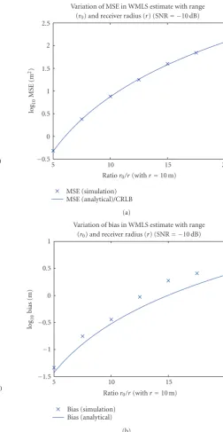
The performance of the WMLS algorithm as a function of range/baseline ratio (r0/r) is presented inFigure 2. For these
plots, the radius of the receiver array was fixed at 10 meters and the SNR was fixed at−10 dB. Once again, the simula-tion results are in good agreement with the analytical re-sults. At this relatively low SNR level, an MSE of approxi-mately 0.50 m2 and a total bias of approximately 0.04
me-ters are achievable with a range/baseline ratio of 5. For a range/baseline ratio of 20, the MSE increases to approxi-mately 125.9 m2and the total bias increases to approximately
2.24 meters. In this case (baseline fixed at 10 meters), this corresponds to a relative location error of approximately 0.71% for a range/baseline ratio of 5 and a relative location error of approximately 11.2% for a range/baseline ratio of 20. As indicated in (38), if the range/baseline ratio remains fixed, the relative location error decreases linearly as range increases; whereas, for a fixed baseline radius, the relative lo-cation error increases linearly with increasing range.
Performance as a function of number of receiver sensors
−1.5
−1
−0.5 0 0.5 1 1.5 2 2.5 3 3.5
log
10
MSE
(m
2)
−30 −25 −20 −15 −10 −5 0 5 10 SNR (dB)
MSE (simulation) MSE (analytical)/CRLB
Variation of MSE in WMLS estimate with SNR (r0=100 m,r=10 m)
(a)
−3
−2.5
−2
−1.5
−1
−0.5 0 0.5 1 1.5 2
log
10
bias
(m)
−30 −25 −20 −15 −10 −5 0 5 10 SNR (dB)
Bias (simulation) Bias (analytical)
Variation of bias in WMLS estimate with SNR (r0=100 m,r=10 m)
(b)
Figure1: WMLS MSE (a) and total bias (b) as a function of SNR.
Figure 3. For these plots, the radius of the receiver array was
fixed at 10 meters, the target range was fixed at 100 meters, and the SNR was fixed at−10 dB. The analytical results are again in good agreement with the simulated results with the exception of the caseM =4. For this case, the analytical ex-pression for the bias clearly understates the actual bias of the algorithm. This appears to result from the fact that some of the “negligible” terms dropped in the derivation of the ana-lytical expression for the bias are in fact not negligible when
M=4.
−0.5 0 0.5 1 1.5 2 2.5
log
10
MSE
(m
2)
5 10 15 20
Ratior0/r(withr=10 m) MSE (simulation)
MSE (analytical)/CRLB
Variation of MSE in WMLS estimate with range (r0) and receiver radius (r) (SNR= −10 dB)
(a)
−1.5
−1
−0.5 0 0.5 1
log
10
bias
(m)
5 10 15 20
Ratior0/r(withr=10 m) Bias (simulation)
Bias (analytical)
Variation of bias in WMLS estimate with range (r0) and receiver radius (r) (SNR= −10 dB)
(b)
Figure 2: WMLS MSE (a) and total bias (b) as a function of
range/baseline ratio.
AsFigure 3indicates, the achievable MSE with 4
receiv-ing sensor is approximately 19.95 m2and the achievable total
bias is approximately 0.20 meters. With 11 receiving sensors, the achievable MSE decreases to approximately 6.17 m2but
0.7 0.8 0.9 1 1.1 1.2 1.3 1.4
log
10
MSE
(m
2)
4 5 6 7 8 9 10 11
Number of sensors (M+ 1) MSE (simulation)
MSE (analytical)/CRLB
Variation of MSE in WMLS estimate with number of sensors (SNR= −10 dB,r0=100 m,r=10 m)
(a)
−4
−3.5
−3
−2.5
−2
−1.5
−1
−0.5 0
log
10
bias
(m)
4 5 6 7 8 9 10 11
Number of sensors (M+ 1) Bias (simulation)
Bias (analytical)
Variation of bias in WMLS estimate with number of sensors (SNR= −10 dB,r0=100 m,r=10 m)
(b)
Figure3: WMLS MSE (a) and total bias (b) as a function of number of receiving sensors.
Performance as a function of sensor position error variance
The performance of the WMLS algorithm as a function of the variance of random sensor position error is presented
inFigure 4. Again for these plots, the radius of the receiver
array was fixed at 10 meters, the target range was fixed at 100 meters, and the SNR was fixed at −10 dB. To reflect the fact that sensor errors will generally remain fixed over a large number of independent location estimates, the au-tocorrelation matrix and bias vector were estimated by av-eraging over a large number of independent trials for each set of randomly generated sensor errors before computing the MSE and total bias estimates that are plotted inFigure 4.
0.8 1 1.2 1.4 1.6 1.8 2 2.2 2.4 2.6
log
10
MSE
(m
2)
10−6 10−5 10−4 10−3 10−2
Variance of sensor position errorσ2
ε(m2)
MSE (simulation) MSE (analytical 1)
MSE (analytical 2) CRLB
Variation of MSE in WMLS estimate with errors in sensor position (SNR= −10 dB,r0=100 m,r=10 m)
(a)
−0.6
−0.4
−0.2 0 0.2 0.4 0.6 0.8 1 1.2
log
10
bias
(m)
10−6 10−5 10−4 10−3 10−2
Variance of sensor position errorσ2
ε(m2)
Bias (simulation) Bias (analytical 1) Bias (analytical 2)
Variation of bias in WMLS estimate with errors in sensor position (SNR= −10 dB,r0=100 m,r=10 m)
(b)
Figure4: WMLS MSE (a) and total bias (b) as a function of sensor position error variance.
In this case, the plots show two different “analytical” curves: Analytical 1 and Analytical 2. The curves labeled Analyti-cal 1 correspond to the MSE and bias predicted by (32), respectively, and these curves are in excellent agreement with the simulation results. The curves labeled Analytical 2, on the other hand, correspond to the MSE and bias pre-dicted by (32) under the assumption thatW1 = W. These
curves represent the performance of a “genie-aided” version of the WMLS algorithm in which the weighting matrixW1
is computed using the true values of the sensor position errors.
small in the low-sensor-noise regime where the dominant source of error is the TDOA measurement noise, but the bias (and consequently the MSE) increases dramatically as the sensor position errors become the dominant error mech-anism. Second, the increase in bias due to the presence of sensor position errors can be effectively eliminated from the WMLS by using the “correct” version of the weighting ma-trixW1in the algorithm. Although this is not actually
feasi-ble without modifying the algorithm extensively to estimate both sensor and target positions simultaneously, it does pro-vide some insight into how the algorithm fails when sensor position errors are present and indicates how critical it is to account for possible sensor position errors in UWB location estimation algorithms.
Finally, the behavior of the CRLB relative to the MSE of the WMLS algorithm is of interest. First, notice that the CRLB curve does not always fall below either the simulated MSE or the Analytical 1 MSE curve. This is probably a re-sult of the fact that the CRLB was derived assuming that the sensor position errors were i.i.d. zero-mean Gaussian that vary from estimate to estimate while the Analytical 1 curve and the simulated MSE were both computed by averaging over a relatively small number of random sensor position error vectors that were held fixed over a large number of independent location estimates. If the results had been av-eraged over a much larger number of random sensor er-rors (which would have required a much longer simulation time), both the Analytical 1 curve and the simulation results may well have fallen above the CRLB curve.7Notice also that
the bias of the WMLS estimate accounts for almost the en-tire MSE. Hence, while smoothing location estimates using a tracker will significantly reduce the CRLB, the bias of the WMLS will remain fixed and the MSE will remain corre-spondingly high. Finally, the fact that the CRLB, which cor-responds to purely random sensor position errors that can-not be accurately determined, is much larger than the Ana-lytical 2 MSE curve in the high-sensor-noise regime, which again indicates that it is essential to design UWB location es-timation algorithms that are able to adapt to and compensate for the systematic sensor position errors that often occur in practice.
4.2.2. Performance comparison of WMLS, WTLS, and N-R algorithms
In this subsection, we present simulation results compar-ing the performance of the WMLS algorithm with the new WTLS algorithm and the N-R algorithm. For these simu-lations, the baseline radius was fixed at 10 meters and the target range at 100 meters. Performance is compared both with and without the introduction of random sensor er-rors and both with and without averaging over multiple estimates.
7Recall, however, this is not a theoretical requirement since the CRLB is a lower bound only for the variance (and therefore the MSE) of unbiased estimates of location, while the WMLS has a significant bias.
One-shot estimation with no errors in sensor position
The performance of the three algorithms for one-shot lo-cation estimates with no errors in sensor position is pre-sented in Figure 5. For these results, the SNR was varied across a very wide range from −10 to 30 dB. As expected, the MSE of the WMLS algorithm is only slightly above the CRLB across the entire SNR range and approaches the CRLB asymptotically as the SNR becomes high. Further, as one might anticipate given the excellent MSE performance of the WMLS algorithm, the MSE for the (approximate maximum-likelihood) N-R algorithm is virtually identical to that of the WMLS algorithm, while the MSE of the WTLS algorithm is consistently (except for extremely low SNR) higher than both of the others. The degradation in MSE for the WTLS corre-sponds to a loss of approximately 1 dB in SNR across most of the SNR range.
Also as expected, the bias of both the WTLS and N-R al-gorithms is considerably lower than the bias of the WMLS algorithm for the entire range of SNR values. The reduc-tion in bias seems to correspond to an average gain of ap-proximately 5 dB in SNR across the SNR range. Note that for the WMLS algorithm, the bias dominates the MSE in the very low SNR regime but is negligible in the very high SNR regime so that the variance of the estimate dominates the MSE. For both the WTLS and N-R algorithms, the effect of the bias on the MSE is much less severe in the very low SNR regime.
Block averaging with no errors in sensor position
The performance of the three algorithms for smoothed es-timates computed by averaging over a block of 100 consec-utive one-shot estimates with no errors in sensor position is presented in Figure 6. As expected, the bias of the three algorithms has not changed as a result of the block averag-ing, but the MSE has decreased overall. These results demon-strate quite clearly the different manner in which the bias and variance of the one-shot location estimates affects the final smoothed estimate that would be produced by a tracker. In particular, in the very high SNR regime, where the error in the one-shot estimates is dominated by the variance of the estimates, the MSE of the averaged estimate is reduced by a factor of 100 for all three algorithms and approaches the CRLB. In contrast, the behavior in the very low SNR regime is quite different. In this case, the MSE of all three algo-rithms is far above the CRLB, but the MSE of the WMLS algorithm, which is dominated by the bias in this region, has not been reduced at all. On the other hand, the MSE of the WTLS and N-R algorithms, which are much closer to unbiased in this region, has been reduced by a factor of approximately 10.
One-shot estimation with errors in sensor position
The performance of the three algorithms for one-shot loca-tion estimates with errors in sensor posiloca-tion is presented in
−2
−1 0 1 2 3 4 5
log
10
MSE
(m
2)
−30 −25 −20 −15 −10 −5 0 5 10 SNR (dB)
MSE (WMLS) MSE (WTLS)
MSE (N-R) CRLB Comparison of MSE of algorithms
with SNR (r0=100 m,r=10 m)
(a)
−3
−2.5
−2
−1.5
−1
−0.5 0 0.5 1 1.5 2
log
10
bias
(m)
−30 −25 −20 −15 −10 −5 0 5 10 SNR (dB)
Bias (WMLS) Bias (WTLS)
Bias (N-R)
Bias (WMLS analytical) Comparison of bias of algorithms
with SNR (r0=100 m,r=10 m)
(b)
Figure5: Comparison of MSE (a) and total bias (b) for WMLS, WTLS, and N-R algorithms for one-shot estimation with no sensor errors.
the variance of the sensor position noise was varied from 10−6m2to 10−2m2. This range was chosen so that the error
in the one-shot location estimates is dominated by TDOA errors at the low end of the range of sensor position error variance but dominated by sensor position errors at the high end. Note however, that even at the high end of the range, the standard deviation of the sensor positions from the nominal position on a circle of radius 10 m is only 1 cm, which is still quite small.
These results demonstrate quite clearly the detrimental effects of even a small amount of sensor position error on
−4
−3
−2
−1 0 1 2 3 4
log
10
MSE
(m
2)
−30 −25 −20 −15 −10 −5 0 5 10 SNR (dB)
MSE (WMLS) MSE (WTLS)
MSE (N-R) CRLB Comparison of MSE of algorithms with SNR over 100 observations (r0=100 m,r=10 m)
(a)
−4
−3
−2
−1 0 1 2
log
10
bias
(m)
−30 −25 −20 −15 −10 −5 0 5 10 SNR (dB)
Bias (WMLS) Bias (WTLS)
Bias (N-R)
Bias (WMLS analytical) Comparison of bias of algorithms with SNR over 100 observations (r0=100 m,r=10 m)
(b)
Figure6: Comparison of MSE (a) and total bias (b) for WMLS, WTLS, and N-R algorithms for smoothed estimation with no sensor errors.
0.8 1 1.2 1.4 1.6 1.8 2 2.2 2.4 2.6
log
10
MSE
(m
2)
10−6 10−5 10−4 10−3 10−2
Variance of sensor position errorσ2
ε(m2)
MSE (WMLS) MSE (WTLS)
MSE (N-R) CRLB
Comparison of MSE of algorithms for one-shot estimation with errors in sensor position (SNR= −10 dB,r0=100 m,r=10 m)
(a)
−1
−0.5 0 0.5 1 1.5
log
10
bias
(m)
10−6 10−5 10−4 10−3 10−2
Variance of sensor position errorσ2
ε(m2)
Bias (WMLS) Bias (WTLS) Bias (N-R)
Comparison of bias of algorithms for one-shot estimation with errors in sensor position (SNR= −10 dB,r0=100 m,r=10 m)
(b)
Figure7: Comparison of MSE (a) and total bias (b) for WMLS, WTLS, and N-R algorithms for one-shot estimation with sensor er-rors.
Block averaging with errors in sensor position
The performance of the three algorithms for smoothed esti-mates computed by averaging over a block of 100 consecu-tive one-shot estimates with errors in sensor position is pre-sented inFigure 8. Again, as expected, the bias of the three algorithms has not changed as a result of the block aver-aging, but in this case, the MSE has decreased significantly only in the region where the errors in location estimation are dominated by TDOA errors. In the region above there is ap-proximately 1 mm of standard deviation in sensor position
−1.5
−1
−0.5 0 0.5 1 1.5 2 2.5
log
10
MSE
(m
2)
10−6 10−5 10−4 10−3 10−2
Variance of sensor position errorσ2
ε(m2)
MSE (WMLS) MSE (WTLS)
MSE (N-R) CRLB
Comparison of MSE of algorithms for smoothed estimation with errors in sensor position (SNR= −10 dB,r0=100 m,r=10 m)
(a)
−1.5
−1
−0.5 0 0.5 1 1.5
log
10
bias
(m)
10−6 10−5 10−4 10−3 10−2
Variance of sensor position errorσ2
ε(m2)
Bias (WMLS) Bias (WTLS) Bias (N-R)
Comparison of bias of algorithms for smoothed estimation with errors in sensor position (SNR= −10 dB,r0=100 m,r=10 m)
(b)
Figure8: Comparison of MSE (a) and total bias (b) for WMLS, WTLS, and N-R algorithms for smoothed estimation with sensor errors.