1
A Comparative Analysis of On-line
Measurement-based Capacity Allocation Schemes
Fatih Hacı¨omero˘glu
∗and Michael Devetsikiotis
†Department of Electrical and Computer Engineering
North Carolina State University
Raleigh, NC 27606-7911, USA
†
[email protected]
∗
[email protected]
Submitted to ITC 18, Berlin, August 2003
Abstract— Today’s high-speed packet-switched net-works are faced with the task of handling an increasing amount and variety of services, requiring different QoS constraints. Within the context of such traffic demands the choice of appropriately accurate but also practically
implementable measurement algorithms becomes crucial.
In this paper, we perform a comparative study of alternative on-line bandwidth allocation algorithms, we analyze their complexity, and perform comparisons via simulation experiments. Our motivation is to use these algorithms in the data plane of “self-sizing” frameworks, and make use of their output in taking control plane decisions either locally or globally, in an on-line fashion. Previously, no such comprehensive comparison of relevant methods has been carried out, especially from a combined accuracy versus implementation complexity point of view. Due to the dynamic characteristics of the algorithms, we encounter the choice of time resolution, i.e., measurement time scale and window. After numerous simulations, we gain insight on the critical effect of these choices on the performance of the algorithms. We deduce that the time scale parameter itself can be determined dynamically so that measurement-based algorithms perform successfully independent from the varying traffic conditions. Finally, we demonstrate the effectiveness of this new approach over the static one.
I. MOTIVATION ANDINTRODUCTION
The demand on high-speed networks is getting higher and tougher to satisfy everyday, with the invention and commercialization of new bandwidth-hungry applications. Network resources are to be increased accordingly, to sustain an acceptable level of service. However, it is not always feasible to
increase resources at the same pace of the increase in the traffic demand. In this regard, the bandwidth allocation in high-speed QoS-oriented networks is critical and needs to be made dynamic, adaptive and measurement-based, rather than static, to attain a more efficient use of resources. Especially for net-work links shared through statistical multiplexing, adaptive bandwidth allocation algorithms based on traffic measurements can achieve important gains.
For these reasons, we performed a comparison of on-line, dynamic measurement-based bandwidth allocation algorithms, which have low time com-plexity, and are based only on measurements instead of unreasonable assumptions about the incoming traffic. To the best of our knowledge, no such com-prehensive comparison of relevant methods has been previously carried out, especially from a combined accuracy versus implementation complexity point of view.
traf-fic class or “band”. Periodically, the output of the al-gorithms, which give the required capacity demands of the traffic types, are collected, and either locally or globally, a control plane action is taken (i.e., the virtual links or scheduling allocations are re-calculated) so as to minimize a predefined objective such as bandwidth cost or maximize revenue.
In this context, it is very important to choose mea-surement methods that satisfy stringent constraints in terms of both accuracy and complexity. Most of the algorithms we used in this paper naturally orig-inated from the effective bandwidth concept, since effective bandwidth is the amount of the required bandwidth to be allocated for the satisfaction of a QoS constraint. Furthermore, in the literature, we identified two research areas which are related to our aim. These are network traffic prediction [3]–[6] and measurement-based admission control (MBAC) [7]–[9].
MBAC algorithms are composed of separate mea-surement procedure and admission criterion. We investigated the applicability of these separable measurement procedures for our purposes. However, other than the trivial Gaussian Approximation band-width estimator, such methods are not suitable for on-line re-sizing due to the fact that either they rely on unreasonable information (i.e., they presume that a priori traffic descriptors, such as present number of connections are known) or they have unacceptable computational complexity.
These incompatibilities stem from the different design considerations between measurement-based estimators in MBAC and self-sizing frameworks. First, MBACs are designed to operate only in the ingress nodes, where admission decisions are
taken. Second, the period of execution of MBAC
algorithms is at the connection level time scales. Our aim is to obtain on-line algorithms, working
on every node in the network. Therefore their
timescale and computational complexity are smaller than connection level timescales. Similar to MBAC
algorithms, traffic predictors do not suit our consid-eration either. The reason this time is not because
they are centralized and computationally complex as in MBAC algorithms, but that they do not target
a QoS constraint.
The algorithms in this paper take a window of
traffic measurements as input, estimate the parame-ters they need in a bandwidth allocation calculation
formula and output the required amount of capacity
to be reallocated. The measurements correspond to the amount of incoming traffic during a slot
duration,tslot. Consequently, the algorithm is called
periodically everyN∗tslot seconds (the reallocation
period), whereN is the window size. The choices of
tslot and N are critical [10] and affect significantly
the performance of algorithms.
In our simulations, the performance metric is
related to a QoS constraint, in our case packet loss
probability. To quantify the amount of expanded resources, we use two cost metrics, namely,
• Allocation Ratio (Average Capacity
Alloca-tion divided by Average Traffic Rate)
• Average Queue Occupancy
Our purpose is to obtain a feasible algorithm
which is able to use bandwidth optimally (i.e., dynamically as in Figure 2) while still obtaining
a performance close to the QoS target. The ideal
unreasonable assumptions on the traffic, and be based completely on measurements.
The remainder of the paper is structured as fol-lows. After describing the algorithms in Section II, we compare their response to different scenarios (i.e., variable buffer size, level of aggregation of sources, long-range dependence of traffic,
compu-tational and memory complexity requirements) and choose promising ones for further simulation study in Section III. Then we explain our simulation methodology in Section IV. Later, simulation re-sults highlighting the importance of measurement time scales in algorithm performance are presented in section V. Section VI introduces the use of a
measurement-based time scale and shows its
effec-tiveness over the static time scale approach. Finally, we conclude with a discussion of the results and outline prospects for further enhancements.
II. ALGORITHMS
A. Direct EB Allocation (DEB)
DEB algorithm relies on a direct analytical eval-uation, using the definition in [11].
eb(s, t) = ln(E(e
sX(0,t)))
st (1)
X(0, t) is the amount of incoming work during a duration oft. The (s, t)parameters are the so-called space and time parameters. Parametersis calculated by using Large Deviations Theory (LDT) and by making a large buffer assumption. The overflow probability is calculated from an asymptotically
exponential decrease assumption.
P(B < Q) = e−s(C)B (2)
The time parameter t is related to time scales which are responsible for buffer overflow. It should be chosen small enough so that traffic is observed for buffer overflow analysis. Finally, the expecta-tion in (1) is approximated by a time average, as suggested in [12].
The empirical evaluation of (1) is simulated and compared with analytical effective bandwidth of known Poisson and ON-OFF source types in [13].
B. Courcoubetis EB Allocation (CEB)
This method [14] is based on LDT and a large buffer assumption, similar to the DEB algorithm:
eb =m+ IDs
2B (3)
The parameters m, B, s and ID are the mean rate, buffer size, space parameter and index of dispersion of X[0, t]. The space parameter s is calculated using (2).
ID estimation process has a computational com-plexity proportional to N2.
ID =Var(X(0, t)) (4)
1 + 2
1/4N
X
k=1
1−4k−1
N
!
AC(k)
N
X
k=1
X(0, t)
N
!−1
C. Many Sources Asymptotic EB Allocation (MSAEB)
made, instead of a Large Buffer assumption, while using LDT to solve the problem of estimation of the space and time parameters (s, t). As described in [15], ifM sources are multiplexed in bufferB, rj
is the percentage of streams of typej, and maximum allowed buffer overflow probability to be guaranteed is e−a, then minimum required bandwidth can be
calculated by solving
C = sup
s (infs (R(s, t))) (5)
where
R(s, t) = stM
P
jrjeb(s, t) +a
st −
B
t (6)
In (6), eb(s, t) term is found from (1).
For a givent, theR(s, t)is a unimodal function of
s, having a unique minimizer. Then,R(s, t) =Rt(s)
is solved by using a golden section search method as described in [15]. This process is repeated for a range of t values smaller than the measurement window time, and the maximum among them is taken as the required capacity to be allocated.
D. ON-OFF EB Allocation (OOEB)
The idea is to obtain estimation values of an equivalent ON-OFF traffic model from measure-ments, and substitute them in the specific analyt-ical effective bandwidth formula (7) for ON-OFF sources [16].
eb(s, t) = −sr+a+b−1/2 (−sr+a−b)
2−
2ba
2s
(7) Parameters a, b and r denote a ON-OFF traffic model where ON and OFF periods are exponentially distributed with parameters a and b respectively,
and r is the constant traffic generation rate in the
ON state. These parameters can be estimated by
matching the first three moments of N data
mea-surements falling into the window. These
estima-tions have difficulties and require search algorithms,
since direct solution of high order equations is not
trivial. Moreover, this method is weak because of
the limited fitting spectrum of ON-OFF model [17].
E. Norros EB Allocation (NEB)
In [18], besides introducing modeling of real
traffic by fractional Brownian motion (FBM), an
effective bandwidth formula (8) for FBM is also
given.
eb =m+ (8)
K(H)q−2 ln(Ploss)
H ∗
a
2H ∗B −
1−H
H ∗
m
2H
where K(H) = HH(1−H)1−H
and m, H, P loss,
x and a are the mean, Hurst parameter, buffer
overflow probability, buffer size and coefficient of
variation respectively. Parametera, is approximated
by the index of dispersion. In fact, this is a valid
assumption only when the traffic is short range
dependent.
The Hurst parameter can be set from a priori
mea-surements. However, to react to unexpected traffic
changes, a measurement-based on-line algorithm is
favored. Difficulties of H estimation methods are
analyzed in [19], where the comparison of several
H estimation algorithms revealed that Abry-Veitch
estimator (AV estimator) based on Wavelet theory
F. DRDMW (Improved Empirical EB Allocation)
This method in [21] is an improved version of empirical effective bandwidth methods. A unified phenomenological framework to estimate overflow
probability of both long range dependence (LRD) and short-range dependence (SRD) is put forward by including the Hurst parameter in traditional an-alytical effective bandwidth methods.
P(B < Q) =e−s(C)B2−2H (9)
Second, the difficulty of measuring the effective bandwidth of real-time traffic online by using direct
estimator [21] is alleviated by using an approach based on dual recursive algorithm with double mov-ing windows (DRDMW), which is introduced in an empirical calculation of analytical effective band-width formula instead of using the direct estimator.
G. Gaussian Approximation Allocation (GA)
The simplest resource allocation method existing
in literature is the GA method [22], where link buffer is ignored and server capacity is set according to Gaussian arrival rate distribution:
C =m+σ∗q−2∗ln (Ploss)−ln (2∗π) (10)
wherem andσare the mean and standard deviation of the arrival rate distribution.
III. COMPARISON OF THEALGORITHMS
The first algorithm, namely Direct Effective Bandwidth Allocation algorithm, relies on the effec-tive bandwidth formula, and possesses the problem
of finding appropriate values for s and t, which
depend on QoS requirements and the system pa-rameters. The space parameter is estimated using the Large Buffer Assumption. The time parameter estimation is left somewhat arbitrary, for the time being.
The second algorithm uses (3, which is an al-ternative generic effective bandwidth definition in terms of the mean rate, index of dispersion, QoS parameter and buffer size. It is simpler, but it still doesn’t address long range dependent traffic.
The Many Sources Asymptotic Effective Band-width algorithm relies on the effective bandBand-width formula (1) and encounters the problem of estima-tion of (s, t). This method accomplishes it by solv-ing a functional optimization problem. Although it is a very innovative approach, this may be too slow for our motivational self-sizing scenario where every node takes on-line measurements of every traffic type.
The ON-OFF Effective Bandwidth formula (7) for our fourth method is obtained by substituting an ON-OFF arrival process instead of X(0, t) in the analytical effective formula. With regard to a practical usage of such expressions, we encountered other problems than estimation of (s, t)parameters, such as model parameter estimation, and goodness of fit of the model.
is not valid for traffic formed by small number of sources. This places a constraint on the source type, however our aim is to have an algorithm capable of functioning without unreasonable assumptions.
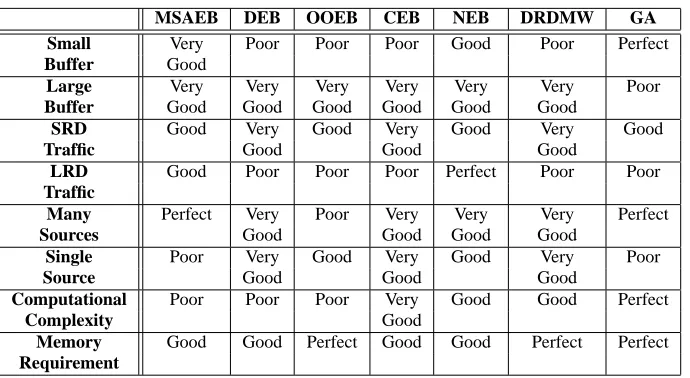
The self-similarity is addressed only in the NEB and in the DRDMW method. Others do not dis-criminate between short range dependence and long range dependence. Although the index of dispersion in the Courcoubetis formula of the second algorithm stands for burstiness of the source, the formula is not for long range dependent traffic. Thus the effective bandwidth approximation on which Courcoubetis formula is based, (i.e., exponential decay of buffer overflow probability with increasing buffer size) is not valid for self-similar traffic (the decay is hy-perbolic and slower than exponential). We provide a summary of our performance comparisons with respect to various network scenarios in Table I.
The Gaussian Approximation algorithm is the easiest to implement, and suitable to be used as an algorithm setting an upper bound, since it does not consider buffer size. The Courcoubetis Effective Bandwidth Allocation is also another easy, and promising one, since this one takes into account buffer also. But neither of the previous two algo-rithms is designed with long range dependent traffic in mind. Norros effective bandwidth and DRDWM algorithms are the only ones incorporating the Hurst parameter, therefore addressing to long range dependent traffic. Although DRDMW is designed to alleviate the numerical overflows in the direct effective bandwidth allocation, that problem can not be completely alleviated due to the structure of (1). Therefore, we picked the following three algorithms for further simulation analysis:
• Gaussian Approximation (GA)
• Courcoubetis Effective Bandwidth Allocation
(CEB)
• Norros Effective Bandwidth Allocation (NEB)
IV. SIMULATIONMETHODOLOGY
The selected on-line measurement-based resource allocation algorithms are implemented and tested in a simulation scenario as shown in Figure 1. This is
a single server queue simulation where the service rate is changed, in an on-line fashion, periodically based on recent traffic measurements. We used the
Sup-FRP traffic model [23]. The simulation flow slides packet by packet, emulating a real case sce-nario as in an Ethernet card passing packets to upper network layers.
. . .
tslot
[ X1, X2, ... , XN ] Number of Arrivals
time
Buffer
Dimensioning Algorithm
C
Fig. 1. Simulation scenario.
Figure 2 gives a visual representation of how algorithms adjust service rates, tracking fluctuations in the incoming traffic rates, so as not to waste
resources.
We performed simulations with 5 different tslot
values (0.01, 0.05, 0.1, 0.5, 1s) and 5 window sizes
(N) values (3, 6, 30, 60, 300slots) in every method. Therefore, we had 25 simulations per method. As a total, we present here results of 75 simulations.
TABLE I
PERFORMANCECOMPARISONS
MSAEB DEB OOEB CEB NEB DRDMW GA Small Very Poor Poor Poor Good Poor Perfect
Buffer Good
Large Very Very Very Very Very Very Poor
Buffer Good Good Good Good Good Good
SRD Good Very Good Very Good Very Good
Traffic Good Good Good
LRD Good Poor Poor Poor Perfect Poor Poor
Traffic
Many Perfect Very Poor Very Very Very Perfect
Sources Good Good Good Good
Single Poor Very Good Very Good Very Poor
Source Good Good Good
Computational Poor Poor Poor Very Good Good Perfect
Complexity Good
Memory Good Good Perfect Good Good Perfect Perfect
Requirement
Fig. 2. A visual example view of dynamic capacity allocation.
resulted after 30 simulation replications and confi-dence intervals are insignificant.
In all of the simulations in this section, we generated traffic with the same mean value of 20 Kbytes/s, the same Hurst parameter of 0.7 and the same buffer size of 5 Kbytes. We set the QoS target to packet loss probability of 10−3, so as to have a
common ground for the performance comparisons
of algorithms in the simulation scenario (Figure 1). Note that the average traffic rate of 20 Kbytes/s is the product of an average packet size of 200 bytes and average packet arrival rate of 100 packets/s. Therefore, the average time between two consec-utive packets is 0.01 seconds and the tslot values
chosen in the simulations, which are (0.01, 0.05, 0.1, 0.5, 1s), correspond to cases where 1, 5, 10, 50 and 100 packet arrivals take place on average in a slot time duration, respectively. Also note that the choices fortslotandN are made deliberately to have
simulations where reallocation takes place in every 3 seconds, but with different measurement resolution in the recent history of the measurement data. For example, a simulation with (0.01s, 300slots) includes 300 measurements, whereas the one with (1s, 3 slots) includes three measurements in the same recent 3 seconds history.
The combined, on-line Hurst parameter and EB estimation is beyond the scope of this paper and
is left as future work.
V. SIMULATIONRESULTS
In this section, we first present performance and cost plots. We demonstrate and observe the impor-tance of time scale choice in measurement-based algorithms.
The plots in this section are in the form of three dimensional graphs. The xy plane is composed of slot duration and window size pair, i.e., (tslot, N).
There are 25 z coordinate points coming from the
convolution of 5 values of tslot and 5 values of
N, which are (0.01, 0.05, 0.1, 0.5, 1s) and (3, 6, 30, 60, 300slots), respectively. We chose to present simulation results in this form, rather than listing the numbers in a table form, because it would be difficult in the table form to observe the trends of
the data when the time slot length increases while the window size is kept constant and vice a versa. At the end of this section, we provide the processing time plots with respect to the window sizes.
A. Performance Plots
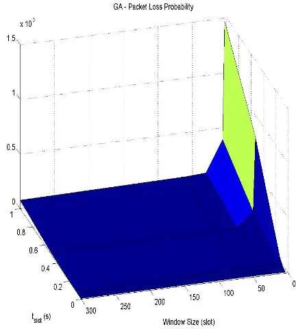
The following three plots show the performance results for different tslot and N values in the
sim-ulation scenario given in Figure 1. Figure 3 shows the loss probability results when GA is used for link dimensioning.
As seen from Figure 3, the loss probability in-creases when tslot is increased while N is kept
constant. Furthermore, it can be deduced that the loss probability decreases when N is increased
while tslot is kept constant.
Fig. 3. Loss probability against different time slot length and window size values, when GA is used for dynamic resource allocation.
The QoS target, which is 10−3, is satisfied in every (tslot, N) combination with the exception of
(tslot = 1s, N = 3slots). Note that GA is used as
an upper band of resource allocation for comparison
purposes. It does not consider buffer size. In fact, it assumes there is no buffer. This is why, it is expected to be more generous than other algorithms. The fact that a violation of QoS took place in this
method implies trouble for other methods.
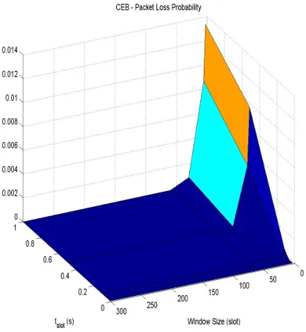
Figure 4 tells us that the CEB’s performance changes similar to GA againsttslotandN variations,
but Ploss values are relatively about an order of
magnitude higher. The QoS target is violated for the following (tslot, N)pairs: (0.5s, 3slots), (1s, 3slots),
(0.5s, 6slots) and (1s, 6slots). This algorithm,
con-sidering the presence of buffer, theoretically permits lesser resource usage than GA.
The loss probability results of NEB are provided
Fig. 4. Loss probability against different time slot length and window size values, when CEB is used for dynamic resource allocation.
Fig. 5. Loss probability against different time slot length and window size values, when NEB is used for dynamic resource allocation.
are between the ones of GA and CEB. However, whenN is either 30, 60 or 300,Ploss is smaller than
other algorithms, which implies an over-allocation of bandwidth.
B. Cost Function Plots
The plots in this section show how much
re-sources are used while getting the performance
results introduced in the previous section.
The following two plots are cost plots for GA.
Figure 6 agrees with Figure 3 and shows that as
tslot is increased for a constant N, the allocation
ratio decreases towards 1. We also observe that for
constanttslot, increasingN results in a larger
capac-ity allocation. But this rate of increase in capaccapac-ity
allocation depends on the tslot value. For instance,
whentslot length is fixed to 1s, the allocation ratios
for N =3, 6, 30, 60 and 300 are 1.34, 1.40, 1.46,
1.47 and 1.51, respectively. However, when tslot is
set to 0.01s, the corresponding ratio values are 4.21,
5.02, 5.89, 6.23 and 9.28. So, once tslot is properly
chosen, choosingN looses its importance, since the
change in the ratio values are much smaller.
Figure 7 is in accordance with Figure 6 and Figure 3, and gives an idea about how much buffer is occupied. Figures 3, 7 and 6 show the importance of time scale choice. We observe that even if GA does not consider buffer, it can still be an acceptably good resource allocator, given that tslot and N values are
chosen properly.
Fig. 7. Average Queue Occupancy against different time slot length and window size values, when GA is used for dynamic resource allocation algorithm.
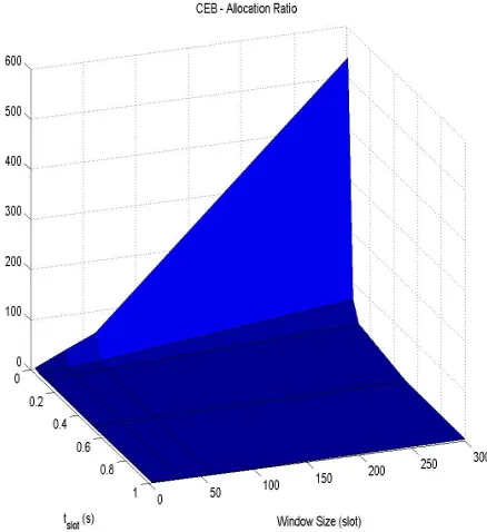
Figures 8 and 9 are cost plots when CEB is used as the dynamic resource allocation method. Figure 9 shows that the buffer occupancy changes drastically with the choice of N. For small N, the occupancy is bigger than the one for GA, but for big window size values (60 and 300), the buffer is less occupied than when GA is used as resource allocator. These implications are justified in Figure 8. As a result, this shows that if N is chosen poorly, the resource allocation can be even worse than GA’s allocation.
Compared to GA, we observe that bigger tslot
values lead to better allocation ratios (i.e., ratios
Fig. 8. Ratio of the average capacity allocation to the average traffic rate against different time slot length and window size values, when CEB is used for dynamic resource allocation.
closer to 1) and the choice ofN has a greater effect
on CEB. With proper choice oftslotandN, the same
performance can be achieved with lesser resource
usage. To illustrate, when tslot is fixed to 1s, the
allocation ratios for N 3, 6, 30, 60 and 300 are
1.04, 1.08, 1.29, 1.54 and 3.88 respectively, and
when tslot is set to 0.01s, the corresponding ratio
values are 4.86, 8.45, 30.66, 58.25 and 540.13. Here,
similar to GA, we see the importance of choosing
tslotproperly. But unlike for GA, here choosingN is
also important. This is because the rate of increase
of ratio values when N is increased is much more
significant. Choosing a large N leads to serious
over-allocation. Also note that in the above cases
where allocation ratios are 1.04 and 1.08, the Ploss
values are 0.0134 and 0.0087 respectively, and the
QoS criterion of 10−3 is not satisfied by one order
Fig. 9. Average Queue Occupancy against different time slot length and window size values, when the CEB is used for dynamic resource allocation.
Figures 10 and 11 are cost metrics plots when NEB is used as the dynamic resource allocation method. Figure 10 shows that there exists over-allocation of resources when the window size is 30, 60 and 300, similar to the behavior observed in CEB.
When it comes to the choice of tslot, as in the
previous methods, a bigger tslot resulted in better
resource allocation. This method is the only one which allocates more capacity to the traffic possess-ing higher long-range dependence. Overall, it can be said that NEB includes similar performance and cost changes as the ones of CEB, but performance values are around one order of magnitude better, and consequently, cost values are higher. For example, for tslot and N pairs of (1s, 3slots) and (1s, 6slots),
the Ploss and allocation ratio values were 0.0134,
0.0087 and 1.04, 1.08, respectively, for CEB, but the corresponding values for NEB are 0.0022, 0.0003
Fig. 10. Ratio of the average capacity allocation to the average traffic rate against different time slot length and window size values, when NEB is used for dynamic resource allocation.
and 1.38, 1.61 respectively. This shows that NEB has a tendency of allocating more resources than CEB, and results in better QoS constraint satisfac-tion.
C. Complexity
Figure 12 shows the processing times of the algorithms as a function of window size values. The processing time is the time required for the algorithm to re-calculate capacity. The processing time is seen to be related to N for CEB and NEB, with a complexity of O(N2). This result is in parallel with our expectations. CEB and NEB calculate autocorrelations of measurements falling into the measurement window of size N, and this requires a processing time proportional to N2.
Fig. 11. Average Queue Occupancy against different time slot length and window size values, when NEB is used for dynamic resource allocation.
regardless of N, its execution time remains much
smaller compared to other algorithms.
Fig. 12. Processing times of algorithms vs. window size.
VI. DYNAMIC VS. STATICTIME SCALE
Sections V-A and V-B show how drastically the performances of the measurement-based capacity allocation algorithms change depending on the time scale choice.
Mainly, we observed that increasing the mea-surement slot, tslot, results in a decrease in the
capacity allocation and consequently an increase in
Ploss in all of the algorithms. This can be explained
intuitively from the structure of the formulas used in the capacity allocation algorithms. To illustrate, consider the Gaussian Approximation Algorithm’s formula (10), where m and σ are the mean and standard deviation of the most recent N measure-ments, [X1, X2, ..., XN]. EachXi represents
incom-ing traffic load in consecutive tslot durations. By
the law of large numbers, as tslot increases, say
tslot → A, where A is a time parameter, which is
large (dependent on the traffic characteristic), then
Xi approaches m ∗A for all i. This causes σ in
(10) to go to zero, and the capacity value, eb to approach to the mean rate, m. A similar reasoning can be given for other methods, in which not only standard deviation, but also autocorrelations of measurements, [X1, X2, ..., XN] are used.
On the other hand, we also observe that taking
tslot arbitrarily small ends up in over-allocation
of resources. As tslot decreases, the measurement
history (tslot ∗ N) decreases too. This decreases
the confidence and increases the randomness in the formula parameter estimations, yielding over-allocations.
We could obtain empirical tslot values from the
However this particular tslot value would be useful
only for the traffic that we used in our simulations. Consider using a traffic whose mean is m∗K (that is K times bigger). This time, on average K times more traffic load will fall on average into the slots. Relatively, this is the same experiment as using
K times bigger tslot measurement slots, with mean
traffic rate m. In other words, the measurement time scale is relative to the traffic characteristics. A static tslot may correspond to cases where we
described previously as small or large, depending on the incoming traffic.
As a result, we believe that the measurement time scale tslot should also change dynamically based on
measurements[X1, X2, ..., XN], in order to keep the
algorithms always working close to their best. In [25], the Maximum Time-Scale (MaxTS = t∗) is used as the time scale of interest for queueing systems feed by a fractal Brownian motion (fBm) process:
t∗ = kσH (C−m)
1 1−H
(11)
where k = q−2∗ln (Ploss), m is the mean traffic
rate, σ is the standard deviation of the traffic rate and C is the capacity of the server.
The value oft∗ is derived from (12), whereAˆH(t)
is the probabilistic envelope process of the fBm cumulative arrival processAH(t) (AH(0) = 0), such
that P(AH(t)>AˆH(t))≈Ploss:
dAˆH(t∗)
dt =C (12)
On the basis of the law of large numbers, as
t → ∞, dAˆH(t)
dt converges to the mean arrival rate.
ˆ
AH(t)increases with a decreasing rate aftert∗. This
means that the probability that the average arrival rate exceeds the link capacity decreases for t > t∗.
In the remaining of the paper, we test using a
dy-namic time scale by estimatingt∗using the recentN
measurements and taking tslot=t∗ as the
measure-ment slot duration for the next N measurements. In other words, besides effective capacity, tslot is also
recalculated after every N measurements.
Instead of the (C −m) term in (11), we used
L ∗ m, where L is taken as a constant L = (AllocationRatio)−1. The reason is that we al-locate capacity dynamically and do not have a constant C 1.Table II shows the improvement of using a dynamictslot=t∗ against statictslotchoices
(GA is used as the capacity allocation algorithm, and the Ploss target is set to10−3 as in the previous
simulations). As the mean rate increases, the per-formance of the static tslot cases changes (the ratio
decreases and Ploss increases), whereas the
perfor-mance of the dynamic tslot = t∗ case remains the
same. This shows that on-line measurement-based algorithms with constant measurement intervals are heavily dependent on the incoming traffic’s mean rate, whereas the ones with dynamic measurement intervals are more robust 2.
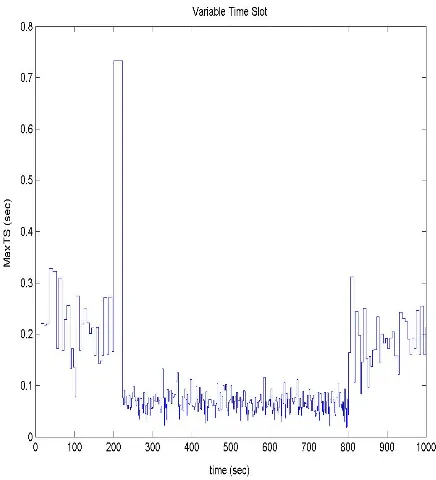
To illustrate the benefits visually, we generated a traffic trace of 1000s, where the mean rate of traffic between 200 and 800s is 5 times the mean rate at the remaining intervals. Figure 13 shows the dynamic capacity allocations. Note that the allocation ratios in the static tslot cases change in the region of
traffic with high mean rate. But the allocation ratio
1
We tried using the average capacity allocation instead ofC, but this caused a multiplicative effect, such that, when capacity allocation increases,C−mterm in (11) decreases. But decreasingtslotresults
in increased capacity allocation measurement in the next window, and this loop ends up havingt∗≈0.
2
The particular performance figures for dynamic tslot case in
Table II are dependent on the value of L (we used L = 1.5).
TABLE II
PERFORMANCEMETRICS VS. TIMESCALE
Mean tslot tslot tslot tslot
(Kbytes/s) 0.08s 0.4s 2s t∗
4 Ratio 4.751 2.657 1.745 1.915
Ploss 0 0 0.000003 0.000391
20 Ratio 2.952 1.739 1.353 1.914
Ploss 0 0.000009 0.000382 0.000696
100 Ratio 1.742 1.334 1.183 1.913
Ploss 0.000010 0.000332 0.002649 0.000910
remains roughly the same in the dynamic time scale case. This is achieved by adjusting tslotas shown in
Figure 15.
Fig. 13. Capacity allocations vs. traffic mean rate.
The number of packets dropped increases when the mean is increased gradually in Figure 14 (for
tslot = 0.01s, no loss occurred, due to
over-allocation). The t∗ case performs again in between
the static tslot cases. But note that when tslot =t∗,
the algorithm can self-adjust and perform similarly
against traffic mean changes, whereas the perfor-mance of an algorithm with static tslot is dependent
on the traffic. To illustrate, a method with static
tslot = 0.01s case will over-allocate significantly
when the mean rate decreases much below of 4Kbytes/s, and a method with static tslot = 2s
case will suffer significant degradation of the QoS target when the mean rate increases much above 100 Kbytes/s.
Fig. 14. Cumulative Number of Dropped Packets.
VII. SUMMARY ANDCONCLUSIONS
In this paper, we presented and compared measurement-based on-line capacity allocation al-gorithms and proposed a way to improve their robustness.
Fig. 15. The Plot of Dynamic Time Scale Parametert∗.
the measurements in the measurement window de-crease and the allocated capacity approaches the mean traffic rate. This causes the loss probability to increase.
Since the measurement time scale is directly related to the measured traffic, the result of a measurement-based algorithm using constant time scale is open to the performance degradations due to the changes in traffic trends. However, our aim was to obtain an algorithm which does not require any
a priori traffic knowledge, and which is based fully
on the measurements. Therefore we incorporated the Maximum Time-Scale (MaxTS) parameter and tested successfully adapting the measurement time scales based on measurements themselves.
To sum up, in this paper, we
• identified on-line measurement-based capacity
allocation algorithms,
• compared their performances analytically, • simulated promising ones,
• observed significant affects of the choice of
measurement time scale,
• proposed to vary measurement time scale
adap-tively,
• through an example, showed the performance
robustness of measurement-based algorithms, in which measurement time scale is adaptive (measurement-based).
The outcomes of this study can be used for choos-ing algorithms to be implemented in real switches, taking into account trade-offs of complexity, accu-racy and robustness.
ACKNOWLEDGMENTS
This research was partly supported by the Center for Advanced Computing and Communication -North Carolina State University, and by Alcatel. The authors thank Aziz Mohammed and Chao Kan of
Alcatel, Plano, for their comments and assistance.
REFERENCES
[1] Q. Hao, S. Tartarelli, and M. Devetsikiotis, “Self-sizing and optimization of high-speed multiservice networks,” in Proc. of
IEEE Globecom ’00, vol. 3, San Francisco, November 2000,
pp. 1818–1823.
[2] J. Yang and M. Devetsikiotis, “On-line estimation, network design and performance analysis with effective bandwidths,” in
Proc. of 17th ITC, Salvador Da Bahia, Brazil, December 2001.
[3] D. Morato, J. Aracil, L. A. Diez, M. Izal, and E. Magana, “On linear prediction of internet traffic for packet and burst switch-ing networks,” in Proc. of ICCCN ’01, Scottsdale, Arizona, October 2001, pp. 138–143.
[4] S. Ostring, H. Sirisena, and I. Hudson, “Rate control of elastic connections competing with long-range dependent network traffic,” IEEE Transactions on Communications, vol. 49, no. 6, pp. 1092–1101, June 2001.
[5] C. Huang, I. Lambadaris, M. Devetsikiotis, P.W.Gylnn, and A. Kaye, “DTMW; a new congestion control scheme for long-range dependent traffic,” in Proc. of 15th ITC, Washington, D.C., June 1997.
[6] M. Grossglauser, S. Keshav, and D. N. C. Tse, “RCBR: A simple and efficient service for multiple time-scale traffic,”
IEEE/ACM Transactions on Networking, vol. 5, no. 6, pp. 741–
755, 1997.
[8] P. Droz, “Wavelet-based resource allocation in atm networks,” in Proc. of IEEE Globecom ’97, vol. 2, Phoenix, Arizona, November 1997, pp. 833–837.
[9] J. Qiu and E. W. Knightly, “Measurement-based admission con-trol with aggregate traffic envelopes,” IEEE/ACM Transactions
on Networking, vol. 9, no. 2, pp. 199–210, 2001.
[10] M. Grossglauser and D. N. C. Tse, “A framework for robust measurement-based admission control,” IEEE/ACM
Transac-tions on Networking, vol. 7, no. 3, pp. 293–309, 1999.
[11] F. Kelly, Stochastic Networks: Theory and Applications. Ox-ford University Press, 1996, pp. 141–168.
[12] G. Kesidis, J. Walrand, and C. S. Chang, “Effective bandwidths for multiclass markov fluids and other atm sources,” IEEE/ACM
Transactions on Networking, vol. 1, no. 4, pp. 424–428, August
1993.
[13] S. Tartarelli, M. Falkner, M. Devetsikiotis, I. Lambadaris, and S. Giordano, “Empirical effective bandwidths,” in Proc. of IEEE
Globecom ’00, San Francisco, November 2000.
[14] C. Courcoubetis and R. Weber, “Buffer overflow asymptotics for a buffer handling many traffic sources,” Journal of Applied
Probability, vol. 33, pp. 886–903, 1996.
[15] C. Courcoubetis, V. A. Siris, and G. Stamoulis, “Application of the many sources asymptotic and effective bandwidths to traffic engineering,” Telecommunication Systems, vol. 12, no. 2-3, pp. 167–191, 1999.
[16] R. Gibbens and P. Hunt, “Effective bandwidths for the multi-type uas channel,” Queueing Systems, vol. 9, pp. 17–28, 1991. [17] S. Li, S. Park, and D. Arifler, “SMAQ: A measurement-based tool for traffic modeling and queueing analysis, part I - design methodologies and software architecture,” IEEE
Communica-tions, vol. 36, pp. 56–65, August 1998.
[18] I. Norros, “On the use of fractional brownian motion in the theory of connectionless networks,” IEEE Journal of Selected
Areas in Communications, vol. 13, no. 6, pp. 953–962, 1995.
[19] S. Molnar and T. D. Dang, “Pitfalls in long range dependence testing and estimation,” in Proc. of IEEE Globecom ’00, San Francisco, November 2000.
[20] D. Veitch and P. Abry, “A wavelet based joint estimator of the parameters of long-range dependence,” IEEE Transactions on
Information Theory, vol. 45, no. 3, pp. 878–897, 1999.
[21] W. Shen, “On-line measurement of effective bandwidth and a hierarchical self-sizing framework,” Master’s thesis, Institute for Electrical and Computer Engineering, Carleton University, April 2002.
[22] R. Guerin, H. Ahmadi, and M. Naghshineh, “Equivalent capac-ity and its application to bandwidth allocation in high-speed networks,” IEEE Journal of Selected Areas in Communications, vol. 7, no. 7, pp. 968–981, 1991.
[23] B. K. Ryu and S. B. Lowen, “Point process approaches to the modeling and analysis of self-similar traffic, I. model construc-tion,” in Proc. of IEEE Infocom ’96, vol. 3, San Francisco, March 1996, pp. 1468–1475.
[24] M. Roughan, D. Veitch, and P. Abry, “Real-time estimation of the parameters of long-range dependence,” IEEE/ACM
Trans-actions on Networking, vol. 8, no. 4, pp. 467–478, 2000.